Condensation in the Backgammon model

Abstract

We analyse the properties of a very simple “balls–in–boxes” model which can exhibit a phase transition between a fluid and a condensed phase, similar to behaviour encountered in models of random geometries in one, two and four dimensions. This model can be viewed as a generalisation of the backgammon model introduced by Ritort as an example of glassy behaviour without disorder.
ITFA-96-38, BI-TP 96/47

, ,

Introduction

Given the success of the dynamical triangulation approach to simulating two dimensional quantum gravity [1], there has been a concerted effort to employ similar methods in understanding higher dimensional discretized gravity models [2]. In three and four dimensions one does not have the underpinning of matrix models to give confidence in the simulation results, but the general phase diagram of such models is now fairly clear.

One finds a two-phase structure with an elongated/branched polymer phase and a crumpled/collapsed phase. Recent results suggest strongly that the transition, originally thought to be continuous, is first order [3]. In addition, the vertex order distribution in the crumpled phase displays some peculiarities [4, 5]. In D-dimensional models a singular $D-2$ simplex appears in the crumpled phase and mops up an extensive fraction of the volume.

A similar phase structure is also encountered in one and two dimensional systems [6, 7, 8] but only recently was it hypothesized that the same mechanism might be responsible in all the cases [9]. The suggestion in [9] was that an effective polymer model described not only the elongated phase but also the essential features of the transition and the crumpled phase. In [9] it was pointed out that the polymer model admitted a description in terms of balls in boxes, with a box being a vertex and the number of balls in a box being the vertex order. The balls in boxes metaphor has already occurred in the analysis of glassy dynamics [10], where the name “Backgammon models” was coined.

In this paper we analyse the density driven transition of [9] using the methods of [10]. We first discuss the balls–in–boxes model in general terms, before going on to describe the transition itself. In closing we highlight the similarities with Bose-Einstein [11, 12] condensation and the treatment of the spherical model phase transition in the classical paper of Berlin and Kac [13]. The mapping between the balls–in–boxes model and the BP model of [7] is made completely explicit in an appendix.

The balls–in–boxes model

Consider the system of $N$ positive integer numbers: $q_{i}\quad i=1,\ldots,N$. We define the partition function:

$$Z(N,M)=\sum_{q_{1},\ldots,q_{N}}p(q_{1})\cdots p(q_{N})\delta_{\textstyle q_{1}+\cdots+q_{N},M}.$$ (1)

The $p(q)$ is some given function on positive integers taking on non-negative real values. If it is interpreted as a probability we have the additional requirement that $\sum_{q}p(q)=1$. We can view this system as an ensemble of $M$ balls distributed into $N$ boxes. Each box is weighted by the factor depending only on the number of balls it contains. In the glassy dynamics applications the choice in [10] was $p(q)=\exp(\beta\delta_{q,0})$ and there was no static phase transition. The natural choice of $p(q)$ for models associated with random geometries is $p(q)\sim q^{-\beta}$, as such factors appear as discretizations of terms coming from the metric integration measure. In what follows we will keep our discussion as general as possible, specializing to $p(q)\sim q^{-\beta}$ where appropriate.

We are interested in the system with a fixed density, i.e. the average number of balls per box, $\rho=M/N$. Inserting the integral representation for the delta function into (1) we obtain:

$$Z(N,\rho)=\frac{1}{2\pi}\sum_{q_{1},\ldots,q_{N}}p(q_{1})\cdots p(q_{N})\int\limits_{-\pi}^{\pi}\!\mbox{d}\lambda e^{-i\lambda(q_{1}+\cdots+q_{N}-\rho N)}=$$ (2)

$$\frac{1}{2\pi}\int\limits_{-\pi}^{\pi}\!\mbox{d}\lambda e^{i\lambda\rho N}\left(\sum_{q}p(q)e^{-i\lambda q}\right)^{N}\!=\frac{1}{2\pi}\int\limits_{-\pi}^{\pi}\!\mbox{d}\lambda\exp\left(N(i\lambda\rho+\log F(e^{-i\lambda})\right)$$

where $F(z)=\sum_{q=1}^{\infty}p(q)z^{q}$.

The generating function $F(z)$ contains all the information about the system. In this paper we will consider only the case when this function has a finite, non-zero radius of convergence $z_{c}$. Notice that without the loss of generality we can put $z_{c}=1$, since due to the constraint $q_{1}+\dots+q_{N}=M$ the change $p(q)\rightarrow p(q)z_{c}^{-q}$ introduces only a constant factor $z_{c}^{-M}$ in front of the sum defining the partition function (1). From here on we keep $z_{c}=1$. We further consider two subcases : (a) the derivative of $F(z)$ at the radius of convergence: $F^{\prime}(1)=\sum_{q}qp(q)$ is finite, and (b) $F^{\prime}(1)$ is infinite.

The integral (2) can be calculated by the saddle point method. By deforming the contour in the lower half plane $\mbox{Im}\,\lambda<0$ we find that the saddle point is the solution of the equation :

$$\rho=-\frac{d}{d\mu}\log F(e^{-\mu})=G(\mu)$$ (3)

and lies on the imaginary halfaxis $\lambda_{0}=-i\mu$ for a certain range of $\rho$. To see this we notice that the function $G(\mu)$ increases monotonically between the values $G(\infty)=1$ to $G(0)=F^{\prime}(1)/F(1)$ when the argument $\mu$ goes from infinity to zero. As we will see $G(0)$ corresponds to the critical density and we denote it by $\rho_{c}$. Since the function $G(\mu)$ is monotonic the equation (3) can be solved for real positive $\mu=\mu(\rho)$ with $\rho$ between $1$ and $\rho_{c}$. The leading part of the free energy density $f(\rho)$ calculated by the saddle point method is then

$$f(\rho)=\frac{1}{N}\log Z(N,\rho)=\rho\mu+\log F(e^{-\mu})$$ (4)

and grows from zero to

$$f(\rho)=\frac{1}{N}\log Z(N,\rho)=\log F(1)$$ (5)

when the density grows from one to $\rho_{c}$. This value of the free energy is in fact the upper limit for the free energy density and corresponds to the situation when all, or almost all, the probabilities $p(q_{i})$ are decoupled :

$$Z(N,M)=\sum_{q_{1},\ldots,q_{N}}p(q_{1})\cdots p(q_{N})=\left(\sum_{q}p(q)\right)^{N}=e^{\displaystyle N\log F(1)}.$$ (6)

When $\rho$ is larger than $\rho_{c}$ the free energy is blocked at the limiting value $\log F(1)$ and does not change further with $\rho$. Thus, there are two phases: for $\rho<\rho_{c}$ the free energy in the thermodynamic limit is given by (3) and (4), while for $\rho>\rho_{c}$ the free energy is given by (5). To distinguish those two phases one can define the following expression

$$\frac{\partial f}{\partial\rho}=\mu(\rho)$$ (7)

which vanishes above $\rho_{c}$ and can serve as an order parameter for this system. Notice that the terms proportional to the derivative $d\mu/d\rho$ arising from differentiating (4) vanish due to the saddle point equation (3).

We will see later that for $\rho>\rho_{c}$ the finite size corrections to the formula (5) are of the form $\log p((\rho-\rho_{c})N)$ and come from the energy of a singular box containing an extensive $(\rho-\rho_{c})N$ number of balls. This is the phenomenon of condensation, and we call this phase the condensed phase. The other phase, for $\rho<\rho_{c}$, we call the fluid phase.

In case (b) the situation is different, since $F^{\prime}(1)/F(1)$ is infinite, and therefore the critical density $\rho_{c}$ is also infinite. This means that the system never enters the condensed phase and has only the fluid one. Similarly one can check that the model has no condensed phase when the radius of convergence of $F(z)$ is infinite.

The expression for the free energy is identical to those obtained in the branched polymer (BP) model [7] which has $\rho=2$. We show explicitly in the Appendix that the BP model can be mapped directly onto the balls–in–boxes model.

Critical exponents

In this section we will calculate critical exponents for the specific case : $p(q)\sim q^{-\beta}$. As we have already noted this is the natural weight to consider for models associated with random geometries (and is that used in the BP model of [7]). These weights are also known to appear in the broad class of models with self organized criticality (see for example [14] and references within). Adding an exponential prefactor to the weights $p(q)\sim e^{\kappa q}q^{-\beta}$ will not affect the phase structure of the model, since as discussed before, it results only in the factor $e^{-\kappa M}$ in front of the partition function $Z(N,M)$.

The generating function is thus given by the Dirichlet series [15] $F(z)=\sum_{q=1}^{\infty}q^{-\beta}z^{q}$, and the critical density is given by:

$$\rho_{c}=F^{\prime}(1)/F(1)=\frac{\zeta(\beta-1)}{\zeta(\beta)}$$ (8)

where $\zeta(\beta)$ is the Riemann Zeta function. For $\beta>2$ the critical density is finite. It diverges when $\beta$ approaches two and the system never enters the condensed phase. For $\beta$ smaller than two the model has only the fluid phase. When the density approaches the critical one $\Delta\rho=\rho_{c}-\rho\rightarrow 0^{+}$, then the free energy density becomes singular. The first derivative of the free energy density with respect to $\rho$ is equal $\mu(\rho)$ which is singular. To see this let us expand the function $G(\mu)$ on the right hand side of (3) for small $\mu$. There are two cases. For $2<\beta<3$ the expansion starts from the singular term [7] :

$$\Delta\rho=G(\mu)=b\mu^{\beta-2}+\dots$$ (9)

where $b$ is a positive constant depending on $\beta$. For $\beta>3$ the dominating part comes from the analytic part of $G(\mu)$ :

$$\Delta\rho=G(\mu)=a\mu+\dots+b\mu^{\beta-2}+\dots$$ (10)

where $a$ is also a constant depending on $\beta$. The first dots denote other powers of $\mu^{n}$ coming from the analytic part for $n<\beta-2$. Inverting the last two equations to solve for $\mu$ gives, in the limit $\Delta\rho\rightarrow 0^{+}$ :

$$\frac{\partial f}{\partial\rho}=\mu\sim\left\{\begin{array}[]{ll}\Delta\rho^{1/(\beta-2)}&\quad\mbox{ for }2<\beta<3\\ \Delta\rho^{(\beta-2)}&\quad\mbox{ for }\beta>3\end{array}\right.$$ (13)

For integer $\beta$ one has logarithmic corrections, in particular for $\beta=3$, $\mu=\Delta\rho\log\Delta\rho$. By similar reasoning one can find the singularities of the free energy with respect to the parameter $\beta$ [7].

Dressed box-occupation distribution

If it were not for the constraint the probability of finding $q$ balls in one box would be equal to the bare probability $p(q)$. Because of the constraint the relation between the effective or dressed probability $\pi(q)$ and the bare probability $p(q)$ is given by:

$$\pi(q) = \frac{p(q)}{Z(N,M)}\sum_{q_{2}\ldots,q_{N}}p(q_{2})\cdots p(q_{N})\delta_{\textstyle q+q_{2}+\cdots+q_{N},M}$$ (14)

$$= p(q)\frac{Z(N-1,M-q)}{Z(N,M)}$$

The above expression is simply derived by observing that when $q$ is fixed in one box the other $N-1$ boxes must contain $M-q$ balls. In the thermodynamic limit $\rho=const$ and $N\rightarrow\infty$ we can use the saddle point result

$$Z(N,M)\sim\exp\left(\mu M+\log F(e^{-\mu})N\right)$$ (15)

to obtain:

$$\pi(q)=\frac{p(q)e^{-\mu q}}{F(e^{-\mu})}$$ (16)

in the fluid phase and

$$\pi(q)=\frac{p(q)}{F(1)}$$ (17)

in the condensed phase.

We can now repeat the same reasoning for the two (or multi)–point probabilities. We fix the occupation numbers $q_{a}$ and $q_{b}$ in two boxes and find that the dressed two–point probability is :

$$\pi(q_{a},q_{b})=p(q_{a})p(q_{b})\frac{Z(N-2,M-q_{a}-q_{b})}{Z(N,M)}$$ (18)

Calculating the last expression in the thermodynamic limit and comparing it with the one point probabilities and finds that in this limit occupation numbers in different boxes become independent, namely :

$$\pi(q_{a},q_{b})-\pi(q_{a})\pi(q_{b})\rightarrow 0$$ (19)

and the same holds for other the higher multi–point probabilities.

For every finite N the distribution $\pi(q)$ must satisfy the constraint:

$$\sum_{q}q\pi(q)=\rho.$$ (20)

It is easy to check that this constraint is satisfied by the the limiting distribution (16) in the fluid phase and at the transition. Exactly at the transition where $\mu=0$ the constraint is satisfied by the bare distribution $p(q)$. As we move into the phase condensed phase $\rho>\rho_{c}$, the constraint is not satisfied by (17), which implies that the limit is not uniform.

In the fluid phase the the constraint (20) can be enforced by the exponential term in (16). In the condensed phase this would require $e^{-\mu}=z>1$ which is impossible because of singularity. The probability (17) stays equal to the bare probability and the system compensates otherwise for the “missing” particles. This change in behaviour produces a phase transition, and is perhaps best understood by looking at the behaviour of $\pi(q)$ for a finite number of boxes.

Finite number of boxes

The method described in the previous sections works only in the thermodynamical limit. As pointed out already the limiting distribution (17) does not satisfy the constraint and indicates some substantial finite size effects. To study those effects we used two methods:

1. Exact calculation of partition function.
   The partition function (1) satisfies the following recursion relation:

   $$Z(N,M)=\sum_{q=1}^{M}Z(N-1,M-q)p(q),\qquad N\geq 2$$ (21)

   with initial conditions $Z(1,q)=p(q)$.
   Equation (21) can be used to calculate the partition function and in principle any of its derivatives. The cost of calculating Z is proportional to $NM^{2}$ but the actual limitation on the size of the system which one can study using this method is given by the numerical precision as the value of $Z(N,M)$ drops exponentially with $N$. We have found that the practical limit is about $N=500$.

2. Monte-Carlo simulations.
   For the bigger systems we are left so far with the necessity of MC simulations. The construction of the appropriate program is standard and we will not describe it here. The program allows to simulate the system of few thousands boxes with few hours of CPU time on an average workstation.

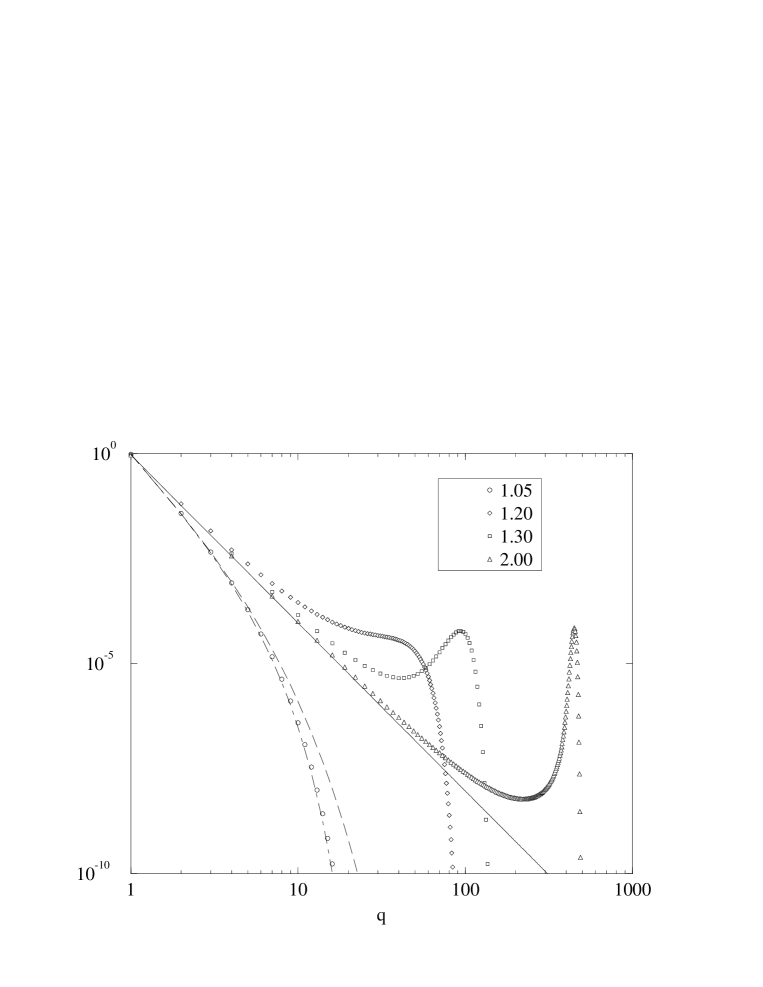
Figure 1: The effective one–point distributions for different $\rho$ and 500 boxes. The solid line is the bare distribution $p(q)\sim q^{-4}$. The finite-size corrected $\pi(q)$ distribution for $\rho=1.05$ is given by the dot-dashed line, while the long dashed line is the thermodynamical limit.

Using both these methods one confirms the following picture of the system: In the fluid phase the distribution nicely converges to the limiting distribution (16) as expected. In the condensed phase the distribution follows the limiting power-like distribution (17) for smaller $q$ but develops a peak in the tail. These effects are clearly seen on the figure 1 which illustrates the phase transition produced by change in balls density.

One can include the finite size effects into the formula (16) by noting that $\mu$ depends on $\rho$ and hence on $q$ since $\rho=(M-q)/N$. The predicted distribution is plotted on the figure 1 (dashed line) and the agreement with the exact result is excellent. The same reasoning can be applied to the formula (17). This results in sharp decrease of distribution at large $q$, clearly indicating a different nature of finite size effects in this case.

The peak in the tail appears as the system tries to compensate for the particles missing from (20). We can approximately predict the position of this peak by the following reasoning: The number of missing particles is

$$N(\rho-\sum_{q}q\pi(q))=N\left(\rho-\frac{F^{\prime}(1)}{F(1)}\right)=N(\rho-\rho_{c})$$ (22)

so assuming that all the missing particle are in one box this is the position of the peak, which as moves linearly with increasing $N$. In figure 2 we plot the position of the peak compared with prediction (22). As one can see, the agreement is excellent.

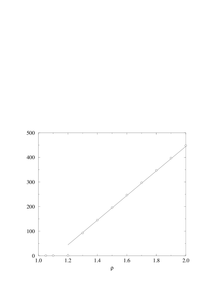
Figure 2: Position of peak as the function of $\rho$. ($\beta=4.0$, 500 boxes)

Discussion

The density driven transition obviously has a strong similarity to Bose-Einstein condensation [11], especially as presented in, for instance, [12]. Although this is usually formulated in a grand canonical ensemble with a chemical potential the discussion may be paraphrased into language very similar to that used above. If one fixes the number of energy levels to $N$ and the number of particles to $M=\rho N$ the partition function for Bose particles is

$$Z=\sum_{q_{1},\ldots,q_{N}}\prod_{i=1}^{N}\exp(-\beta q_{i}\epsilon_{i})\;\delta(\sum_{i=1}^{N}q_{i}-M)$$ (23)

where each box has its own energy level $\epsilon_{i}$. If one slips into a continuum language the expression one arrives at for the particle density (in three dimensions) is just

$$\tilde{\rho}=s\left({mkT\over 2\pi h^{2}}\right)^{{3\over 2}}F(z)$$ (24)

where $\tilde{\rho}$ is now the particle density per unit volume, $s$ is a spin degeneracy factor and $F(z)=\sum_{q=1}^{\infty}q^{-3/2}z^{q}$. At fixed particle density per unit volume $z$ is pushed to one as $T$ is reduced, at which point a sizeable proportion of the particles begin to condense in the ground state. Thus at the formal level the mechanism for the Bose-Einstein condensation and the transition discussed in this paper are identical, namely, a Dirichlet series is pushed to the limit of its radius of convergence. The similarities with the treatment of the spherical model phase transition in [13] are also apparent. In that case too the (spherical) constraint is exponentiated and a saddle point “sticking” signals the phase transition.

We would like to stress, however, that in spite of formal similarity there exists a substantial difference. In the Bose-Einstein condensation case each box has its own energy level and the energy is linear in number of balls. The system condenses into the lowest state. In the Backgammon case the boxes are equivalent and condensation is a kind of symmetry breaking process. Moreover, the energy of the box is not linear in number of balls which is absolutely crucial for existence of phase transition, so there is no direct interpretation in terms of occupied states. One way of looking at the model would be to imagine a set of $N$ “atoms” and $M$ “electrons”. The electrons would be bound to the atoms and the energy of an atom with $n$ electrons would be $\log(n)$, corresponding to the energy levels $E(k)=1/k$.

Variations of the model with different vertex weights can also be easily accommodated into the saddle point approach. For instance, changing the weight of a vertex of order $q$ from $1/q^{\beta}$ to $t_{q}/q^{\beta}$ gives the following equation for the critical density

$$\rho_{c}={\zeta(\beta-1)+q\left({t_{q}-1\over q^{\beta}}\right)\over\zeta(\beta)+\left({t_{q}-1\over q^{\beta}}\right)}.$$ (25)

For univalent vertices we can see from the above that as $t_{1}\rightarrow 0$ the asymptote for $\rho_{c}$ moves from one to two, so we reproduce the result of [7] that the transition is suppressed for finite $\beta$ when $\rho=2$.

In the case of infinite radius of convergence of $F(z)$ the condensation does not take place. Clearly, this will happen when we restrict the number of balls that are allowed in one box ($p(q)=0,\;q>q_{\mbox{max}}$) as the function $F(z)$ is then a polynomial in $z$.

The appearance of the $\zeta$ function in the saddle point equation also encourages one to play number-theoretic games with the vertex weights. It is possible to regard the standard $\zeta$ function as a bosonic partition function and define “arithmetic” k-parafermions [17] with the use of a generalized Möbius function

$$\mu_{k}(q)=1\;\;\mbox{if}\;\;q=\prod_{i}(p_{i})^{r_{i}},\;0\leq r_{i}\leq k-1$$ (26)

where the $p_{i}$ are the prime factors of $q$. The case $k=2$ corresponds to arithmetic fermions and $k=\infty$ to bosons (the standard $\zeta$ function). If the vertex weights are taken to be $\mu_{k}(q)/q^{\beta}$ the saddle point equation becomes

$$\rho=\left[{\zeta(\beta-1)\over\zeta(\beta)}-{\zeta(k\beta-1)\over\zeta(k\beta)}\right].$$ (27)

The sort of fermionic partition functions generated here are thus not useful for suppressing a collapse transition. The vertex weights do not suppress large numbers of particles in a box, only those numbers with $k$ identical prime factors are not allowed. The behaviour of $\rho_{c}$ as a function of $\beta$ is thus not much changed, apart from the asymptote for large $\beta$ being reduced to zero. These arithmetic parafermion models thus crumple at a lower $\rho_{c}$ for a given $\beta$.

The backgammon models are perhaps best thought of as models for the transition in 4D gravity at the level of baby universes and their connecting “necks” [9], identifying the polymer structure with the baby universe tree. As was noted in [9], the 4D simulations have a fluctuating density, as (almost) fixing $N_{4}$ still allows $N_{0}$ and hence $\rho$ to vary, but such a smearing of the density should not affect the saddle point equations and the resulting phase structure. The appearance of models with $p(q)\sim q^{-\beta}$ is not, as we have noted above, restricted to those arising in the context of discretized gravity simulations. In the model described in [14] the power exponent is generated dynamically and is calculated by assuming that the distribution function is properly normalised. This corresponds exactly to our constraint (20). This constraint is satisfied by a pure power law distribution only at the transition.

The backgammon models of [10] were originally formulated to investigate glassy behaviour, and their dynamics display many spin-glass like features. Although the energy landscape of the polymer inspired backgammon models here is a long way from that of the “golf-course” landscape of the original backgammon models it might still be a worthwhile exercise to investigate the dynamics of the polymer backgammon models in the light of the results of [10]. The dynamics may prove as interesting as the static properties discussed in this paper.

Appendix A

In this appendix we describe in detail the mapping between the branched polymer model of [7] and the balls–in–boxes model.

Let $n_{q}$ be the number of boxes with $q$ balls in it. These numbers must satisfy the constraints:

$$\sum_{q}n_{q}=N,\qquad\sum_{q}qn_{q}=M$$ (28)

The number of configurations with given $n_{q}$’s is given by (we assume $0!=1$)

$$\frac{N!}{n_{0}!n_{1}!\cdots n_{N}!}$$ (29)

so the partition function (1) can be written as:

$$Z(N,M)=\sum_{\{n_{i}\}}\frac{N!}{n_{0}!n_{1}!\cdots n_{N}!}p_{0}^{n_{0}}p_{1}^{n_{1}}p_{2}^{n_{2}}\cdots p(n)^{n_{N}}$$ (30)

where the sum runs over all sequences of positive integers satisfying (28).

The number of rooted, planted, planar trees with $v_{1}$ vertices of degree one, $v_{2}$ vertices of degree two, and so on is given by (see for example [16]):

$$\frac{1}{N}\frac{N!}{v_{1}!\cdots v_{N}!}$$ (31)

These numbers satisfy

$$\sum_{q}v_{q}=N,\qquad\sum_{q}qv_{q}=2N-1$$ (32)

We see that the weight of a branch polymer depends on the vertex orders in the same way as a balls–in–boxes configuration depend on the box occupation numbers[6, 7]. Therefore the BP partition function can be also written in the form (30) with the factor (29) substituted by (31). If we now forbid the empty boxes by putting $p(0)=0$ and set $M=2N-1$ ($\rho=2$) those two functions will be equivalent.

References

- [1] J. Ambjørn, “Quantization of geometry”, Les Houches 62, [hep-th/9411179]
-
[2]
J. Ambjørn, D. Boulatov, A. Krzywicki and S. Varsted,
Phys. Lett. B276 (1992) 432;
B. Brugmann and E. Marinari, Phys. Rev Lett. 70 (1993) 1908; J. Math Phys. 36 (1995) 6340. S. Catterall, J. Kogut and R. Renken, Phys. Lett. B328 (1994) 277;
J. Ambjørn and S. Varsted, Phys. Lett. B266 (1991) 285;
J. Ambjørn, Z. Burda, J. Jurkiewicz and C.F. Kristjansen, Acta Phys. Pol. B23 (1992) 991. -
[3]
P. Bialas, Z. Burda, A. Krzywicki and B. Petersson,
Nucl. Phys. B 472 (1996) 293;
B. de Bakker, “Further evidence that the transition of 4D dynamical triangulation is first oder”, [hep-lat/9603024]. - [4] T. Hotta, T. Izubuchi and J. Nishimura, Nucl. Phys. B (Proc. Suppl.), 47 (1995) 609.
- [5] S. Catterall, J. Kogut, R. Renken and G. Thorleifsson , Nucl.Phys. B468 (1996) 263.
- [6] J. Ambjørn, B. Durhuus, J. Fröhlich, P. Orland Nucl. Phys. B270 (1986) 457.
- [7] P. Bialas and Z. Burda, “Phase Transition in Fluctuating Branched Geometry”, [hep-lat/9605020], to appear in Phys. Lett. B.
- [8] J. Ambjørn and J. Jurkiewicz, Phys. Lett. B278 (1992) 42.
- [9] P. Bialas, Z. Burda, B. Petersson and J. Tabaczek, “Appearance of Mother Universe and Singular Vertices in Random Geometries”, [hep-lat/9608030].
-
[10]
F. Ritort, Phys. Rev. Lett. 75 (1995) 1190,
[cond-mat/950481];
F. Ritort and S. Franz, Europhys Lett. 31 (1995) 507, [cond-mat/9505115];
F. Ritort and S. Franz, “Glassy mean field behaviour of the backgammon model”, [cond-mat/9508133];
C. Godreche, J.P. Bouchaud and M. Mezard, J. Phys A28, (1995) L603;
C. Godreche and J.M. Luck, J. Phys A29 (1996) 1915. -
[11]
M. van den Berg, J.T. Lewis and J.V. Pulé, Helvetica Physica Acta 59 (1986) 1271;
R.M.Ziff, G.E. Uhlenbeck and M. Kac, Phys. Rep. C4 (1977) 169. - [12] R. Feynman, “Statistical Mechanics”, Benjamin/Cummings 1976.
- [13] T. Berlin and M. Kac, Phys. Rev. 86 (1952) 821.
- [14] M. Levy and S. Solomon, “Power Laws are Logarithmic Boltzmann Laws”, [hep-lat 9607001].
- [15] T. Apostol, “Introduction to Analytic Number Theory”, Springer-Verlag 1976.
- [16] I. P. Goulden, D. M. Jacson “Combinatorial Enumeration”, John Wiley & Sons 1983
- [17] I. Bakas and M. Bowick, J. Math. Phys. 32 (1991) 1881.