[

Phase Diagram of the Two Dimensional Lattice Coulomb Gas

Abstract

We use Monte Carlo simulations to map out the phase diagram of the two dimensional Coulomb gas on a square lattice, as a function of density $\rho$ and temperature T. We find that the Kosterlitz-Thouless transition remains up to higher charge densities than has been suggested by recent theoretical estimates.

]

The nature of phase transitions in the two dimensional neutral Coulomb gas (CG) has remained a topic of considerable interest. The CG can be related via duality transformation to the 2D XY model, and thus to superfluid and superconducting films.[1] The pioneering work of Kosterlitz and Thouless[2] (KT) showed that, at low charge density, there is a second order transition from an insulating to a conducting phase, due to the unbinding of neutral charge pairs. As the charge density is increased, several authors[3, 4, 5, 6] have predicted that this KT transition should become first order. Recently, Levin et al.[5], using a modified Debye-Hückel approach, have estimated that, for a continuum CG, the KT transition ends in a tricritical point at the surprisingly low density of $\rho_{\rm c}\simeq 0.004/a^{2}$, where $a$ is the hard core diameter of the charges.

To investigate this issue, we report here on new Monte Carlo simulations of the 2D CG on a square lattice, computing the phase diagram as a function of density and temperature. We make sensitive tests of the nature of the transition, and conclude that it remains second order up to densities much higher than estimated by Levin et al.

Our work follows that of Lee and Teitel,[7] with a few modifications. We take for the Hamiltonian,

$${\cal H} = {\scriptstyle{1\over 2}}\sum_{i,j}n_{i}G^{\prime}({\bf r}_{i}-{\bf r}_{j})n_{j}-u\sum_{i}n_{i}^{2}$$ (1)

$$+ \sum_{i}(n_{i}^{4}-n_{i}^{2})+V\left({2\pi P_{x}\over L}\right)+V\left({2\pi P_{y}\over L}\right)\enspace,$$ (2)

where the sums are over all sites $i$, $j$ of a 2D periodic $L\times L$ square lattice, with unit grid spacing. $G^{\prime}({\bf r})\equiv G({\bf r})-G(0)$, where $G({\bf r})$ is the solution to the lattice Laplacian with periodic boundary conditions. For $r\ll L$, $G^{\prime}({\bf r})\simeq-\ln r-{\scriptstyle{1\over 2}}\ln(8{\rm e}^{2\gamma})$, where $\gamma\simeq 0.5772$ is Euler’s constant.[2, 8] $n_{i}=0,\pm 1,\pm 2\ldots$ are the integer charges, and neutrality $\sum_{i}n_{i}=0$ is imposed. The third term in ${\cal H}$ tends to suppress charges with $|n_{i}|>1$, and is needed to stabilize the system in the very dense limit. Assuming therefore that all charges satisfy $|n_{i}|\leq 1$, so that $|n_{i}|=n_{i}^{2}$, the second term is just $-u\rho L^{2}$ with $\rho=L^{-2}\sum_{i}|n_{i}|$ the charge density. Thus $u$ is the chemical potential. The last two terms in ${\cal H}$ are effective boundary terms, which arise in the duality mapping to the CG from the 2D XY model with periodic boundary conditions.[9, 10, 11] Here ${\bf P}\equiv\sum_{i}n_{i}{\bf r}_{i}$ is the net dipole moment of the charges, and $V(\phi)$ is the Villain function,[12] $\rm{e}^{-V(\phi)/T}\equiv\sum_{m=-\infty}^{\infty}\rm{e}^{-{1\over 4\pi T}(\phi-2\pi m)^{2}}$. With these boundary terms, it is easy to compute[9, 11] the inverse dielectric tensor $\epsilon^{-1}_{\mu\nu}$, which is the equivalent of the helicity modulus of the corresponding XY model,[13, 14]

$$\epsilon^{-1}_{\mu\nu} = 2\pi\left\langle V^{\prime\prime}\left({2\pi P_{\mu}\over L}\right)\right\rangle\delta_{\mu\nu}$$ (3)

$$- {2\pi\over T}\left\langle V^{\prime}\left({2\pi P_{\mu}\over L}\right)V^{\prime}\left({2\pi P_{\nu}\over L}\right)\right\rangle\enspace,$$ (4)

where $V^{\prime}$ and $V^{\prime\prime}$ are first and second derivatives of $V$. For an isotropic system, $\epsilon^{-1}_{\mu\nu}=\epsilon^{-1}\delta_{\mu\nu}$. According to the KT instability criterion,[2] in the insulating phase we must have the inequality $\epsilon^{-1}\geq 4T$. This will enable us to set an upper bound on the transition to the conducting phase.

We carry out standard Metropolis Monte Carlo simulations for various values of $u$ and $T$. At each point an initial 20,000 MC passes are discarded to equilibrate with an additional 128,000 MC passes to compute averages. Errors are estimated from block averages.

The $u-T$ phase diagram, as found previously by Lee and Teitel,[7] is shown in Fig. 1. At low $u$, upon increasing $T$, there is a KT transition to a conducting liquid. At low $T$, upon increasing $u$, there is a first order transition to an insulating charge solid at $u_{0}=\pi/8$. Increasing $T$ within this charge solid gives first a KT transition to a conducting solid, followed by an Ising melting of the solid. The two KT lines meet the first order line at the same $T^{*}\simeq 0.125$, slightly lower than the tricritical point where the first order and Ising lines meet.

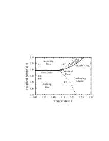
FIG. 1.: Phase diagram of the CG in the $u-T$ plane.

In Fig. 2, we present our new results for this phase diagram in the $\rho-T$ plane.

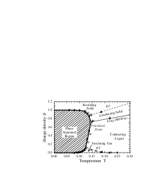
FIG. 2.: Phase diagram of the lattice CG in the $\rho-T$ plane. Open symbols are from simulations with system size $L=16$; solid symbols are from $L=32$.

The coexistence boundary is determined as follows. The low temperature branches are obtained by simulating with $u$ just above and just below $u_{0}$, measuring the average density $\rho$ as $T$ increases. To determine the boundary closer to the tricritical point, we simulate with fixed $u>u_{0}$, increasing $T$, and measuring the histogram of the values of $\rho$ found at each value of $T$. When one is in either the solid or the liquid phase, this histogram has a single peak. However, when one crosses the first order line, this histogram develops double peaks.[15] The locations of the two peaks determine the densities of the two coexisting phases. In Fig. 3 we show an example of such histograms. Varying $u>u_{0}$ then maps out the rest of the coexistence boundary.

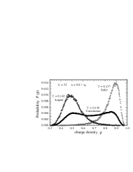
FIG. 3.: Histograms of charge density $\rho$ for $u=0.4$ just above $u_{0}=\pi/8$. At the coexistence boundary the histogram is bimodal

In Fig. 2 we show the coexistence boundary found in this way from simulations with $L=16$ and $L=32$. As is seen, and as is expected, our results near the tricritical point are limited by finite size effects. However it is clear that the KT line at small $u$ joins the first order line at a density $\rho\simeq 0.1$, much larger than the estimate of Levin et al.

Next we verify that what we have called the “KT” line at small $u$ actually does remain a second order KT transition all the way up to the first order line separating the insulating gas and insulating solid. To locate the transition temperature $T^{*}$ for $u=0.39$, just below $u_{0}$, we compute $\epsilon^{-1}(T)$ for various $L$, using Eq. (4). Our results are shown in Fig. 4. The intersection of these curves with the line $4T$ determines the upper bound $T^{*}\simeq 0.125$. No hysteresis, or other suggestion of a first order transition was observed in $\epsilon^{-1}$.

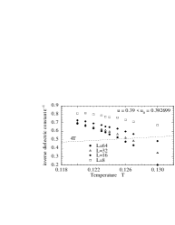
FIG. 4.: Inverse dielectric function $\epsilon^{-1}(T)$ for various lattice sizes $L$, for $u=0.39$ just below $u_{0}=\pi/8$. The intersection with the line $4T$ gives the KT upper bound on the transition temperature $T^{*}$.

As a more precise test that the transition is indeed KT–like, we use the finite size scaling procedure of Weber and Minnhagen [16, 17]. Precisely at the KT transition temperature, the finite size dependence of $\epsilon^{-1}$ is given by,

$$\epsilon^{-1}(L)=\epsilon^{-1}(\infty)\left[1+{1\over 2\ln L+c}\right]$$ (5)

Fitting data for various $L$ at fixed $T$ to Eq.(5), with $\epsilon^{-1}(\infty)$ and $c$ as free parameters, one determines $T_{\rm KT}$ as that temperature which gives the smallest $\chi^{2}$ error of the fit. The fitted value of $\epsilon^{-1}(\infty)$ at the $T_{\rm KT}$ so determined, should then turn out to be precisely $\epsilon^{-1}(\infty)=4T_{\rm KT}$, so as to obey the universal KT prediction. We show the results of such a fit below. In Fig. 5$a$ we show the $\chi^{2}$ of the fit versus temperature, where we have included sizes $L=8-64$, $12-64$, and $16-64$ in the fit. In each case, the minimum of $\chi^{2}$ occurs at $T^{*}=0.1235$. In Fig. 5$b$ we show the corresponding fitted value of $\epsilon^{-1}(\infty)/T$ versus temperature. We see that $\epsilon^{-1}(\infty)/T=4$ at essentially the same $T^{*}$ where $\chi^{2}$ has its minimum. This analysis strongly supports the transition as being of the KT type.

FIG. 5.: Fitting of $\epsilon^{-1}(T,L)$ to Eq.(5). ($a$) shows the $\chi^{2}$ of the fit vs. $T$, ($b$) shows the value of the fitted $\epsilon^{-1}(\infty)/T$ vs. $T$.

Finally, in Fig. 6 we show histograms of the density $\rho$ for $u=0.39$ and several values of $T$ passing through $T^{*}$, for the largest system size we have studied, $L=64$. We have chosen the values of $T$ shown in Fig. 6 so that the histograms between neighboring values have a significant overlap. As is clearly seen, all the distributions are single peaked. There is no sign at all of the bimodal distribution that would characterize a first order transition. While we cannot rule out the possibility of a weak first order transition with a $\xi(T^{*})>64$, our results clearly suggest that the “KT” line at small $u$ does indeed remain a second order Kosterlitz-Thouless transition all the way up to $u_{0}$.

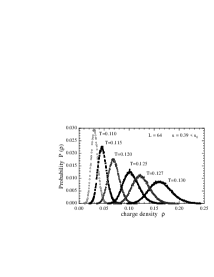
FIG. 6.: Histograms of charge density $\rho$ for $u=0.39$ just below $u_{0}=\pi/8$. Histograms remain single peaked as one passes though the transition at $T^{*}\simeq 0.1235$

Our lattice simulation has the advantage that it is easier to equilibrate at high densities than continuum simulations. However the presence of the discrete lattice does have a strong influence on the location of the phase boundaries. In particular, the coexistence boundary of Fig. 2 at small $T<0.1$ is well described by a simple model of excited isolated dipoles and quadrupoles. For the lower branch we get $\rho_{-}(T)={1\over L^{2}}(2N_{d}{\rm e}^{-\beta E_{d}}+4N_{q}{\rm e}^{-\beta E_{q}})$, where $E_{d}$ and $E_{q}$ are the excitation energies of an isolated dipole and quadrupole respectively, and $N_{d}=4L^{2}$ and $N_{q}=2L^{2}$ are the number of ways of putting them down on the square lattice. For the upper branch we get $\rho_{+}(T)=1-{1\over L^{2}}(2N^{\prime}_{d}{\rm e}^{-\beta E^{\prime}_{d}}+4N^{\prime}_{q}{\rm e}^{-\beta E^{\prime}_{q}})$ where $E^{\prime}_{d}$ and $E^{\prime}_{q}$ are the energies for removing an isolated dipole and quadrupole, and $N^{\prime}_{d}=2L^{2}$ and $N^{\prime}_{q}=L^{2}$ are the number of ways this may be done. Clearly these expressions will change with the geometry of the discretizing lattice, or if a continuum is used. Nevertheless, at the very low densities $\rho\sim 0.004$ and high temperatures $T\simeq 0.25$ where Levin et al. estimate a tricritical point, we would be very surprised if the lattice is qualitatively different from the continuum.

Using a discrete lattice also has the effect that it tends to stabilize the charge solid phase above $u_{0}$ to high temperatures. Indeed, our charge solid only melts after it has already become conducting via a KT transition arising from the excitation and diffusion of vacancies throughout the solid. The present model does not possess any first order transition from an insulating to a conducting phase. In contrast, recent simulations[18, 19] of the CG in a flat continuum with periodic boundary conditions find that the charge solid phase is melted at any finite temperature. Here, a first order line separates the insulating gas from a dense conducting liquid, ending at a critical point at relatively low temperature and high density: $(T_{c},\rho_{c})=(0.056,0.21)$ according to Ref. [18], and $T_{c}=0.032$ according to Ref. [19]. Similar results were found earlier for the continuum CG on the surface of a sphere:[20] $(T_{c},\rho_{c})=(0.087,0.11)$. In these models, the KT line ends either at, or near this critical point.

Although the geometry of the the CG system clearly affects the location of the end of the KT transition line, it is interesting to compare our results for the square lattice with the predictions of the continuum self-consistent screening theory of Minnhagen and Wallin.[3] To do so, it is necessary to note[2, 8] that if the interaction $G(\vec{r})$ on the lattice is chosen so as to asymptotically match the continuum $-\ln r$ as $r\to\infty$, then the lattice CG with $u=0$ acts like a continuum model with a chemical potential $\mu_{0}=-{1\over 4}\ln(8{\rm e}^{2\gamma})\simeq 0.8085$. Thus a chemical potential $u_{0}=\pi/8$ on the grid acts like a chemical potential $\mu=u_{0}-\mu_{0}=-0.416$ in the continuum. Minnhagen and Wallin predict that the KT line will end at $T^{*}=0.144$ and fugacity $z^{*}=0.054$, giving a chemical potential $\mu=T^{*}\ln z^{*}=-0.420$.

To conclude, we show that the 2D neutral CG continues to have an ordinary KT transition up to high densities $\rho\sim 0.1$, in contrast with recent theoretical estimates. This result, obtained here for the square lattice CG, is consistent with recent simulations in the continuum.

One of us (PG) would like to thank Calin Ciordas for interesting discussions and the Department of Physics of the University of Rochester for a teaching assistantship. This work was supported by U.S. Department of Energy grant DE-FG02-89ER14017.

REFERENCES

- [1] For a review see, P. Minnhagen, Rev. Mod. Phys. 59, 1001, (1987).
- [2] J. M. Kosterlitz and D.J.Thouless, J. Phys. C 6, 1181 (1973); J. M. Kosterlitz, ibid. 7, 1046 (1974).
- [3] P. Minnhagen and M. Wallin, Phys. Rev.B 36, 5620 (1987); ibid. 40, 5109 (1989).
- [4] J. M. Thijssen and H. J. F. Knops, Phys. Rev. B 38 9080 (1988).
- [5] Y. Levin, X. Li and M. E. Fisher, Phys.Rev.Lett. 73, 2716 (1994).
- [6] M. Friesen, Phys. Rev.B 53, R514, (1996).
- [7] J.-R. Lee and S. Teitel, Phys. Rev. B 46, 3247 (1992).
- [8] J. V. José, L. P. Kadanoff, S. Kirkpatrick, and D. R. Nelson, Phys Rev. B 16, 1217 (1977).
- [9] A. Vallat and H. Beck, Phys. Rev. B 50, 4015 (1994).
- [10] H. S. Bokil and A. P. Young, Phys. Rev. Lett. 74, 3021 (1995).
- [11] P. Olsson, Phys. Rev. B 52, 4511 (1995).
- [12] J. Villain, J. Physique 36, 581, (1975). Note that the coupling in our definition has an extra factor of as compared to the conventional definition.
- [13] T. Ohta and D. Jasnow, Phys. Rev. B 20, 130 (1979).
- [14] P. Minnhagen and G. G. Warren, Phys. Rev. B 24, 2526 (1981).
- [15] J. Lee and J. M. Kosterlitz, Phys. Rev. Lett. 65, 137 (1990).
- [16] H. Weber and P. Minnhagen, Phys. Rev. B 37, 5986 (1988).
- [17] A similar analysis in Ref. [7], as applied to the finite wavevector , is in error, as pointed out by Olsson in Ref. [11].
- [18] G. Orkoulas and A. Z. Panagiotopoulos, J. Chem. Phys. 104, 7205 (1996).
- [19] J. Lidmar and M. Wallin, preprint cond-mat/9607025.
- [20] J. M. Caillol and D. Levesque, Phys. Rev. B 33, 499 (1986).