Deconfined Fermions but Confined Coherence?

Abstract

The cuprate superconductors and certain organic conductors exhibit transport which is qualitatively anisotropic, yet at the same time other properties of these materials strongly suggest the existence of a Fermi surface and low energy excitations with substantial free electron character. The former of these features is very difficult to account for if the material possesses three dimensional coherence, while the latter is inconsistent with a description based on a two dimensional fixed point. We therefore present a new proposal for these materials in which they are categorized by a fixed point at which transport in one direction is not renormalization group irrelevant, but is intrinsically incoherent, i.e. the incoherence is present in a pure system, at zero temperature. The defining property of such a state is that single electron coherence is confined to lower dimensional subspaces (planes or chains) so that it is impossible to observe interference effects between histories which involve electrons moving between these subspaces.

I Motivation

Interest in the physics of strongly correlated, anisotropic materials has undergone a resurgence since the discovery of the cuprate superconductors. One of the central questions in the theory of these materials is the question of under what circumstances, if any, real bulk materials exhibit effective dimensionalities other than three. The question is certainly an important one in the under and optimally doped cuprates because they exhibit qualitatively anisotropic transport. For example, the temperature dependence of the $c$-axis resistivity in under and optimally doped La_2-xSr_xCuO₄ is nonmetallic at low temperatures [1], while the $ab$ conductivity remains metallic essentially all the way down to $T_{c}$. YBa₂Cu₃O_6+x and Bi₂Sr₂CaCu₂O₈ exhibit activated $c$ axis conduction at low temperatures, with $ab$ transport again remaining metallic [2]. Meanwhile, the frequency dependent conductivity is perhaps even more anomalous with no signs of anything remotely like a Drude peak with any appreciable weight in the $c$-axis conductivity in either underdoped YBa₂Cu₃O_6+x [3] or La_2-xSr_xCuO₄ [4]. In fact, $c$-axis conduction is rather generically incoherent in these materials and has anomalous temperature dependence in a range near to $T_{c}$. This is difficult to understand given that the scale of the expected $c$-axis bandwidth from ab initio band structure calculations is typically 2000K [5].

Interaction effects can clearly reduce this and one might attempt to explain some of the anomalies in the $c$-axis conduction in terms of a reduced $c$-axis bandwidth. Indeed, it is in principle possible for sufficiently strong interactions to result in some non-Fermi liquid (NFL) in plane state with respect to which the out of plane hopping would be an irrelevant perturbation and this might help to explain some of the transport anomalies. However, the criterion for the renormalization group irrelevance of the interplane hopping is that

$$\lim_{\Lambda\rightarrow 0}\Lambda^{2}\gg\lim_{\Lambda\rightarrow 0}\int_{0}^{\Lambda}\int_{0}^{\omega}\int_{0}^{\omega}d\omega d\omega_{1}d\omega_{2}\delta(\omega-\omega_{1}-\omega_{2})\rho_{e}(k_{F}+0^{+},\omega_{1})\rho_{h}(k_{F}+0^{-},\omega_{2})$$ (1)

where $\rho_{e}(k_{F}+0^{+},\omega_{1})$ is the spectral function for inserting an electron with momentum just outside the Fermi surface and $\rho_{h}(k_{F}+0^{-},\omega_{2})$ is the spectral function for creating a hole with momentum just inside the Fermi surface. The requirement is clearly violated if either the electron and hole spectral function diverges at zero temperature and frequency on the Fermi surface, with the other either diverging or remaining finite. In fact, the photoemission data [6, 7] show a sharp quasiparticle peak at temperatures above $T_{c}$ and it appears pathological to assume that the peak does not narrow arbitrarily on the Fermi surface as $T\rightarrow 0$, except for impurity effects which will not affect the renormalization group status of the hopping, $t_{\perp}$, unless the impurity scattering rate is large compared to the renormalized hopping, $t_{\perp}^{R}$. There is also no theoretical reason for a particle-hole anisotropy strong enough to cause the hole spectral function to vanish, and it therefore appears highly unlikely that $t_{\perp}$ is renormalization group irrelevant. It might be possible for $t_{\perp}^{R}$ to remain finite, but small enough that even a temperature of 40 Kelvin might be taken to be high compared to the $c$-axis bandwidth. However, in that case, one expects to be able to describe the conductivity in terms of hopping conduction and one expects:

$$\sigma_{c}(\omega)\propto\frac{1}{\omega}\sum_{k}\int d\epsilon\rho(k,\epsilon)\rho(k,\epsilon+\omega)\left(n_{f}(\epsilon)-n_{f}(\epsilon+\omega)\right)$$ (2)

This predicts a Drude peak at low frequency given the form of the spectral function observed in the photoemission, but no such peak is seen.

This does not constitute an experimental proof that something very peculiar is going on regarding the dimensional crossover in the cuprates, but it is certainly suggestive. What seems to be required is a fixed point at which $t_{\perp}^{R}$ is not zero, or even particularly small, and yet conduction is somehow very different from the usual, three dimensional case. It is the purpose of this work to make a specific proposal for such a fixed point: a state in which coherent transport is intrinsically confined to the planes, despite the fact that the electrons themselves are not [18, 19]. In this state a material would not be three dimensional in the usual sense, but neither would it be purely two dimensional.

II A Simple Model of Coupled Non-Fermi Liquids

Unfortunately, our understanding of 2D NFL states is not well enough developed to permit precise calculations to be made. However, it is possible to consider the analogous problem in one less dimension, where we understand the Luttinger liquid [8, 9] behavior of interacting fermions. We therefore consider the problem of Luttinger liquids coupled by interliquid single particle hopping as a potential paradigm for coupled NFL’s [10].

This problem is far from new: as early as 1974, in the context of the newly discovered quasi-1D organic conductors, Gorkov and Dzyaloshinskii discussed how various key properties of a 1D electron “chain” could be destroyed by the presence of interchain hopping [11]. Many other authors have since addressed the problem, using various techniques [12]. To our knowledge, however, ours is the only approach which directly addresses the question of interliquid coherence. This question is of crucial importance, for many of the other approaches begin with an anisotropic 2D electron gas (or its two chain analogue), a state with manifestly coherent interliquid hopping, upon which interactions are treated perturbatively. In those approaches which do not begin with the anisotropic 2D electron gas, we believe that, while in some cases unreasonable approximations and/or errors have been made, in general, these works have all correctly demonstrated the relevance of $t_{\perp}$ but have simply not addressed the question of its coherence. In general, past workers have argued that the flow away from $t_{\perp}=0$ should lead to higher dimensional coherence and, for infinitely many chains, to a Fermi liquid or to some other (CDW, SDW or BCS) known higher dimensional fixed point, mainly because of the lack of an alternative proposal. We are proposing the confinement of coherence as such an alternative.

The key construct needed in investigating the nature of interliquid hopping is the electron spectral function, $\rho(k,\omega)$:

$$\rho(k,\omega) = \theta(\omega)\rho^{+}(k,\omega)+\theta(-\omega)\rho^{-}(k,-\omega)$$ (3)

$$= \sum_{n}\left\{\theta(\omega)|\langle n_{N+1}|c_{k}^{{\dagger}}|0_{N}\rangle|^{2}\delta(\omega-E_{n}^{N+1})+\theta(-\omega)|\langle n_{N-1}|c_{k}|0_{N}\rangle|^{2}\delta(\omega-E_{n}^{N-1})\right\}$$ (4)

In a FL, $\rho(k,\omega)$ is dominated by a term which sharpens up to a $\delta$-function as $k\rightarrow k_{F}$. This term, of weight $Z_{k}\neq 0$, is the quasiparticle part of $\rho(k,\omega)$. The remainder of $\rho(k,\omega)$ is featureless so that, as far as low energy properties are concerned, only the quasiparticle part of $\rho(k,\omega)$ matters. If $\langle i,j\rangle$ label physically adjacent liquids, and $k$ in-liquid momenta, then an interliquid hopping term of the form

$\displaystyle H_{\perp}=t_{\perp}\sum_{\langle i,j\rangle,k}\left(c_{i,\sigma}^{{\dagger}}(k)c_{j,\sigma}(k)+{\rm h.c.\/}\right)$

will directly couple a quasiparticle state in one liquid with an energy degenerate quasiparticle state in the physically adjacent liquids. In this case, we should be doing degenerate perturbation theory and starting with interliquid Bloch states of precise interliquid momenta. An interliquid band will therefore form, entailing a coherent interliquid velocity and hence coherent interliquid transport.

In contrast, in a Luttinger liquid (or any NFL, by definition) there are no Landau quasiparticles. The quasiparticle weight, $Z_{k}$, is zero, but in a nontrivial way. The Luttinger liquid spectral function differs from that for a FL in that its singularities are power law in nature, even at the Fermi surface. For the physically most relevant case of spin-independent electronic interactions, $\rho(k,\omega)$ has singularities at $\omega=\pm v_{c}k,v_{s}k$ determined by a single exponent $\alpha$, and $v_{c}$ and $v_{s}$ denote velocities of propagation of charge and spin currents. We believe that this could potentially lead to the confinement of coherence to the individual Luttinger liquids. To see how this might come about, let us begin with simple model within which to discuss quantum coherence and incoherence: a two level system (TLS) coupled to a dissipative bath.

III Incoherence and the Two Level System

To begin with we define, following Ref. [13], the two level system model with the Hamiltonian:

$$H_{\rm TLS}=\frac{1}{2}\Delta\sigma_{x}+\sum_{i}\left(\frac{1}{2}m_{i}\omega_{i}x_{i}^{2}+\frac{1}{2m_{i}}p_{i}^{2}\right)+\frac{1}{2}\sigma_{z}\sum_{i}C_{i}x_{i}$$ (5)

Here $C_{i}$ is the coupling to the $i$th oscillator, and $m_{i}$, $\omega_{i}$, $x_{i}$ and $p_{i}$ are the mass, frequency, position and momentum of the $i$th oscillator, respectively.

We restrict our discussion of the model to zero temperature and the the so called ohmic regime [13] where the spectral density of the bath is given by:

$$J(\omega) = \frac{\pi}{2}\sum_{i}\frac{C_{i}}{m_{i}\omega_{i}}\delta(\omega-\omega_{i})$$ (6)

$$= 2\pi~{}\alpha~{}\omega\exp(-\omega/\omega_{c})$$ (7)

$\alpha$ is a positive constant measuring the strength of the coupling to the bath and $\omega_{c}$ is a cutoff frequency.

The model describes a single quantum mechanical degree of freedom which can be in either of two states and which is coupled to a bath of harmonic oscillators. The environment, represented by the bath of oscillators, influences the tunneling because the bath is sensitive to which of the states the spin is in. Hereafter we will refer to the discrete degree of freedom as a “spin” for convenience. This is appropriate since we are describing the spin with Pauli matrices.

The model provides the prototypical example of a quantum to classical crossover since, for $C_{i}=0$ the model represents the quantum mechanics of an isolated two state system, whereas for sufficiently strong coupling to the environment the dynamics of the spin, if followed without reference to the oscillator bath, are dissipative and no quantum coherence effects are observable [13]. In fact, this is how one generally expects classical behavior to emerge for macroscopic systems: the macroscopic degrees of freedom exchange energy with an enormous number of unobserved microscopic degrees of freedom and therefore different histories are unable to maintain a definite relative phase long enough for quantum interference effects to manifest themselves.

What sort of quantum interference effects do we expect to be able to observe in the TLS for sufficiently weak coupling to the environment? Consider a model where the coupling to the environment vanishes, i.e. $\alpha=0$, and the system is prepared in a state where the spin is in a $\sigma_{z}$ eigenstate. The exact eigenstates of the spin are the $\sigma_{x}$ eigenstates which are split by an energy $\Delta$ so that the initial state of the system is a superposition of these two states of different energy with a definite phase between the two states in the superposition. Although not constant, this relative phase remains well defined indefinitely and therefore results in observable oscillations in the expectation value of $\sigma_{z}$, in fact (in units where $\hbar=1$) $\langle\sigma_{z}(t)\rangle=\cos\Delta t$. In the TLS model the oscillations persist for a range of couplings to the environment, albeit with coupling dependent damping of the oscillations.

To study these oscillations the standard theory of the TLS focuses on a quantity called $P^{(1)}(t)$ (hereafter simply $P(t)$) which is the probability of finding the system in the $\sigma_{z}=1$ state for $t>0$ for a system which has been prepared by clamping the spin into the $\sigma_{z}=1$ state for all $t<0$, allowing the oscillator bath to relax to equilibrium in this configuration and finally releasing the spin at $t=0$. Note that calculation of $P(t)$ is equivalent to determining $\langle\sigma_{z}(t)\rangle$, since the two are simply related by $\langle\sigma_{z}(t)\rangle=2P(t)-1$. $P(t)$ is an appropriate quantity to study for questions about macroscopic quantum coherence since, if the spin represents a generic macroscopic quantum degree of freedom which the experimenter can observe and control, whereas the oscillators represent microscopic degrees of freedom which are beyond both control and observational capacities of the experimenter, it is exactly the sort of preparation used in the definition of $P(t)$ which is possible experimentally. The signature of quantum coherence in $P(t)$ will be the presence of oscillations (damped or otherwise) in contrast to the incoherent relaxation, $P(t)\sim\frac{1}{2}(1+e^{-\Gamma t})$, which results if the spin is sufficiently strongly coupled to the environment, e.g. when $\alpha>1/2$ [13].

For further discussion of the TLS problem, it is convenient to make a canonical transformation on the original model, so that the coupling to the oscillators is removed by taking:

$$H_{\rm TLS}^{\prime}=\hat{U}H_{\rm TLS}\hat{U}^{-1}$$ (8)

where

$$\hat{U}=\exp\left(-\frac{1}{2}\sigma_{z}\sum_{i}\frac{C_{i}}{m_{i}\omega_{i}^{2}}\hat{p}_{i}\right)$$ (9)

$\hat{p}_{i}$ is the momentum operator of the $i$th oscillator. The new Hamiltonian takes the form:

$$H_{\rm TLS}^{\prime}=\frac{1}{2}\Delta(\sigma^{+}e^{-i\Omega}+h.c.)+H_{\rm oscillators}$$ (10)

where $\Omega=\sum_{i}\frac{C_{i}}{m_{i}\omega_{i}^{2}}p_{i}$. The tunneling operator between the two states has been replaced by an operator which creates and destroys excitations of the oscillator bath, as well as changing the state of the spin.

In this formulation, $P(t)$ can be reinterpreted as the probability of finding $\sigma_{z}(t)=1$ for a system in which $\Delta$ is suddenly switched on at time $t=0$ with the system in the $\Delta=0$ groundstate with $\sigma_{z}=1$. The previous definition in which the spin was clamped in the $\sigma_{z}=1$ eigenstate for all negative times and the oscillators were allowed to adapt to the clamped state is equivalent. Consider, the two point correlation function of $\sigma^{+}e^{-i\Omega}$, which obeys:

$$\langle\sigma^{+}e^{-i\Omega(t)}\sigma^{-}e^{i\Omega(0)}\rangle = \exp\left\{-\int_{0}^{\infty}\frac{1-e^{-i\omega t}}{\omega^{2}}J(\omega)\right\}$$ (11)

$$= \exp\left\{-2\alpha\int_{0}^{\infty}\frac{1-e^{-i\omega t}}{\omega}e^{-\omega/\omega_{c}}\right\}$$ (12)

$$\sim e^{i\pi\alpha}(\omega_{c}t)^{-2\alpha}$$ (13)

With the correlation function we can immediately construct the spectral function of the operator $e^{i\Omega}$ in the low energy, universal regime:

$$\rho_{\Omega}(\omega) = \sum_{m}|\langle m|e^{i\Omega}|GS\rangle|^{2}\delta(\omega-E_{m})$$ (14)

$$= \Gamma^{-1}(2\alpha)~{}\theta_{+}(\omega)~{}\omega^{-1+2\alpha}\omega_{c}^{-2\alpha}\exp(-\omega/\omega_{c})$$ (15)

where $\{m\}$ is a complete set of oscillator eigenstates with energies $E_{m}$ and $|GS\rangle$ is the oscillator ground state. The spectral function is normalized to integrate to unity since $\langle e^{-i\Omega(t)}e^{i\Omega(t)}\rangle=1$.

The short time approximation to $P(t)$ can be constructed straightforwardly using the spectral function above and ordinary time dependent perturbation theory. We find:

$$P(t)=1-\frac{\Delta^{2}}{2}\int d\omega\rho_{\Omega}(2\omega)\frac{\sin^{2}(\omega t)}{\omega^{2}}+\cdots$$ (16)

Notice that when $\alpha>1$, $\rho_{\Omega}(\omega)\sim\omega^{-1+2\alpha}$ results in an infrared convergent $P(t)$; in the limit $\Delta\rightarrow 0$, $P(t)\rightarrow 1$ for all $t$. This corresponds to the irrelevance of $\Delta$ and the localization of the spin predicted by Chakravarty and Bray and Moore [14] based on a mapping of the TLS to the inverse squared Ising model.

Conversely, for $\alpha\rightarrow 0$, $\rho_{\Omega}(\omega)\rightarrow\delta(\omega)$ and $P(t)=1-\frac{\Delta^{2}}{4}t^{2}+...$, in agreement with the expansion of the exact result $P(t)=(1+\cos\Delta t)/2$. For $0<\alpha<1$ we are in a more complicated region. Clearly the difference between $P(t)$ and $1$ grows to order unity for any arbitrarily small $\Delta$ throughout this region (the simply reflects the renormalization group relevance of $\Delta$) and one would at first sight be tempted to conclude that throughout this region $P(t)$ would undergo damped oscillations with a period approximately given by $t_{\rm osc}$, where $t_{\rm osc}$ satisfies:

$$1=\frac{\Delta^{2}}{2}\int d\omega\rho_{\Omega}(2\omega)\frac{\sin^{2}(\omega t_{\rm osc})}{\omega^{2}}$$ (17)

One should be cautious, however, in view of the fact that for $\alpha>1/2$ the spectral function for the tunneling operator is vanishing at low frequencies and, at $\alpha=1/2$, it is flat and featureless out to the cutoff scale. A flat spectral function is equivalent to a featureless density of states and is exactly the condition under which the Golden Rule approximation should be valid, implying incoherent decay without any recurrence effects or oscillations. In fact, the exact solution of the TLS at the special value $\alpha=1/2$ shows purely incoherent relaxation in $P(t)$, and, while the true behavior of $P(t)$ in the region $1/2<\alpha<1$ is not rigorously known [13], there are reasons for believing that the behavior there is no more coherent. The simple reason for this is that since, in these cases the spectral function has even more high energy weight, perturbation theory in $\Delta$ is even less coherent than for $\alpha=1/2$. Incoherence is the direct result of the non-degeneracy of the perturbation theory in $\Delta$. Let us discuss this important point in more detail.

The important physical effect of finite $\alpha$ is that there is a substantial contribution to $P(t)$ from transitions to states with energies that are larger than the putative renormalized oscillation frequency, $\Delta_{R}\sim t_{\rm osc}^{-1}$ (see Eq. 17) . When the amount of weight in these transitions is larger than the amount of weight in transitions to low energy states, it no longer makes sense to consider the effects of $\Delta$ to be coherent. Effectively, each change of state, i.e. flipping of the spin, is accompanied by the creation or annihilation of a sufficient number of bosons in the environmental bath that the phase of that history is randomized compared to histories with no spin flip. Intuitively, one has crossed over from degenerate or nearly degenerate perturbation theory to non-degenerate perturbation theory (as opposed to the transition to irrelevant $\Delta$ where the long time perturbation theory becomes convergent).

To see that this picture does agree with the known TLS results, let us calculate the contribution to $P(t)$ from transitions to states with various energies. The low energy part contributes to $P(t)$ an amount

$$\delta P_{\rm low}(t) = \frac{\Delta^{2}}{2}\int_{0}^{1/t}d\omega\rho_{\Omega}(2\omega)\frac{\sin^{2}(\omega t)}{\omega^{2}}+\cdots$$ (18)

$$\sim \frac{\Delta^{2}}{2^{2-2\alpha}}t^{2-2\alpha}\Gamma^{-1}(2\alpha)~{}\frac{{}_{1}F_{2}(-1+\alpha;\frac{1}{2},\alpha;-1)-1}{4(1-\alpha)}$$ (19)

where ${}_{1}F_{2}$ is a generalized hypergeometric function [15]. This evaluates to $\frac{1}{4}\Delta^{2}t^{2}$ at $\alpha=0$ and, for $\alpha=1/2$, to $\frac{1}{4}\Delta^{2}t\,(2\,{\rm Si}(2)+\cos 2-1)\approx 0.45\Delta^{2}t$ (${\rm Si}$ is the sine integral function).

The high energy part contributes

$$\delta P_{\rm high}(t) = \frac{\Delta^{2}}{2}\int_{1/t}^{\infty}d\omega\rho_{\Omega}(2\omega)\frac{\sin^{2}(\omega t)}{\omega^{2}}+\cdots$$ (20)

$$\sim \frac{\Delta^{2}}{2^{2-2\alpha}}t^{2-2\alpha}\Gamma^{-1}(2\alpha)\left(\frac{1}{4(1-\alpha)}+\frac{\Gamma(2\alpha)\cos\pi\alpha}{2^{2\alpha}(1-2\alpha)(1-\alpha)}-\frac{{}_{1}F_{2}(-1+\alpha;\frac{1}{2},\alpha;-1)}{4(1-\alpha)}\right)$$ (21)

For $\alpha\rightarrow 0$ the high energy part vanishes like $\Gamma^{-1}(2\alpha)$ (the prefactor is $\frac{1}{4}\Delta^{2}t^{2}\left(\frac{3}{2}-\gamma-\ln 2+\frac{1}{6}~{}_{2}F_{3}(1,1;2,5/2,3;-1)\right)\approx 0.1\Delta^{2}t^{2}$), while for $\alpha=1/2$ the result is $\frac{1}{2\pi}\Delta^{2}t\,(1+\pi-_{1}F_{2}(-\frac{1}{2};\frac{1}{2},\frac{1}{2};-1)\approx 0.34\Delta^{2}t$, comparable to the low energy contribution.

Clearly, the high energy contribution is insignificant as $\alpha\rightarrow 0$ because of the divergence of $\Gamma(2\alpha)$ (the gamma function has a simple pole at $0$) and, for any arbitrary division into “high” and “low”, could always be made so by taking a suitably small $\alpha$. One therefore expects to find coherence in the limit $\alpha\rightarrow 0$. On the other hand, for finite values of $\alpha$ the high energy part can be as important as the low energy part, depending upon our division into high and low energy integrals. Using the qualitatively reasonable division above, we see that for $\alpha=1/2$ the two contributions are in fact comparable. In fact, for any division scheme involving energy scales small compared to the oscillator cutoff, the high energy part must dominate for some $\alpha<1$, since, in the limit where $\alpha\rightarrow 1$, the high energy part diverges logarithmically like $\frac{\Delta^{2}}{2\omega_{c}^{2}}\ln(\omega_{c}t)$ while the low energy part is finite and given by $\frac{\Delta^{2}}{2\omega_{c}^{2}}(\gamma+\ln(2)-{\rm Co}(2))\approx 0.85~{}\frac{\Delta^{2}}{2\omega_{c}^{2}}$, where ${\rm Co}$ is the cosine integral function and $\gamma$ is Euler’s constant. The high energy part can therefore be made arbitrarily large compared to the low energy part for any arbitrary partition into high and low energy pieces as we approach $\alpha=1$. The dominance of the high energy part does not necessarily imply that the quantum oscillations must cease entirely; it could be that the oscillations would persist but become arbitrarily heavily damped. However, when the high energy part has become of order one, the argument that oscillations should occur with a frequency $\omega_{osc}\sim\Delta_{R}$ becomes unreliable and, in fact, as we have seen above, the conclusion of the exact solution [13]) is that the oscillations vanish for $\alpha=1/2$.

The reason for the success of our perturbation theory, which is essentially a “short time expansion”, in predicting a qualitative change in the tunneling is that the expansion is valid out to precisely the time when the spin has order one probability of flipping and is therefore perfectly adequate to describe the nature of the states reached by spin flip processes. In particular, it can identify whether these states are nearly degenerate with the initial state (and each other) or of widely disparate energies, which is the essential physical question for coherence. Hence, the main conclusions of this section: the qualitative behavior of $P(t)$, in the sense of whether or not it exhibits oscillations, i.e. quantum coherence, can actually be determined from lowest order perturbation theory. The special point $\alpha=1/2$, at which the Golden Rule is naively applicable, separates a region of completely incoherent behavior, $1/2\leq\alpha<1$, from one of damped oscillations, $0<\alpha<1/2$.

IV The Connection to Fermionic Hopping

The existence of a third regime in the TLS problem with behavior qualitatively different from that occurring for irrelevant tunneling or undamped tunneling is suggestive, however, before we can claim that the lessons of the TLS have any relevance to the fermionic hopping we must make some firmer connection between the tunneling matrix element, $\Delta$, and the single particle hopping, $t_{\perp}$ between non-Fermi liquids, in our case one dimensional Luttinger liquids.

We will study this problem using bosonization techniques [8, 9]. General, gapless, one dimensional interacting electronic systems and higher dimensional Fermi liquids can both be studied via this approach so our results can be made at least that general.

The Hamiltonians of the isolated systems are of the general Luttinger liquid form:

$$H = \frac{1}{4\pi}\int dx~{}\left(v_{\rho}K_{\rho}(\partial\Theta_{\rho})^{2}+v_{\rho}K_{\rho}^{-1}(\partial\Phi_{\rho})^{2}+v_{\sigma}K_{\sigma}(\partial\Theta_{\sigma})^{2}+v_{\sigma}K_{\sigma}(\partial\Phi_{\sigma})^{2}\right)$$ (22)

$$= \frac{1}{4\pi}\int dx~{}\left(v_{\rho,N}(\partial\Theta_{\rho})^{2}+v_{\rho,J}(\partial\Phi_{\rho})^{2}+v_{\sigma,N}(\partial\Theta_{\sigma})^{2}+v_{\sigma,J}(\partial\Phi_{\sigma})^{2}\right)$$ (23)

where $K_{\rho}$ is interaction dependent and less than one for a repulsive interaction, while $K_{\sigma}$ is set to one hereafter as a consequence of considering only interactions which preserve the $SU(2)$ spin invariance. The bosonized form for the electron operator is given by

$$\Psi^{\dagger}_{\uparrow}(x)\sim\sqrt{\frac{\partial\Phi_{\uparrow}(x)}{\pi}}\sum_{m~{}odd}A_{m}~{}\exp\left(i[m\Phi_{\uparrow}(x)+\Theta_{\uparrow}(x)]\right)$$ (24)

so that the inter-liquid hopping is given by:

$$\Psi^{\dagger,(1)}_{\uparrow}(x)\Psi^{(2)}_{\uparrow}(x) \sim \sqrt{\frac{\partial\Phi^{(1)}_{\uparrow}(x)}{\pi}}\sum_{m~{}odd}A_{m}~{}\exp\left(i[m\Phi^{(1)}_{\uparrow}(x)+\Theta^{(1)}_{\uparrow}(x)]\right)$$ (25)

$$\times \sqrt{\frac{\partial\Phi^{(2)}_{\uparrow}(x)}{\pi}}\sum_{m~{}odd}A_{m}^{\star}~{}\exp\left(i[m\Phi^{(2)}_{\uparrow}(x)-\Theta^{(2)}_{\uparrow}(x)]\right)$$ (26)

where

$$\Theta_{\uparrow}=2^{-\frac{1}{2}}(\Theta_{\rho}+\Theta_{\sigma})$$ (27)

$$\Theta_{\downarrow}=2^{-\frac{1}{2}}(\Theta_{\rho}-\Theta_{\sigma})$$ (28)

and

$$\Theta_{\rho}(x)=\Theta_{\rho}^{0}+N_{\rho}x/L-i\sum_{q\neq 0}|\frac{2\pi}{qL}|^{\frac{1}{2}}K_{\rho}^{-\frac{1}{2}}~{}{\rm sgn}(q)e^{iqx}\left(b^{\dagger}_{\rho}(q)+b_{\rho}(-q)\right)$$ (29)

$$\Phi_{\rho}(x)=\Phi_{\rho}^{0}+J_{\rho}x/L-i\sum_{q\neq 0}|\frac{2\pi}{qL}|^{\frac{1}{2}}K_{\rho}^{\frac{1}{2}}~{}{\rm sgn}(q)e^{iqx}\left(b^{\dagger}_{\rho}(q)-b_{\rho}(-q)\right)$$ (30)

where the $b_{\rho}$ operators create and annihilate the bosonic, charge density eigenexcitations. Similar expressions obviously apply for $\Theta_{\sigma}$ and $\Phi_{\sigma}$. The expression for hopping of down spin electrons is easily obtained by changing the sign of $\Theta_{\sigma}$ and $\Phi_{\sigma}$ in Eq. 25, while that for hops in the other direction can be obtained by interchanging the chain labels in 25.

In the above expressions the operators $\Theta^{0}_{\uparrow}$ and $\Phi^{0}_{\uparrow}$ are canonically conjugate to the the conserved quantum numbers $J_{\uparrow}$ and $N_{\uparrow}$ and are not expressible in terms of the bosons. The role of these operators was stressed by Haldane in his solution of the Luttinger model [9], however they are generally ignored since they do not enter into single particle correlation functions. They will be crucial for our discussion since it is the quantum numbers $N$ and $J$ that are analagous to $\sigma_{z}$ in the TLS problem. This is readily apparent when the canonically transformed form for the tunneling matrix element, $\frac{\Delta}{2}\sigma^{+}e^{-i\Omega}+~{}h.c.$ (see Eq. 10), is compared to the bosonized form for the interchain hopping in Eq. 25. Both contain operators which act to raise and lower otherwise conserved quantum numbers ($\sigma_{z}$ for the TLS and $N_{\uparrow,1}-N_{\uparrow,2}$, $J_{\uparrow,1}-J_{\uparrow,2}$, etc. for the fermion hopping). In addition to the raising and lowering operators, both contain exponentials in bosonic creation and annihilation operators which are responsible for the interesting dynamics and determine the correlation functions of the operators. In fact, if the fermionic hopping occurred at only a single point in space, that problem could be mapped onto the TLS problem. We do not believe that such a mapping exists for the physical model of a uniform interchain hopping. However, the formal connection between the models is quite strong and suggests that the interesting incoherent regime for the TLS might well have a fermionic analogue.

The analogue to $P(t)$ for the fermionic problem is clear: instead of taking a system adapted to $\Delta=0$ with $\sigma_{z}=1$ and then turning on $\Delta$ suddenly, we take the groundstate of a system with some non-zero values for $N_{\uparrow,1}-N_{\uparrow,2}$, $J_{\uparrow,1}-J_{\uparrow,2}$, etc. to $t_{\perp}=0$ and then turn on $t_{\perp}$ suddenly. Instead of studying the resulting oscillations (or lack thereof) in $\sigma_{z}(t)$ we study them in $N_{\uparrow,1}(t)-N_{\uparrow,2}(t)$, etc. For simplicity we will hereafter consider only the case where the initial condition has $N_{\uparrow,1}-N_{\uparrow,2}=J_{\uparrow,1}-J_{\uparrow,2}=N_{\downarrow,1}-N_{\downarrow,2}=J_{\downarrow,1}-J_{\downarrow,2}=\delta N(t=0)\neq 0$, i.e. equal numbers of up and down spin electrons are added at the right Fermi point of one chain. We will follow the dynamics of $\langle\delta N(t\neq 0)\rangle$.

This is a somewhat unfamiliar approach to studying $t_{\perp}$ so it is worth examining the results for the simple case of free fermions. In that case, the problem is exactly soluble. The requirement that the two chains be prepared in states adapted to $t_{\perp}=0$ and in which no Tomonaga bosons are excited but in which $\delta N(t=0)\neq 0$ is easily satisfied by simply taking $n_{1,\sigma}(k)=\Theta(k_{F}-k+\frac{2\pi}{L}\delta N)\Theta(k_{F}+k)$ while $n_{2,\sigma}(k)=\Theta(k_{F}-k)\Theta(k_{F}+k)$. Since the free fermion problem is a single particle one every $k$ is independent and independent oscillations occur for the $\delta N$ states for which $n_{1,\sigma}(k)-n_{2,\sigma}(k)\neq 0$. The exact result for $\langle\delta N(t)\rangle$ is $\delta N(t=0)\cos(2t_{\perp}t)$. This is exactly analogous to the $\alpha=0$ case of the TLS and clearly corresponds to the interchain hopping being coherent. Given this coherence, it is reasonable to expect that the description based on degenerate perturbation theory in $t_{\perp}$ and symmetric and antisymmetric combinations of the fermion operators for the two chains will be appropriate.

Notice that in this sense free electrons (and also Fermi liquids although we have not shown that here) exhibit a heretofore unremarked on macroscopic quantum coherence: the total number difference between two chains (or planes) of free electrons is a macroscopic variable which would undergo oscillations, rather than incoherent relaxation, if a finite interchain hopping were suddenly turned on. Viewed in this light it is not surprising that there might exist states in which this macroscopic variable loses its coherence. Rather, it is surprising (though undoubtedly correct for all normal metals) that macroscopic quantum behavior should occur in generic materials. It is interesting that this macroscopic quantum coherence has not previously occasioned some concern in the theory of interacting electronic systems. It turns out that the arguments we have found guaranteeing the presence of coherent oscillations in Fermi liquids rely in several places on the quasiparticle structure of the Fermi liquid, which fails totally for interacting fermions in one spatial dimension. We therefore believe that the postulate of previous works on arrays of chains of interacting fermions coupled by a single particle hopping [12] that the relevance of $t_{\perp}$ signals a crossover to a three dimensionally coherent Fermi liquid is just that: a postulate. In fact, we will see that the extension to coupled Luttinger liquids of the tools we have used for the TLS problem and coupled Fermi liquids does not support the conclusion that a relevant $t_{\perp}$ is always a coherent $t_{\perp}$.

To begin our analysis of coupled Luttinger liquids, we require the spectral function of the single particle hopping operator between otherwise isolated Luttinger liquids. This is easily obtained from the spectral function of the single particle Green’s function. The universal features of this function are readily accessible [16]. At the level of a linearized dispersion relation, the annihilation operator for momentum $k$ has the same spectral function (when the Fermi energy contribution to the energies is taken out) as the creation operator for momentum $2k_{F}-k$. The hopping operator’s spectral function can be obtained by convolving the spectral function of the individual creation and annihilation operators.

For $\delta N(t=0)=0$, the spectral function for $\sum_{k}c^{\dagger}_{1}(k)c_{2}(k)$ is given by $L~{}\alpha\omega^{4\alpha}\Lambda^{-(1+4\alpha)}$ where $2\alpha=\frac{1}{4}(K_{\rho}+K_{\rho}^{-1}-2)$ is the anomalous exponent of the single particle Green’s function for the case with spin and $2\alpha=\frac{1}{2}(K_{\rho}+K_{\rho}^{-1}-2)$ for the spinless case. Since the spectral function vanishes as $\omega\rightarrow 0$ the response to $t_{\perp}$ is always incoherent for $\delta N(t=0)=0$. This should not be surprising since for $\delta N(t=0)=0$ there is no possibility of coherent oscillations in $\langle\delta N(t)\rangle$. It is for this reason that for free particles there would be no response for $\delta N(t=0)=0$ since their response is entirely coherent. Fermi liquids would have a response but there would be no long time singular behavior, the single quasiparticle hopping having been completely blocked for $\delta N(t=0)=0$.

Notice that for the Luttinger liquid, the long time incoherent response is singular provided that $4\alpha<1$, despite the fact that coherent hopping is totally blocked. This suggests that in some sense incoherent hopping is relevant and that flows away from the $t_{\perp}=0$ fixed point may be dominated by this relevant operator, rather than the relevant operator corresponding to coherent interliquid hopping. If this is the case, then the renormalization group flows should end elsewhere than Fermi liquid theory. This is due not only to the anomalous exponent of the Luttinger liquid, but also the destruction of the Fermi surface. No such effect would be present for a model with a single particle Green’s function of the form $G(k,\omega)\sim(\omega-vk)^{-1+2\alpha}$.

$\langle\delta N(t)\rangle$ is the natural quantity to study for coherence effects, however, we will not be able to go beyond lowest order in perturbation theory (which should still be sufficient for settling questions of coherence as we argued in the TLS case) and here the behavior of $\langle\delta N(t)\rangle$ can be misleadingly coherent because it involves the subtraction of the contributions from the hops in different directions. Clearly, if the hopping in both directions is incoherent, then any coherence in the difference is an artifact. It is therefore useful to consider the quantity $P(t)$, defined as the probability to remain in the initial state:

$$P(t) = |\langle O|\exp(i\int_{0}^{t}dt^{\prime}H^{\prime}(t^{\prime}))|0\rangle|$$ (31)

$$\sim 1-4t_{\perp}^{2}\int d\omega\frac{\sin^{2}(\omega t/2)}{\omega^{2}}\left(\rho_{1\rightarrow 2}(\omega)+\rho_{2\rightarrow 1}(\omega)\right)+\dots$$ (32)

Note that oscillations in $\delta N$ are the natural signature of coherence and no oscillatory behavior in $P(t)$ is expected in general; however it is useful for the above reasons to now restrict ourselves to $P(t)$.

Let us now procede with a short time expansion analogous to that which we used for the TLS. This should be valid for determining the presence or absence of coherence for exactly the same reason as it was for that problem: the presence or absence of coherence is equivalent to the near degeneracy or non-degeneracy of the states connected to the initial state by $t_{\perp}$. The short time expansion is capable of revealing such features since it is valid out to precisely the timescale where the initial state has been left behind.

For spinless fermions and finite $\delta N(t=0)$ ($k_{F}^{1}>k_{F}^{2}$) the initial spectral function for $\sum_{k}c^{\dagger}_{1}(k)c_{2}(k)$ is given by:

$$\rho_{2\rightarrow 1}(\omega) = \Gamma^{-1}(2\alpha)\Gamma^{-1}(2+2\alpha)(2v_{S})^{-(1+4\alpha)}\Theta\left(\omega-(E_{F}^{1}-E_{F}^{2})-v_{S}(k_{F}^{1}-k_{F}^{2})\right)$$ (34)

$$\left(\omega-(E_{F}^{1}-E_{F}^{2})-v_{S}(k_{F}^{1}-k_{F}^{2})\right)^{1+2\alpha}\left(\omega-(E_{F}^{1}-E_{F}^{2})+v_{S}(k_{F}^{1}-k_{F}^{2})\right)^{-1+2\alpha}$$

likewise

$$\rho_{1\rightarrow 2}(\omega) = \Gamma^{-1}(2\alpha)\Gamma^{-1}(2+2\alpha)(2v_{S})^{-(1+4\alpha)}\Theta\left(\omega-(E_{F}^{1}+E_{F}^{2})-v_{S}(k_{F}^{1}-k_{F}^{2})\right)$$ (36)

$$\left(\omega-(E_{F}^{2}-E_{F}^{1})-v_{S}(k_{F}^{1}-k_{F}^{2})\right)^{-1+2\alpha}\left(\omega-(E_{F}^{2}-E_{F}^{1})+v_{S}(k_{F}^{1}-k_{F}^{2})\right)^{1+2\alpha}$$

$P(t)$ is radically different, even at small $\alpha$ from the Fermi liquids case. In fact for small $\delta N(t=0)$, the incoherent part of the spectral function (high energy) completely dominates $P(t)$ and may destroy coherence completely, if the incoherent (high energ) hops effect the coherent (low energy) ones. One way to disentangle the coherent and incoherent competition is to consider the spectral functions broken down into the contributions coming from individual momenta. First, examine the spectral function for $c^{\dagger}_{1}(k)c_{2}(k)$, which may be obtained by convolving the spectral functions for $c^{\dagger}_{1}(k)$ and $c_{2}(k)$. The spectral function for $c^{\dagger}_{1}(k)$ has support for $\omega>E_{F}^{1}+v_{S}|k-k_{F}^{1}|$, where $v_{S}$ is the sound velocity of the Luttinger liquid. The spectral function behaves at large $\omega$ like

$$\rho_{\dagger,1}(\omega~{}large)\sim\omega^{-1+2\alpha}$$ (37)

and behaves for $\omega\rightarrow E_{F}^{1}+v_{S}|k-k_{F}^{1}|$ like

$$\rho_{\dagger,1}(\omega~{}small)\sim\left(\omega-(E_{F}^{1}+v_{S}|k-k_{F}^{1}|)\right)^{\alpha-H(k-k_{F}^{1})}$$ (38)

where $H(x)=1$ if $x\geq 0$ and $O$ if $x\leq 0$. The integrated weight is $1-n_{1}(k)$. The spectral function for $c_{2}(k)$ has support for $\omega>-E_{F}^{2}+v_{S}|k-k_{F}^{2}|$, also behaves at large $\omega$ like

$$\rho_{2}(\omega~{}large)\sim\omega^{-1+2\alpha}$$ (39)

and behaves for $\omega\rightarrow~{}-E_{F}^{2}+v_{S}|k-k_{F}^{2}|$ like

$$\rho_{2}(\omega~{}small)\sim\left(\omega-(v_{S}|k-k_{F}^{2}|-E_{F}^{2})\right)^{\alpha-H(k_{F}^{2}-k)}$$ (40)

The integrated weight is $n_{2}(k)$.

The convolution has support for $\omega>E_{F}^{1}-E_{F}^{2}+v_{S}|k-k_{F}^{1}|+v_{S}|k-k_{F}^{2}|$ which means that except for $k_{F}^{2}\leq k\leq k_{F}^{1}$ the threshold is $E_{F}^{1}-E_{F}^{2}+2v_{S}|k-k_{F}^{avg}|$ where $k_{F}^{avg}=(k_{F}^{1}+k_{F}^{2})/2$. The behavior as $\omega\rightarrow E_{F}^{1}-E_{F}^{2}+2v_{S}|k-k_{F}^{avg}|$ is

$$\rho_{\dagger,1,2}(\omega~{}small)\sim\left(\omega-E_{F}^{1}-E_{F}^{2}+2v_{S}|k-k_{F}^{avg}|\right)^{4\alpha}$$ (41)

For the case, where $k_{F}^{2}\leq k\leq k_{F}^{1}$, the threshold is smallest; there the $k$ independent threshold is given by

$$\omega_{min}(k) = E_{F}^{1}-E_{F}^{2}+v_{S}(k-k_{F}^{2})-v_{S}(k-k_{F}^{1})$$ (42)

$$= E_{F}^{1}-E_{F}^{2}+v_{S}(k_{F}^{1}-k_{F}^{2})$$ (43)

$$> 0$$ (44)

The behavior of the spectral function as $\omega\rightarrow E_{F}^{1}-E_{F}^{2}+v_{S}(k_{F}^{1}-k_{F}^{2})$ is

$$\rho_{\dagger,1,2}(\omega~{}small)\sim\left(\omega-E_{F}^{1}-E_{F}^{2}+v_{S}(k_{F}^{1}-k_{F}^{2})\right)^{1+4\alpha}$$ (45)

The positivity of the minimum energy results and the large exponent with which the spectral function vanishes result from the fact that hops in this direction are ‘wrong way’ hops, that is they increase rather than decrease the initial $\delta N$.

The behavior for large $\omega$ is given by

$$\rho_{\dagger,1,2}(\omega~{}large)\sim\omega^{-1+4\alpha}$$ (46)

The integrated weight is $(1-n_{1}(k))n_{2}(k)$.

The spectral function for $c^{\dagger}_{2}(k)c_{1}(k)$ is similar. The spectral function for $c^{\dagger}_{2}(k)$ has support for $\omega>E_{F}^{2}+v_{S}|k-k_{F}^{2}|$ behaves at large $\omega$ like

$$\rho_{\dagger,2}(\omega~{}large)\sim\omega^{-1+2\alpha}$$ (47)

and behaves for $\omega\rightarrow E_{F}^{2}+v_{S}|k-k_{F}^{2}|$ like

$$\rho_{\dagger,2}(\omega~{}small)\sim\left(\omega-(E_{F}^{2}+v_{S}|k-k_{F}^{2}|)\right)^{\alpha-H(k-k_{F}^{2})}$$ (48)

The integrated weight is $1-n_{2}(k)$. The spectral function for $c_{1}(k)$ has support for $\omega>-E_{F}^{1}+v_{S}|k-k_{F}^{1}|$, also behaves at large $\omega$ like

$$\rho_{1}(\omega~{}large)\sim\omega^{-1+2\alpha}$$ (49)

and behaves for $\omega\rightarrow~{}-E_{F}^{1}+v_{S}|k-k_{F}^{1}|$ like

$$\rho_{1}(\omega~{}small)\sim\left(\omega-(v_{S}|k-k_{F}^{1}|-E_{F}^{1})\right)^{\alpha-H(k_{F}^{1}-k)}$$ (50)

The integrated weight is $n_{1}(k)$.

The convolution has support for $\omega>E_{F}^{2}-E_{F}^{1}+v_{S}|k-k_{F}^{1}|+v_{S}|k-k_{F}^{2}|$ which means that except for $k_{F}^{2}\leq k\leq k_{F}^{1}$ the threshold is $E_{F}^{2}-E_{F}^{1}+2v_{S}|k-k_{F}^{avg}|$. The behavior as $\omega\rightarrow E_{F}^{2}-E_{F}^{1}+2v_{S}|k-k_{F}^{avg}|$ is

$$\rho_{\dagger,2,1}(\omega~{}small)\sim\left(\omega-E_{F}^{2}-E_{F}^{1}+2v_{S}|k-k_{F}^{avg}|\right)^{4\alpha}$$ (51)

For the case, $k_{F}^{2}\leq k\leq k_{F}^{1}$ threshold is $E_{F}^{2}-E_{F}^{1}+v_{S}(k_{F}^{1}-k_{F}^{2})$, which vanishes for weak interactions and is always smaller than the threshold for hops in the other direction. The behavior as $\omega\rightarrow E_{F}^{2}-E_{F}^{1}+v_{S}(k_{F}^{1}-k_{F}^{2})$ is

$$\rho(\omega~{}small)\sim\left(\omega-(E_{F}^{2}-E_{F}^{1}+v_{S}(k_{F}^{1}-k_{F}^{2}))\right)^{-1+2\alpha}$$ (52)

There is a power law divergence. The behavior for large $\omega$ is given by

$$\rho_{\dagger,2,1}(\omega~{}large)\sim\omega^{-1+4\alpha}$$ (53)

The total weight in the spectral function is given by $n_{1}(k)(1-n_{2}(k))$.

In the region where $k_{F}^{2}\leq k\leq k_{F}^{1}$ a Fermi liquid spectral function would be a delta function at zero frequency, but here there is a power law singularity at a non-zero, negative frequency since $E_{F}^{1}-E_{F}^{2}=(k_{F}^{1}-k_{F}^{2})\frac{v_{J}+v_{N}}{2}$ is always larger than than $v_{S}(k_{F}^{1}-k_{F}^{2})=\sqrt{v_{J}v_{N}}(k_{F}^{1}-k_{F}^{2})$ [17]. The essential points are that the singularity is in general not at zero energy and is a power law rather than a delta function.

Notice that when $4\alpha>1$, none of the spectral functions for the individual momenta is decreasing for large $\omega$. The high energy behavior is thus incoherent which implies that the response in the $t_{\perp}\rightarrow 0$ limit is always incoherent at every $k$ at short times. The low energy behavior for $\delta N(t=0)=0$ is also incoherent. This implies that the proposal of incoherence for $\alpha^{>}_{-}1/4$ is self-consistent, since incoherence leads to a vanishing oscillation frequency, $\omega_{\rm osc}$, and therefore the natural $k_{F}^{1}-k_{F}^{2}$ to consider is $\omega_{\rm osc}/v_{F}=0$, a case where all the spectral functions are in fact incoherent. Notice that for $\alpha<1/4$ this consistency is not present since even for $k_{F}^{1}-k_{F}^{2}=0$, some of the spectral functions associated with momenta near to the Fermi surface are coherent. The self-consistency is therefore not trivial and we believe that there is incoherence for all $\alpha>1/4$. Moreover, we can rule out the possibility that the incoherent phase is pushed all the way to $\alpha=1/2$, where irrelevance sets in. This cannot occur because, as $\alpha$ approaches $1/2$, the high energy piece is diverging relative to the low energy, just as in the TLS problem.

There remains the question of the effect of higher order terms on these arguments. The only physically significant effect at higher order is interactions among the hopped fermions which intuitively should be detrimental to coherence, pushing it to lower values of $\alpha$ than $1/4$. For coherence to be restored at higher order, the initial spectral functions for the initial hops would have to have been gross misrepresentations of the spectral functions for later hops. There is no reason at all for believing that this occurs, but we have been unable rigorously include such high order processes.

If the fermionic hopping is incoherent and $\langle\delta N\rangle$ does not oscillate, then the implications of this for the physics of such a system should be dramatic. If we follow the usual assumption of the TLS problem, then the absence of interference effects in $\langle\delta N\rangle$ implies that interference effects in general should not be observable in such a system for histories which involve fermionic hopping between the Luttinger liquids. The presence of a higher dimensional Fermi surface for many chains or two split Fermi surfaces for two chains are the direct result of such interference effects and one expects that they will not result in the incoherent regime. It is for this reason that the incoherent regime must constitute a totally different fixed point from states where the coherence is not confined to the $ab$ plane - the shape of the Fermi surface provides an order parameter which distinguishes the two phases in the low energy, long time limit. All of these qualitative features can clearly be carried over to a higher dimensional analog where non-Fermi liquid chains are coupled incoherently.

In this case, there should be a host of strange physical properties associated with the incoherence. The temperature dependence of the conductivity is a difficult problem from this point of view and it is not clear that the activated behavior seen in underdoped YBa₂Cu₃O_6+x and Bi₂Sr₂CaCu₂O₈ can be explained by incoherence alone. It more likely results from the presence of some other relevant operator such as an interplane $J$. However, the incoherence proposal seems to work remarkably well for the other experimental results. For instance, we expect an optical conductivity in the $c$ direction which exhibits no Drude peak at low frequencies and rises weakly with frequency at high frequencies [20]. The idea of confined coherence is at least consistent with all of the know behaviors of $c$ axis transport in the cuprates, and, in particular, it is consistent with the peculiarly contradictory features discussed in Section I. However, the greatest experimental support for the proposal comes from experiments on an anisotropic organic conductor, (TMTSF)₂PF₆. As we will now discuss, this material directly exhibits a low temperature phase in which interference effects between histories involving interplane hops are totally absent [21]!

V Incoherence in (TMTSF)₂PF₆

(TMTSF)₂PF₆ is a highly anisotropic organic conductor. The material is triclinic and the three real space lattice directions are denoted by $a$, $b$ and $c$, respectively, with the hopping integrals in the three different directions estimated to be approximately $250~{}meV$,$25~{}meV$ and $1~{}meV$. The Coulomb energy to put two electrons in the same unit cell is estimated at about $1eV$, so that the material should be strongly correlated as well as highly anisotropic. This is especially true in light of the fact that the conduction band of the material is half-filled at low temperatures due to a dimerization and the fact that the anisotropy is so large that the corresponding Fermi surface should be topologically one dimensional, consisting of a pair of warped Fermi sheets.

Reflecting the strong correlation effects, the low temperature phase diagram of the material is quite rich: the material is in a spin density wave state at ambient pressure and temperatures below about 12 Kelvin, but becomes either superconducting (below about 1K) or metallic (at higher temperatures) on the application of pressure. In addition, in high magnetic fields and pressures there is a cascade of field induced spin density wave transitions [22]. For our purposes, we are interested in the metallic phase that occurs above about 6 kilobars of pressure and above 1 Kelvin (in zero field) or at lower temperatures in applied magnetic fields of a few Tesla. In this region the material exhibits highly anomalous magnetoresistance behavior [23] (see Figure 1)

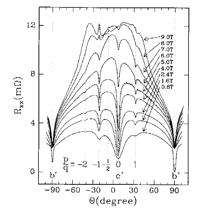
FIG. 1.: Resistance along the most conducting direction (in milliohms) as a function of magnetic field strength and orientation. Field was rotated in the $bc$ plane and angle $\Theta$ is defined so that $\pm$90 degrees coincide with the $b$ direction. Data are taken from Ref. 21

Specifically, for the resistivity measured either in the most conducting direction, parallel to $a$, or in the least conducting direction, perpendicular to the $ab$ planes, resistivity is a strong function of magnetic field strength and orientation. For a material with isotropic scattering and a topologically one dimensional Fermi surface, the magnetoresistance in the most conducting direction vanishes identically, so the greater than fivefold increases possible in the resistivity are highly surprising. It is not believed that the effect can be accounted for by an anisotropic scattering rate with any reasonable assumptions about the electron-electron interaction [24].

In addition to the anomalously large magnitude of the magnetoresistance, there is also a striking angular dependence with sharp minima occurring whenever the magnetic field parallels a real space lattice vector. These features are referred to as “Lebed magic angles”, following a suggestion of Lebed’s that there should be features in the fields induced spin density wave transition for fields with these orientations [22]. There are a number of theoretical proposals to account for the presence of these commensurability features [25], however, we will see that a magnetic field induced confinement of coherence to the $ab$ planes will provide a very natural one, and one which leads to a number of strong, and strikingly confirmed, predictions.

The scenario we envision is the following: due to the strong correlation and large anisotropy, conduction in the $c$ direction in (TMTSF)₂PF₆ is nearly incoherent and, in this sense, the material is nearly two dimensional. In this case it is important that an applied magnetic field with a component perpendicular to the $ac$ plane will render hopping in the $c$ direction somewhat inelastic. To see this inelasticity, one encorporates the field via a Peierls substitution, in which case, one finds that the states connected by the hopping no long have the same momentum in the $a$ directions but rather differ in momentum by $\frac{el_{c}H_{b}}{c}$, and since there is a well defined $v_{F}^{a}$ due to the topologically one dimensional Fermi surface, the states connected by hopping in the $c$ direction will have their degeneracy lifted by $\frac{el_{c}H_{b}v_{F}^{a}}{c}\sim H_{b}\cdot 0.2meV/Tesla$. This added inelasticity will enhance the non-degeneracy of the perturbation theory in $t_{c}$, the hopping in the $c$ direction, and if conduction were nearly incoherent before, the field may drive the material into the purely incoherent regime. This effect clearly won’t occur if the magnetic field is purely in the $c$ direction, and one expects the resistivity to dip sharply there. The out of $ab$ plane resistivity should have the strongest dip near $c$ since it is precisely the conduction in that direction that is changing character at the transition; however, the transition should be also be associated with a large change in the $a$ resistivity, since the material is really changing between two different states, and the scattering effects in the incoherent state ought to be more pronounced due to an effectively reduced dimensionality. This can clearly explain the angle dependence of the magnetoresistance around $c$ and, for any substantial hopping integrals in the $\hat{c}\pm\hat{b}$ direction, the dips associated with those directions as well, however, the real strength of the theory lies in the other predictions that it leads to.

One immediate prediction is that the minimum in the magnetoresistance associated with fields parallel to $b$ has a different origin than the other minima: it is not associated with the restoration of coherence and is therefore not a magic angle effect. This difference is readily apparent in the data for resistivity in the $a$ direction where the magnetoresistance has a cusp like behavior at $b$. Moreover, the value of the magnetoresistance for fields in the $b$ direction is field independent above 1 Tesla, while this is not true of the other minima. It is important to note that the change in resistivity out of the $ab$ planes is only order one for large fields directed along $b$. If the magnetic fields were somehow rendering the interplane hopping irrelevant then we would not expect the a much larger change in the resistivity than this at temperatures of 0.5 Kelvin and we would not expect any saturation of the magnetoresistance. Likewise a Fermi liquid explanation of the resistivity out of the $ab$ planes predicts no saturation of the resistivity for this field orientation. The observed behavior really only makes sense if there is a large incoherent hopping that is relatively unaffected by the magnetic field and a small coherent hopping that is wiped out by the field.

Let us now discuss the behavior away from $b$ and from the magic angles. The field strength independence for fields oriented along $b$ is a direct consequence of the most powerful prediction of the incoherence explanation of the magic angles behavior: the scaling of the magnetoresistance. Since the incoherent regime is categorized by the impossibility of observing interference effects between histories in which particles leave the $ab$ planes, it is clear that, neglecting Zeeman effects and treating the magnetic field again at the level of a Peierls substitution, all physical properties should be independent of the magnetic field components that lie in the $ab$ plane. This is because in a path integral calculation of any physical quantity, these components of the fields enter through a phase factor proportional to the flux enclosed by these paths that leave the $ab$ plane. This phase, however, must be unimportant if interference effects between these paths are blocked by the incoherence. The magnetoresistance in the $a$ direction should therefore demonstrate a kind of scaling behavior away from the magic angle dips, so that if the resistance is replotted versus only the component of the field out of the $ab$ plane, then the curves obtained by rotation of fields of different strengths should all lie on top of each other. Such a plot is shown in Figure 2 and the extent to which the results satisfy the prediction is striking.

FIG. 2.: Magnetoresistance along the most conducting direction (in milliohms) as a function of the square root of the component of the magnetic field perpendicular to the $ab$ plane. As explained in the text, the data are expected to scale away from the magic angle dips. Data taken from Ref. 21

Even more striking is the scaling of the resistance out of the $ab$ plane shown in Figure 3, since in this case the resistance depends only on the component of the magnetic field parallel to the current!

FIG. 3.: Log of the resistance along the least conducting direction (in ohms) as a function of log (base 10) of the component of the magnetic field (in Tesla) perpendicular to the $ab$ plane. As explained in the text, the data are expected to scale away from the magic angle dips. Raw data were provided by Danner, et al..

In both cases, the magnetoresistance depends on the field through some anomalous power law: $\Delta R\propto(\vec{H}\cdot\hat{n}_{ab})^{x}$ with $x\sim 1/2$ for resistivity in the $a$ direction and $x\sim 3/2$ for resistivity in the $c$ direction. We are not able to calculate the form of the scaling functions that our theory predicts at the present time, however, the presence of such anomalous power laws is broadly compatible with the picture of incoherently coupled non-Fermi liquid plans, while these anomalous powers are not compatible with any of the previous proposals to account for the magic angles behavior [25].

This scaling should only occur away from the magic angles and for sufficiently large fields, since otherwise the material is three dimensionally coherent. The points taken from the central magic angle dip in Figure 2 clearly violate the scaling exactly as we expect, so the prediction is satisfied at that level. The low field anisotropy in the magnetoresistance is currently being investigated by Chaikin et al. [26] and the prediction that it should not satisfy the scaling that occurs in the incoherent regime will thus be tested in the near future; the present evidence is that the scaling is violated in exactly the manner expected at low fields.

Danner, et al. [27] have also investigated the coherence question in (TMTSF)₂PF₆ directly using a novel resonance in the $c$ axis conductivity discovered by them [28]. The resonance is a Fermi liquid effect associated with the averaging of the $c$ axis velocity to zero in a magnetic field due to the quasiclassical trajectories over the Fermi surface. It should therefore be present in (TMTSF)₂PF₆ only in the coherent regions. This is exactly what is found by Danner, et al. experimentally [27].

There is thus ample experimental evidence that (TMTSF)₂PF₆ undergoes a transition in magnetic field at low temperatures to a state in which coherent transport is confined to the $ab$ planes of the material. The effect is more pronounced in cleaner samples and at lower temperatures (thus ruling out impurity- or thermally-induced incoherence) and, we believe, provides direct experimental evidence for the existence of a new fixed point with interaction induced confinement of the coherence.

REFERENCES

- [1] Y. Nakamura and S. Uchida, Phys. Rev. B 47, 8369 (1993).
- [2] N. P. Ong, Physica C 221, 235 (1994).
- [3] S. L. Cooper, P. Nyhus, D. Reznik, M. V. Klein, W. C. Lee, D. M. Ginsberg, B. W. Veal, A. P. Paulikas and B. Dabrovski, Phys. Rev. Lett. 70, 1533 (1993).
- [4] K. Tamasaku, T. Ito, H. Takagi and S. Uchida, Phys. Rev. Lett. 72, 3088 (1994).
- [5] P. B. Allen, W. E. Pickett and H. Krakauer, Phys. Rev. B 37, 7482 (1988).
- [6] H. Ding et al., Phys. Rev. Lett., 74, 2784 (1995); 76, 1533 (1996).
- [7] D. S. Dessau, (thesis) Stanford University, 1992.
- [8] A. Luther and I. Peschel, Phys. Rev. B12, 3908 (1975).
- [9] F. D. M. Haldane, J. Phys. C 14, 2585 (1981).
- [10] The notion of intrinsic incoherent transport resulting from interactions is clearly more general than the model we have considered, and our calculation is really meant to establish that such incoherence is possible. More generally, we can expect it to occur for sufficiently strong interactions if the system, for , (1) is gapless, (2) lacks the quasiparticle structure of a Fermi liquid and (3) lacks a sharp Fermi surface (not necessarily implied by 2).
- [11] L. P. Gorkov and I. E. Dzyaloshinski, Sov. Phys. JETP 40, 198 (1974).
- [12] X.G. Wen, Phys. Rev. B 42, 6623 (1990); C. Bourbonnais and L. G. Caron, Int. J. Mod. Phys. B 5, 11033 (1991); H.J. Schulz, Int. J. Mod. Phys B 5, 57 (1991); M. Fabrizio, A. Parola and E. Tosatti, Phys. Rev. B 46, 3159 (1992); F. V. Kusmartsev, A. Luther and A. Nersesyan, JETP Lett. 55, 692 (1992); C. Castellani, C. di Castro and W. Metzner, Phys. Rev. Lett. 69, 1703 (1992); V. M. Yakovenko, JETP Lett. 56, 5101 (1992); A. Finkelshtein and A. I. Larkin, Phys. Rev. B 47, 10461 (1993); A. A. Nersesyan, A. Luther and F. V. Kusmartsev, Phys. Lett. A 176, 363 (1993); D. Boise, C. Bourbonnais and A. M. S. Tremblay, Phys. Rev. Lett. 74, 968 (1995).
- [13] A. J. Leggett, S. Chakravarty, A. T. Dorsey, M. P. A. Fisher, A. Garg and W. Zwerger, Rev. Mod. Phys. 59, 1 (1987)
- [14] S. Chakravarty, Phys. Rev. Lett. 49, 681 (1982) ; A. J. Bray and M. A. Moore, Phys. Rev. Lett. 49, 1546 (1982).
- [15] I. S. Gradshteyn and I. M. Ryzhik, Tables of Integrals, Series and Products (Academic, New York, 1980).
- [16] V. Meden and K. Schönhammer, Phys. Rev. B 46, 15753 (1992); J. Voit, Phys. Rev. B 47, 6740 (1993); S. P. Strong, condmat/9410058.
- [17] Here we considered a at only the right Fermi point, if we add equal numbers at both Fermi points then , which is again in general different from but may be smaller if the interaction is attractive.
- [18] D. G. Clarke, S. P. Strong and P. W. Anderson, Phys. Rev. Lett. 72, 3218 (1994).
- [19] D. G. Clarke and S. P. Strong, Ferroelectrics 177, 1 (1996).
- [20] D. G. Clarke, S. P. Strong and P. W. Anderson, Phys. Rev. Lett. 74, 4499 (1995).
- [21] S. P. Strong, D. G. Clarke and P. W. Anderson, Phys. Rev. Lett. 73, 1007 (1994).
- [22] L. P. Gorkov and A. G. Lebed, J. Physique Lett. 45, 433 (1984).
- [23] W. Kang, S. T. Hannahs and P. M. Chaikin, Phys. Rev. Lett. 69, 2827 (1992).
- [24] V. M. Yakovenko and A. Zhelezhyak, Procedings of the International Conference on the Science and Technology of Synthetic Metals, Syn. Metals 69-71 (1994).
- [25] P. M. Chaikin, Phys. Rev. Lett. 69, 2831 (1992); K. Maki, Phys. Rev. B 45, 5111 (1992); T. Osada, S. Kagoshima and N. Miura, Phys. Rev. B 46, 1812 (1992); A. G. Lebed, J. Phys. I France 4, 351 (1994).
- [26] P.M. Chaikin, K. Chashechkina and G. M Danner, unpublished.
- [27] G. M. Danner and P. M. Chaikin, Phys. Rev. Lett. 75, 4690 (1995).
- [28] G. M. Danner and P. M. Chaikin, Phys. Rev. Lett. 72, 3714 (1994).