The phase diagram of high-$T_{c}$’s: Influence of anisotropy and disorder

Abstract

We propose a phase diagram for the vortex structure of high temperature superconductors which incorporates the effects of anisotropy and disorder. It is based on numerical simulations using the three-dimensional Josephson junction array model. We support the results with an estimation of the internal energy and configurational entropy of the system. Our results give a unified picture of the behavior of the vortex lattice, covering from the very anysotropic Bi₂Sr₂CaCu₂O₈ to the less anisotropic YBa₂Cu₃O₇, and from the first order melting ocurring in clean samples to the continuous transitions observed in samples with defects.

I Introduction

The phase diagram of high temperature superconductors in the mixed state has provided an astonishingly broad field to workers in -among other fields- many body problems, polymer physics, low dimensional systems, critical phenomena, and statistical physics in general. The main reason of this situation is the great number of parameters that define the behavior of the vortex structure. On the other hand, the same abundance of parameters defining the system turns difficult to find a unified description of all features observed in experiments. Some of the main parameters that define the behavior of the vortex structure are the external magnetic field $H$, temperature $T$, anisotropy $\eta$, and the disorder (which produces a non-homogeneous pinning potential for the vortices) that at this moment we loosely characterize by a parameter $D$. There are convincing explanations of the main characteristics of different sectors of this multi-dimensional phase diagram, such as the first order melting of the vortex-lattice in clean samples, the continuous melting of a glassy phase in disordered samples, or the existence of two different superconducting transitions (perpendicular and parallel to $H$) in some cases (for a review see Ref. 1). However a unified, consistent with experiments description of the problem, even in a qualitative level, is still lacking.

In this paper we propose a qualitative $H$-$T$-$D$-$\eta$ phase diagram of high-$T_{c}^{\prime}$s, that reproduces most of the available experimental results. Our approach is twofold: we use numerical simulation on the three-dimensional Josephson junction array model to study the behavior of the system as a function of $D$ and $\eta$, and show that the dependence on $H$ can be deduced from a rescaling of $D$ and $\eta$. The obtained phase diagram is then rederived using a phenomenological estimation of the free energy $F$ of the system for different values of $D$ and $\eta$. This estimation relies on the existence of two characteristic lengths $\xi_{c}$ and $\xi_{ab}$ parallel and perpendicular to the applied field $H$ which are supposed to govern the behavior of the system. The minimizing of $F$ with respect to $\xi_{c}$ and $\xi_{ab}$ allows one to obtain the $\xi_{c}(T)$ and $\xi_{ab}(T)$ functions, which in turn are used to detect the superconducting transitions.

The reminder of the paper is organized as follows. In the next section we present the results of the numerical simulations, and discuss the $D$-$\eta$ phase diagram emerging from them. In Sec. III this phase diagram is qualitatively re-obtained using a proposal for the free energy of the system. In Sec. IV we indicate that a change in the external magnetic field can be interpreted as a movements in the $D$-$\eta$ plane, and so the $H$-$T$ phase diagram for samples with different $D$ and $\eta$ can be obtained from the results of the previous sections. We also compare our results with those found in experimental studies. Finally in Sec. V, we summarize and conclude.

II Numerical simulations

A The model

Our numerical results are based on simulations performed on the three dimensional (3D) Josephson junction array (JJA) model on a stacked triangular network. Each junction is modelled by an ideal Josephson junction with critical current $I_{c}$ shunted by a normal resistance $R$ and its attached Johnson noise generator, which accounts for the effects of temperature. An external c directed magnetic field is included. The variables that characterize the model are the phase of a superconducting order parameter defined on the nodes of the lattice. Vortices form in the system as singularities in the distribution of these phases. The details of the model have been discussed elsewhere.[2, 3] The 3D JJA model has been previously used to show the first order melting of the vortex lattice in clean systems.[4, 5] Both thermodynamical and transport signatures of this first order transition were obtained, in close relation to experimental results.[6] In addition, using the same model we have shown that disorder can destroy the first order transition.[7]

We study here the model further by systematically exploring the case of anisotropic and disordered samples. We introduce anisotropy by reducing the critical current of the c axis directed junctions by a factor $\eta^{2}$, and at the same time increasing the c axis normal resistance by the same factor. Disorder is introduced by randomly varying the critical current of the junctions through the lattice. As vortices gain energy when close to a low critical current region, the effect of randomizing the critical currents is to provide a nearly random pinning potential for vortices. We characterize the disorder by a parameter $D$ which is defined as $D\equiv\left(I_{c}^{\max}-I_{c}^{\min}\right)/\left(I_{c}^{\max}+I_{c}^{\min}\right)$, where $I_{c}^{\max}$ and $I_{c}^{\min}$ are the maximum and minimum value of the critical current of the junctions through the sample. The probability distribution between $I_{c}^{\max}$ and $I_{c}^{\min}$ is taken flat.

We carried out simulations for $H=1/6$ flux quanta per plaquette. This is the value used in Refs. 4 and 5. It produces a ground state (for a clean sample) which is commensurate with the subjacent triangular lattice, so no frustration effects are expected. Although the value $1/6$ is rather large and effects of the substrate may be observable, we expect the physics of the problem to be qualitatively well described. In particular, we assume that for a clean sample the first order melting observed in simulations is in fact the counterpart of the experimental observations.[6, 8, 9, 10, 11] It would be interesting to perform simulations at lower (commensurate) fields, such as $1/14$ or $1/36$. However, the sample size needed to minimize size effects make the computing time be exceedingly large.

B Results

All simulations presented here were performed for $H=1/6$, with boundary conditions as in Ref. 7, and for a sample of $L_{ab}\times L_{ab}\times L_{c}=18\times 18\times 18$ junctions. We characterize the superconducting transitions by measuring the resistivity of the sample when a small current (typically 1/100 of the mean critical current in the corresponding direction) is applied along the ab or c direction. We will observe two well different behaviors of the resistivities as a function of temperature: in some cases resistivities have a jump from zero to a finite value at a given temperature. This jump in the resistivity corresponds (see the discussions in Sec. IV) to a first order phase transition of the vortex lattice. In some other cases we will obtain that resistivities as a function of temperature smoothly depart from zero. We will refer to this behavior as a continuous transition. We do not claim at this point about whether these continuous transitions are or are not real phase transitions, they can be crossovers as well. In Sec. V we present a discussion on this point.

We start by showing in Fig. 1(a) and (b) (full symbols) the results for the ab plane and c axis resistivity of an isotropic sample as a function of temperature for different values of the disorder $D$. For $D=0$ we obtain a jump in the resistivities at a well defined temperature (the low temperature tails in $\rho_{ab}$ are due to surface effects). This temperature is the (first order) melting temperature $T_{m}$ of the system. At $T_{m}$ the superconducting coherence is lost discontinuously in all directions. In other words, vortices passes from a solid phase to an entangled liquid phase. This situation persists for low values of disorder. When disorder increases further ($D>0.3$ in our simulations), the first order transition is lost, and two continuous transitions at different temperatures $T_{i}$ -for $\rho_{ab}$- and $T_{p}$ -for $\rho_{c}$- are obtained. Superconducting coherence along the ab plane is lost at $T_{i}$ when increasing the temperature, but the system is still superconducting along the c direction. At the higher temperature $T_{p}$ the parallel to field superconducting coherence is lost. For $T_{i}<T<T_{p}$ the vortex structure corresponds to that of a disentangled vortex liquid.

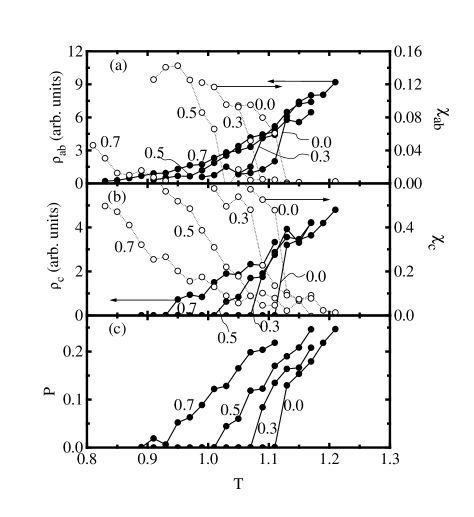
FIG. 1.: Resistivities $\rho_{ab},$ $\rho_{c},$ helicity modulus $\chi_{ab}$ and $\chi_{c},$ and percolation probability $P$ as a function of temperature for $\eta=1$ and different values of the disorder $D$ as indicated. Temperature is measured in units of the mean Josephson energy of the in-plane junctions. Magnetic field is $H=1/6$ quantum fluxes per plaquette.

Thermodynamical measurements agree with this picture. We calculated the helicity modulus parallel ($\chi_{c}$) and perpendicular ($\chi_{ab}$) to the field. Helicity modulus measures the influence on the energy of the system of a twist in the boundary conditions, and has to be different from zero to indicate superconducting coherence.[13] Open symbols in Fig. 1(a) and (b) show the values $\chi$ that correspond to the resistivity curves. In the case of the first order transition both $\chi_{c}$ and $\chi_{ab}$ have an abrupt drop at the melting temperature. For the highly disordered case $\chi_{ab}$ has a (smoother) decrease at $T_{i}$, whereas $\chi_{c}$ becomes nearly zero at $T_{p}$. The transition at $T_{p}$ is a percolation phase transition of the vortex structure as discussed in Refs. 14 and 12, that can be characterized by a percolation probability $P.$ The value of $P$ is the probability that a vortex path traversing the sample perpendicularly to the applied field exists. This value is zero below the transition and one above, with a transition zone that becomes narrower when $L_{ab}$ increases. The plot of $P$ vs temperature is shown in Fig. 1(c). We see that $\rho_{c}$ is different from (equal to) zero if $P$ is different from (equal to) zero.

FIG. 2.: Same as Fig. 1 but for a sample with anisotropy $\eta^{2}=20$. The values of $\chi_{c}$ for $D=0.3$ and $D=0.5$ are nearly zero within the considered temperature range.

In Fig. 2 we give the corresponding results for anisotropy $\eta^{2}=20$. The first order melting transition occurring for low disorder is similar to that observed for $\eta=1$, i.e., the inter-plane coherence is lost at the same temperature than the in-plane coherence. However, for higher values of disorder some differences occur: the inter-plane resistive transition occurs (to our numerical precision) at the same temperature as the in-plane transition $T_{i}$, but the percolation transition temperature $T_{p}$ (which for low anisotropy coincides with the resistive inter-plane transition) occurs for lower temperatures, i.e., $T_{p}<T_{i}$. This indicates that for high anisotropy, there is a temperature range $T_{p}<T<T_{i}$ for which percolation paths across the samples exist, however these path are not mobile (presumably because they are pinned to the planes, as $T<T_{i}$) and dissipation is not observed.[15]

From the above discussion on Figs. 1 and 2, the following picture emerges: at low disorder the vortex lattice melts through a first order phase transition. When disorder increases this transition breaks into two continuous ones, where in-plane and inter-plane coherence are lost at different temperatures $T_{i}$ and $T_{p}$. Whether $T_{i}$ is larger or lower than $T_{p}$ depends on the anisotropy of the system. For nearly isotropic samples $T_{i}$ is lower than $T_{p}$, and a disentangled vortex liquid phase exists for $T_{i}<T<T_{p}$. For highly anisotropic samples $T_{p}$ is lower than $T_{i}$ although dissipation along the c axis is observed only for $T>T_{i}$.

In Fig. 3 we show the numerical $D$-$\eta$ phase diagram as obtained from simulations. Stars indicate points where the melting transition is first order. Full circles are points where $T_{i}<T_{p}$, and hollow circles are points where $T_{p}<T_{i}$. This diagram shows the three different zones discussed above. The continuous line is a sketch of the frontiers between the different zones. In the next section we show that the main characteristics of this phase diagram can be derived from a simplified description of the vortex structure.

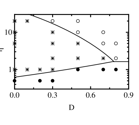
FIG. 3.: Disorder-anisotropy phase diagram as obtained from the simulations. Stars indicate points where the melting transition is first order. Full circles are points where $T_{i}<T_{p}$, and hollow circles are points where $T_{p}<T_{i}$. The continuous line is a sketch of the frontiers between the different zones.

III A simplified model

We saw in the previous section that a single first order transition is observed at low disorder, whereas two continuous ones are obtained in disordered samples. These features suggest that the system can be described as having in general two different transitions, but that in certain cases they can merge onto a single first order transition due to some kind of ‘interaction’. Here we show that this idea can be formulated more precisely by estimating the free energy of the system.

A Free energy functional

To make this estimation we will consider first a single clean plane. We suppose that the thermodynamics of that plane can be phenomenologically described by a quantity $\xi_{ab}$, which is a correlation length: for distances shorter than $\xi_{ab}$ the system has superconducting coherence, whereas this coherence is lost for distances larger than $\xi_{ab}$. The free energy functional ${\cal F}^{2D}$ of the plane has the form

$${\cal F}^{2D}=E^{2D}(\xi_{ab})-TS^{2D}(\xi_{ab})$$ (1)

(the thermodynamical free energy $F$ is obtained by minimizing with respect to $\xi_{ab}$). For a system of $L_{c}$ completely decoupled planes, we would have

$${\cal F}_{\eta\rightarrow\infty}^{3D}=L_{c}E^{2D}(\xi_{ab})-TL_{c}S^{2D}(\xi_{ab})$$ (2)

On the other hand, if the coupling between planes is infinite the vortices are rigid lines and we get

$${\cal F}_{\eta\rightarrow 0}^{3D}=-\left(\alpha/\eta^{2}\right)L_{c}+L_{c}E^{2D}(\xi_{ab})-TS^{2D}(\xi_{ab}).$$ (3)

Note that in this case the entropy term does not have the factor $L_{c}$ because giving the position of the vortices on one plane automatically determines the position of vortices in all other planes. The term $-\left(\alpha/\eta^{2}\right)L_{c}$ accounts for the energy gain due to the coupling of the planes, $\alpha$ being a numerical constant and $\eta$ the anisotropy parameter defined before. In an intermediate situation ($0<\eta<\infty$) the system can be thought as formed by $L_{c}/\xi_{c}$ layers ($\xi_{c}$ is a number that satisfies $1<\xi_{c}<L_{c}$). Within each layer the vortices are almost straight lines, whereas correlation is small between different layers. Within this picture the free energy of the system is

$${\cal F}^{3D}=-\left(\alpha/\eta^{2}\right)\left(L_{c}-L_{c}/\xi_{c}\right)+L_{c}E^{2D}(\xi_{ab})-T\left(L_{c}/\xi_{c}\right)S^{2D}(\xi_{ab}).$$ (4)

In the first term, $L_{c}-L_{c}/\xi_{c}$ is the number of sites along the c-direction at which the system gains an energy $\alpha/\eta^{2}$. The length $\xi_{c}$ is a correlation length along the c-direction. For distances shorter than $\xi_{c}$ the system possesses superconducting coherence, whereas this coherence is lost at distances greater than $\xi_{c}$.

The previous estimation of the free energy of the system is too crude. In particular, in the form given by Eq. (4), it leads to some unphysical results. We must modify Eq. (4) slightly in order to obtain the correct behavior in some limiting cases. However, we will keep a fundamental property of Eq. (4) and make the guess that the entropy can be written for the real system as

$$S=f(\xi_{c})S^{2D}(\xi_{ab}),$$ (5)

i.e., as a product of independent functions of $\xi_{c}$ and $\xi_{ab}$, with $f(\xi_{c})$ and $S^{2D}(\xi_{ab})$ two yet unknown functions. The basic assumption contained in (5) is the following: if the value of $\xi_{c}$ is kept fixed, then the system behaves as a two dimensional system with a renormalized temperature. Although this assumption cannot be fully justified a priori, it is a natural starting point, and gives sensible results as we will show soon.

We still have to add a term to the free energy which accounts for the effect of impurities. Impurities decrease the energy of the system when vortices pin to them. If pinning is uncorrelated the energy gain due to pinning becomes lower when the vortex positions are more correlated. So we add a term to the free energy that increases the energy of the system when $\xi_{ab}$ and $\xi_{c}$ increase. The most simple term of this type is of the form $D\xi_{ab}\xi_{c}$. Finally, the free energy functional of the system ${\cal F}\left(\xi_{ab},\xi_{c}\right)$ (dropping an irrelevant constant term) is

$${\cal F}\left(\xi_{ab},\xi_{c}\right)=\left(\alpha/\eta^{2}\right)L_{c}/\xi_{c}+L_{c}E^{2D}(\xi_{ab})-Tf(\xi_{c})S^{2D}(\xi_{ab})+D\xi_{ab}\xi_{c}.$$ (6)

The true expressions for the functions $f$, $E^{2D}$ and $S^{2D}$ are difficult to establish. However, it is not our aim to give a complete quantitative description of the free energy of the system but only a qualitative description of the phase diagram. We will only ask the functions $f$, $E^{2D}$ and $S^{2D}$ to reproduce some known limiting cases: if $\xi_{c}$ ($\xi_{ab}$) is kept fix we expect the value of $\xi_{ab}(T)$ ($\xi_{c}(T)$) obtained by minimizing ${\cal F}$, to be smoothly dependent on temperature. This corresponds to the absence of first order transitions in the dynamics of a single plane (a single vortex line).[16] However, when ${\cal F}$ is minimized with respect to both $\xi_{c}$ and $\xi_{ab}$ a  discontinuity in $\xi_{c}(T)$ and $\xi_{ab}(T)$ can appear, as we show below.

Just to give an example we use for the function $f$ the form $f=\gamma\ln\left(L_{c}/\xi_{c}\right)+1$. The term $\gamma\ln\left(L_{c}/\xi_{c}\right)$ ($\gamma$ is a numerical constant) is proportional to the entropy of a single (isolated) vortex line. The constant added assures that the two-dimensional limiting case is reobtained when $L_{c}=\xi_{c}$. In addition, we will take for the functions $E^{2D}$ and $S^{2D}$ the form $E^{2D}=L_{ab}/\xi_{ab}$ and $S^{2D}=\gamma\ln\left(L_{ab}/\xi_{ab}\right)+1$ , in such a way that we obtain a form for the free energy functional that is (unphysically!) symmetric (for $\alpha/\eta^{2}=1$) between ab- and c-directions. We have tested other forms of the functions $f$, $E^{2D}$ and $S^{2D}$ (giving the same limiting behavior discussed above) and found results qualitatively similar to those shown here.

We arrive to our final working expression of the free energy functional (we will measure $\xi_{ab}$ and $\xi_{c}$ in units of $L_{ab}$ and $L_{c}$, respectively, take $\alpha=1$ by rescaling $\eta,$ and also rescale $D$)

$${\cal F}\left(\xi_{ab},\xi_{c}\right)=1/\eta^{2}\xi_{c}+1/\xi_{ab}-T\left[\gamma\ln\left(1/\xi_{c}\right)+1\right]\left[\gamma\ln\left(1/\xi_{ab}\right)+1\right]+D\xi_{ab}\xi_{c}$$ (7)

The thermodynamical free energy $F$ is obtained by minimizing with respect to $\xi_{ab}$ and $\xi_{c}$:

$$F(T)=\min_{0\leq\xi_{ab}\leq 1}\min_{0\leq\xi_{c}\leq 1}{\cal F}\left(\xi_{ab},\xi_{c}\right)$$ (8)

We stress again we do not claim expression (7) is a good detailed description of the free energy of the system, but only a expression (which main characteristic is given by Eq. (5)), that will help us to understand different sectors of the $D$-$\eta$ phase diagram of high-$T_{c}$’s.

B Results

We present now the results obtained by minimizing the free energy functional given by expression (7). When doing this minimization we obtain the free energy $F$ and the lengths $\xi_{ab}$ and $\xi_{c}$ as a function of temperature. A first order transition is identified as a discontinuous derivative of $F$, or equivalently a jump in the values of $\xi_{ab}$ and $\xi_{c}$. When no jump in $\xi_{ab}$ and $\xi_{c}$ is obtained, the dependence of $\xi_{ab}$ and $\xi_{c}$ with temperature gives a clue on how the superconducting coherence is lost when raising temperature. However, in this case the identification of a phase transition is not simple, and we can only identify temperature ranges where coherence along c- or ab-directions is high or low.

Let us start with the case $D=0$ and $\eta=1$ (note that we are using a renormalized anisotropy parameter, so $\eta=1$ does not imply necessarily an isotropic system). In this case Eq. (7) is symmetric in $\xi_{ab}$ and $\xi_{c}$, and in fact the minima of ${\cal F}$ are on the line $\xi_{ab}=\xi_{c}\equiv\xi$, so in Fig. 4 we plot the function ${\cal F}(\xi,\xi)$ for different values of the temperature. We see that when $T\rightarrow 0$ the minimum free energy state corresponds to the maximum possible value of $\xi$, i.e., the system is in the ordered state. When temperature increases a first order transition to a disordered state occurs. This is also seen from the behavior of $\xi$ as a function of temperature, as depicted in Fig. 4(b). Thus we see that the coupling of two continuous transition (through the entropy term in (7)) can merge them onto a single one, which is first order. In fact, such sort of mechanism has been previously proposed to occur in other cases, such as two dimensional melting, in which the continuous dislocation-unbinding and disclination-unbinding transitions of the Kosterlitsz-Thouless-Halperin-Nelson-Young melting theory[17, 18] can collapse onto a first order melting transition.[18, 19]

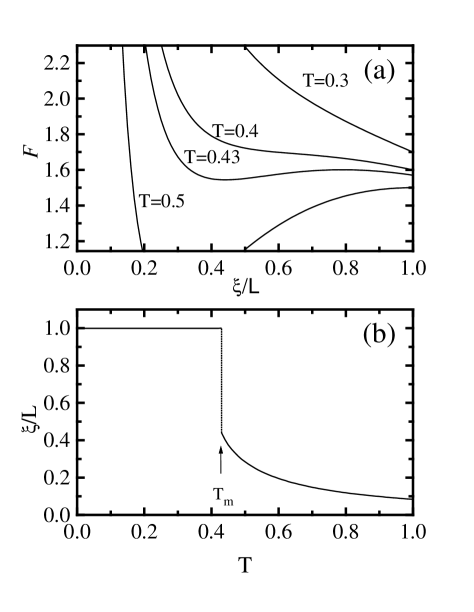
FIG. 4.: (a) Free energy functional as a function of correlation length $\xi$ for different temperatures with $D=0,$ and $\gamma=2$.(b) Correlation length as a function of temperature obtained as the minima of the curves in (a).

If disorder is present in the system it will tend to destroy the melting transition. In Fig. 5 we show results as those of Fig. 4 but for a value of $D=0.7$. As we see the jumps in $\xi_{ab}$ and $\xi_{c}$ have disappeared, indicating that the transition is not first order. If the anisotropy had been chosen different from one, then the temperature at which $\xi_{ab}$ and $\xi_{c}$ take a given value would have been different. Although we cannot characterize from our simplified model a phase transition when $\xi_{ab}$ and $\xi_{c}$ are continuous functions of temperature, it is tempting to say that if $\xi_{ab}$ ($\xi_{c}$) drops to zero at lower temperature than $\xi_{c}$ ($\xi_{ab}$), then we are in a sector of the phase diagram where $T_{i}<T_{p}$ ($T_{p}<T_{i}$). In this way we generate the phase diagram depicted in Fig. 6. As indicated, it is qualitatively similar to the one obtained from the numerical simulation, and it gives support a posteriori to the proposal of an entropy of the system of the form given by Eq. (5).

Some characteristics of this phase diagram can be analyzed in simple terms. For example, when $\eta\rightarrow\infty,$ the system is a set of decoupled planes, and no first order transition is obtained for any value of $D.$ When $\eta\rightarrow 0$ vortices are rigid lines and in fact effectively two-dimensional, so a first order transition is not obtained in this case either. This limiting cases give some insight on the form of the border between first-order and continuous transitions in Figs. 3 and 6. There is an optimum value of the anisotropy, at which the first order transition persists up to a highest value of disorder. This optimum value depends on the thickness of the sample. In fact, as we discussed in a previous work[12] the temperature $T_{p}$ logaritmically decreases when the thickness of the sample increases. This means that in Fig. 3 the border between the zones with $T_{i}>T_{p}$ and $T_{p}>T_{i}$ moves to lower values of $\eta$. It is thus likely that the optimum value of $\eta$ for the occurrence of the first order transition also decreases with sample thickness .

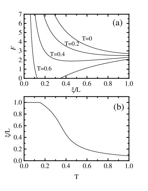
FIG. 5.: Same as Fig. 4 but with $D=0.7.$

IV Magnetic field dependence, and comparison with experiments

Having discussed the $D$-$\eta$ phase diagram for a fixed magnetic field $H$, we turn now to the discussion of the dependence on $H$. From the numerical point of view the direct approach would be to do simulations at different fields. However, as we discussed above, to reduce the magnetic field to other commensurate values would require exceedingly large computing time. Fortunately, there are arguments that suggest that a change of $H$ can be mapped onto a change of $D$ and $\eta$.

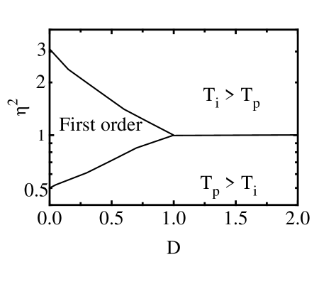
FIG. 6.: Disorder-anisotropy phase diagram as obtained by minimizing the free energy functional (see text for explanation).

The scaling combination between magnetic field and anisotropy has been given by Chen and Teitel.[20] We generalize here the argument to include the disorder parameter $D$. Our dimensionless temperature (measured in units of the mean Josephson energy of the in-plane junctions) can be only a function of the other dimensionless parameters of the system. These are $D$, $H$, and $\eta$. These parameters have different dependences on the coherence length $\xi_{0}$. If we identify the discretization parameter in the ab plane with a distance of the order of the coherence length $\xi_{0},$ then the critical current of the Josephson junctions along the c direction is proportional to $\xi_{0}^{2},$ so the anisotropy parameter $\eta$ behaves as $\xi_{0}^{-1}.$ On the other hand, our dimensionless magnetic field $H$ is given in terms of the real external magnetic field $H_{0}$ by the expression $H=H_{0}\xi_{0}^{2}/\phi_{0}$ ($\phi_{0}$ is the flux quantum). For the parameter $D$, we note that $D$ is proportional to the amplitude of the pinning potential. A vortex averages this random function on an area $\sim\xi_{0}^{2}.$ Considering the case of random (uncorrelated) pinning we find that $D$ depends on $\xi_{0}$ as $D\sim\xi_{0}^{-1}$. Since we are ignoring details of the vortex cores, we expect the $\xi_{0}$ dependence to cancel out, and our temperature transition to be only a function of the $\xi_{0}$-independent quantities $\eta^{2}H$ and $D^{2}H$.

We conclude that we can obtain the behavior of the system as a function of magnetic field from the results of Fig. 3 on lines with constant $D/\eta$. A sketch of the different possibilities is shown in Fig. 7. The general prediction from Fig. 3 is depicted in Fig. 7(a). The scales on the axis as well as the extent of the first order transition depend on the particular value of $D/\eta$. This general picture has to be modified at very low fields. In fact, a minimum crossover field[14] (given essentially as the field at which the vortex lattice parameter matches the thickness of the sample) exists, below which $T_{i}$ and $T_{p}$ are essentially the same (this is because in this case there are so few vortices in the sample that the transition is enterally due to thermally generated vortex loops). Different possibilities are depicted in Fig. 7 (b), and (c). They correspond to different ranges of values of $D/\eta$. Fig. 7(b) correspond to $D/\eta$ small, so Fig. 3 predicts $T_{p}<T_{i}$ at high fields, and a first order zone at intermediate and low fields. This phase diagram corresponds to that experimentally obtained for Bi₂Sr₂CaCu₂O,[21] which in fact has the largest value of $\eta,$ and even to the case of clean YBa₂Cu₃O₇,[22] which has a very low $D$. Fig. 7(c) shows the expected phase diagram for samples with a high value of $D/\eta$. At low fields $T_{i}$ is lower than $T_{p},$ whereas at high fields a cross to a zone with $T_{i}>T_{p}$ is possible. No first order zone is shown because a curve defined by a high value of $D/\eta$ in Fig. 3 do not pass through the first order zone. The low field part of this phase diagram corresponds to the one obtained for YBa₂Cu₃O₇ samples with defects.[23] The crossover to a case with $T_{i}<T_{p}$ has not been observed, presumably because of the high fields needed.

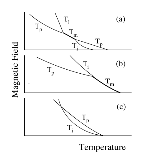
FIG. 7.: Qualitative sketch of the $H$-$T$ phase diagram for diferent calues of $D/\eta.$ (a) General form. (b) $D/\eta$ small. (c) $D/\eta$ high.

As we indicated above, when $T_{i}<T_{p}$ superconducting coherence is lost along the ab-plane at lower temperatures than along the c-axis. For $T_{i}<T<T_{p}$ finite resistance within the planes and zero resistance in the c-direction is observed. When $T_{i}>T_{p}$ and in the case that $T_{i}>T>T_{p}$ we potentially expect finite resistance in the c-direction and zero resistance within the planes. This has turned to be difficult to find, both experimentally [24] and in our simulations. The resistance seems rather to go to zero at the same temperature $T_{i}$ in all directions.[15] This is due to the fact that vortex paths crossing the sample for $T>T_{p}$ are pinned to the ab-planes as long as $T<T_{i}$, preventing their movement (and thus dissipation). However, it is worth noting that some other experimental measurements of coherence (AC magnetization) indicate[25] that in fact, c-axis coherence is lost at lower temperatures than in-plane coherence for the case of Bi₂Sr₂CaCu₂O.

The transitions observed in our simulations are of different character, and we want to discuss the point a bit further. The first order transition is the easiest to characterize numerically. Although we do not show all the results, we observed that when the resistivity has a jump other indicators point to a first order phase transition, among them the existence of hysteresis in the resistivity curves upon heating and cooling, and the fact that right at the transition temperature, the energy histogram of the system has two peaks, indicating two coexisting phases with an energy barrier separating them.[26, 4, 5] The continuous transitions are more difficult to characterize. The transition at $T_{i}$ is not a phase transition in our model. In fact, it is a crossover due to thermal deppining of rather independent vortices.[3, 12] However, in a real sample it may correspond to the vortex glass transition, depending on the strength of the disorder.[27] When $T_{p}>T_{i}$, we have previously characterized the transition at $T_{p}$ as a percolation phase transition of the vortex structure perpendicularly to the applied field.[12] In the thermodynamic limit for $L_{ab}$ ($L_{ab}\rightarrow\infty$) the system does not have any vortex line running perpendicularly to the applied field for $T<T_{p}$, whereas for $T>T_{p}$ these paths extend all over the ab plane with probability one. In References [14,12] we showed numerical evidence suggesting that this transition is a second order phase transition and gave its critical exponents as found from simulations.

V Summary and conclusions

In this paper we presented numerical evidence that supports an anisotropy-disorder phase diagram of the vortex structure of high-$T_{c}^{\prime}s$ with the following characteristics: For clean samples the vortex lattice melts through a first order phase transition for a wide range of anisotropies. When disorder is included the behavior of the system is strongly dependent of the anisotropy. For low anisotropies the in-plane coherence is lost at a temperature $T_{i}$ lower than the temperature $T_{p}$ at which inter-plane coherence is lost, and a zone of disentangled vortex lines is observed for $T_{i}<T<T_{p}$. For highly anisotropic samples the superconducting coherence as deduced from simulations of the resistivity is lost at the same temperature $T_{i}$ within the planes and perpendicularly to the planes. However, in this case the vortex structure percolates at a temperature $T_{p}$ well below $T_{i}$. In this case the system for $T_{p}<T<T_{i}$ is in an ‘entangled solid’ phase. These features are also obtained from an estimation of the free energy of the system which is mainly based on a proposal for the entropy of the system (Eq. (5)). We showed that the magnetic field-temperature behavior of the system can be deduced from results obtained from a fixed magnetic field provided the anisotropy and disorder present in the system are properly rescaled.

Our results present in a unified way, different characteristics of the vortex structure that had been previously found in partial studies. The analysis is in agreement with a variety of experiments performed on different materials with a broad range of parameters such as disorder, anisotropy and magnetic field. It could prove to be useful to find a more solid base of our proposal for the free energy of the system -that we showed is qualitative good- in order to obtain more detailed analytical results.

VI Acknowledgments

We thank helpful discussions with D. López, E. F. Righi and F. de la Cruz. E.A.J. acknowledges financial support by CONICET. C.A.B. is partially supported by CONICET.

REFERENCES

- [1] G. Blatter et al., Rev. Mod. Phys. 66, 1125 (1994).
- [2] D.Domínguez and J. V. José, Phys. Rev. B 48, 13717 (1993).
- [3] E. A. Jagla and C. A. Balseiro, Phys. Rev. B 52, 4494 (1995).
- [4] R. E. Hetzel, A. Sudbo, and D. A. Huse, Phys. Rev. Lett. 69, 518 (1992).
- [5] D. Domínguez, N. G. Jensen, and A. R. Bishop, Phys. Rev. Lett. 75, 4670 (1995).
- [6] H. Safar et al., Phys. Rev. Lett. 69, 824 (1992);W. K. Kwok et al., ibid. 72, 1092 (1994).
- [7] E. A. Jagla and C. A. Balseiro, to be published (Phys. Rev. Lett. Code LQ5742)
- [8] H. Pastoriza et al., Phys. Rev. Lett. 72, 2951 (1994).
- [9] E. Zeldov et al., Nature (London) 375, 373 (1995).
- [10] D. López et al., Phys. Rev. B 53, 8895 (1996).
- [11] D. López et al., Phys. Rev. Lett. 76, 4034 (1996).
- [12] E. A. Jagla and C. A. Balseiro, Phys. Rev. B 53, 15305 (1996).
- [13] M. E. Fisher, N. M. Barber, and D. Jasnow, Phys. Rev A 8, 1111 (1972); Y. H. Li and S. Teitel, Phys. Rev B 47, 359 (1993).
- [14] E. A. Jagla and C. A. Balseiro, Phys. Rev. B 53, 538 (1996).
- [15] In Ref. 12 we showed some results on anisotropic cubic lattices where a zone with and was observed. This dissipation is probably due to the movement of percolation paths lying entirely between two consecutive planes, and thus being unaffected by the pinning of the ab planes. We did not observe clearly the same effect on triangular lattices up to now.
- [16] A first order transition has been reported for a single plane (W. Yu, Ph D thesis, Ohio State University (1994), and also M. Franz and S. Teitel, Phys. Rev. B 51, 6551 (1995)). However, this transition is very weakly first order, and does not have inmediate relation with the one occurring on three-dimensional systems, where a strong first order transition is observed only if the thichness of the sample is higher than a critical value (See Reference [7] and also G. Carneiro, Phys. Rev. Lett. 75, 521 (1995)).
- [17] J. M. Kosterlitz and D. J. Thouless, L. Phys. C 6, 1181 (1973); A. P. Young, Phys. Rev. B 19, 1855 (1978).
- [18] B. I. Halperin and D. R. Nelson, Phys. Rev. Lett. 41, 121 (1978); D. R. Nelson and B. I. Halperin, Phys. Rev. B 19, 2457 (1978).
- [19] H. Kleinert, Gauge Fields in Condensed Matter, World Scientific, Singapore, 1989.
- [20] T. Chen and S. Teitel, unpublished.
- [21] F. de la Cruz et al., Physica B 197, 596 (1994).
- [22] D. López, E. F. Righi, S. Grigera, and F. de la Cruz, private communication.
- [23] F. de la Cruz, D. López, and G. Nieva, Philos. Mag. B 70, 773 (1994).
- [24] G. Briceño, M. Crommie and A. Zettl, Phys. Rev. Lett. 66 2164 (1991).
- [25] A. Arribere et al., Phys. Rev. B 48, 7486 (1993).
- [26] J. Lee and J. M. Kosterlitz, Phys. Rev. Lett. 65, 137 (1990).
- [27] M. I. J. Probert and A. I. M. Rae, Phys. Rev. Lett. 75, 1835 (1995).