Coherence-Incoherence Transition Between Fermi and Luttinger liquids

Abstract

We consider conditions for existence of fermionic quasiparticles in a strongly anisotropic quasi-one-dimensional metal. The adopted model is a model of chains of spin-1/2 Luttinger liquid coupled by small interchain hopping. It is shown that the Luttinger liquid becomes more stable with decrease of the lattice coordination number. It is also shown that with a significant spin-charge separation some Luttinger liquid features may persist in the Fermi liquid phase.

$Department~{}of~{}Physics,~{}University~{}of~{}Oxford,~{}1~{}Keble~{}Road,$
$Oxford,~{}OX1~{}3NP,~{}UK$

PACS numbers: 71.27.+a, 72.10.-d

There are quasi-one-dimensional materials which, despite being good conductors, display features which are considered as incompatible with the classical Fermi liquid description. It is suggested that the adequate description of these materials may be provided by the Luttinger liquid rather than the Fermi liquid theory. There are also materials like (TMTSF)₂PF₆ which being Fermi liquids under normal conditions show manifestly non-Fermi-liquid properties in a magnetic field [1], [2]. To give an adequate theoretical description of such systems one must understand a problem of stability of Luttinger liquid with respect to interchain hopping $t_{\perp}$. Despite that this problem has been addressed by many distinguished researches, there is still no consensus about the results. In this letter we argue that the existent results allow to establish sufficient conditions for stability of Luttinger liquids.

The most difficult aspect of the problem of stability of Luttinger liquid is that the interchain hopping simultaneously generates effects of different nature. Thus there are processes leading to creation of three dimensional Fermi surface and processes of multi-particle exchange leading to three dimensional phase transitions. Even if the Fermi surface is not formed, the interchain exchange will always destabilize the gapless Luttinger liquid fixed point and create a three dimensional ground state with a broken symmetry. In this and only this sense the interchain hopping is relevant. There is another question however, and it is whether the state above the transition temperature is a normal metal or something else. It was rightly pointed out by Anderson that the earmark of a Fermi liquid is a coherent transport in all directions (see also the discussions in Refs.[3],[4]). Meanwhile, in a one dimensional (or “confined”) Luttinger liquid state the Drude peak in optical conductivity exists only in the direction along the chains. Since the Drude peak in normal metals originates from existence of a well defined pole in the single electron Green’s functions which is absent in Luttinger liquid, we have to work out criteria for formation of such a pole.

To establish sufficient conditions for existence of the single particle pole one should make the phase transition temperature as low as possible. This can be achieved on a lattice with a large coordination number $D>>1$. This condition will allow us to ignore all feed back effects coming from electrons returning to the same chain and generating effective many-body exchange interactions leading to phase transitions at low temperatures. In order to minimize similarity between the Luttinger liquids on single chains and a Fermi liquid we shall consider a strong spin-charge separation $v_{s}/v_{c}<<1$.

Spin-1/2 Luttinger liquid can be described as a direct sum of charge and spin subsystems. The corresponding Hamiltonians describe free bosonic scalar fields with linear spectra: $\epsilon_{c,s}(q)=v_{c,s}|q|$. Except for the velocities $v_{c,s}$ the U(1)$\times$SU(2)-symmetric Luttinger Hamiltonian includes only one phenomenological parameter $K_{c}$ characterizing scaling dimensions in the charge sector. In our discussion we shall treat $K_{c}$ as an arbitrary parameter.

Taking into account only the diagrams which can be cut along a single hopping integral line as being leading ones in $1/D$, we get the following expression for the single electron Green’s function:

$$G(\omega,k,{\bf k})=[G_{0}^{-1}(\omega,k)-t_{\perp}({\bf k})]^{-1}$$ (1)

Here $G_{0}(\omega,k)$ is the Fourier transformation of the single chain Green’s function of the spin-1/2 Luttinger liquid, ${\bf k}$ represents transverse components of the wave vector and

$\displaystyle t_{\perp}({\bf k})=t_{\perp}\sum_{i=1}^{D}\cos({\bf k}{\bf b}_{i})$

with ${\bf b}_{i}$ being lattice vectors.

Eq.(1) was studied by Wen [5] who used various approximate expressions for $G_{0}(\omega,k)$. Wen demonstrated that at $T=0$ the pole appears when $\theta<1$ with

$\displaystyle\theta=(K_{c}+K_{c}^{-1}-2)/4$

Below we will partially repeat the Wen’s arguments and derive some new results. The retarded Green’s function has singularities near right and left Fermi points $k=\pm k_{\mbox{F}}$. In what follows we shall concentrate on the vicinity of the right Fermi point and introduce the wave vector $q=k-k_{\mbox{F}}$. The calculations of the single particle Green’s function of the Luttinger liquid carried out in Ref.[6] have established that at $T=0$ its imaginary part (the spectral function $\rho(\omega,q)$) is finite in the area represented on Fig. 1. In general we have

$$G_{0}^{(R)}[\omega,k=\pm(q+k_{\mbox{F}})]=\frac{|q/k_{\mbox{F}}|^{\theta}}{qv_{c}}\left[{\cal F}_{1}(\omega/v_{s}q)+\sin(\pi\theta/2){\cal F}_{2}(\omega/v_{c}q)\right]$$ (2)

The functions ${\cal F}_{i}$ can be extracted from the calculations of $G_{0}$ performed in Ref. [6]. For $q>0$ we have :

$${\cal F}_{1}(\omega/v_{s}q)=(v_{c}/v_{s})^{1+\theta}$$ (3)

$$\times\int_{0}^{v_{c}/v_{s}-1}\mbox{d}xx^{-1/2}(v_{c}/v_{s}-1-x)^{-1/2-\theta/2}(x+v_{c}/v_{s}+1)^{-\theta/2}(x+1+\omega/v_{s}q)^{-1+\theta}$$ (4)

$${\cal F}_{2}(\omega/v_{c}q)=\int_{0}^{\infty}\mbox{d}xx^{-\theta/2}(x+2)^{-1/2-\theta/2}(x+1+v_{s}/v_{c})^{-1/2}(x+1-\omega/v_{c}q)^{-1+\theta}$$ (5)

$$+\int_{0}^{\infty}\mbox{d}xx^{-1/2-\theta/2}(x+2)^{-\theta/2}(x+1-v_{s}/v_{c})^{-1/2}(x+1-\omega/v_{c}q)^{-1+\theta}$$ (6)

For $\theta<1$ these integrals converge at small $x$ and the answers are universal.

To study the Fermi surface formation, we need to know $G_{0}(\omega,q)$ at $\omega\rightarrow 0$. As follows from Eqs.(4, 6), in the area $-v_{c}q<\omega<v_{s}q$ ($q>0$) the Green’s function is purely real and can be expanded in powers of $\omega$. At $v_{s}/v_{c}<<1$ the leading contribution comes from the ${\cal F}_{1}$-term:

$${\cal F}_{1}(\omega/v_{s}q)=a-b\frac{\omega}{qv_{s}}+...$$ (7)

Substituting (7) into Eq.(1) we obtain the following expression for the dispersion law:

$$\epsilon(q,{\bf k})=\frac{a}{b}v_{s}\left[-q+av_{c}^{-1}t_{\perp}({\bf k})(|q|/k_{\mbox{F}})^{\theta}\right]$$ (8)

(mind that $q$ is counted from the old Fermi vector and therefore $q\neq 0$ at the new Fermi surface defined by $\epsilon(q_{\mbox{F}},{\bf k})=0$). So we see, that as it was originally found by Wen, the Fermi surface is formed at $\theta<1$ which corresponds to $3-2\sqrt{2}<K_{c}<3+2\sqrt{2}$. Large $K_{c}$ are probably unphysical, but small ones are certainly not. The widely quoted restriction $K_{c}>1/2$ is valid only for the Hubbard model. Small $K_{c}$’s are ubiquitous in CDW (charge density waves) materials (see, for example the review article [7], having in mind that in the literature on CDW $K_{c}$ is called $(m/m^{*})^{1/2}$). The reduction of $K_{c}$ comes mainly from retardation processes related to the electron-phonon interaction [8],[9]. The phonon-mediated interaction may also open a spin gap which would be undesirable for Luttinger liquid. However, the tendency to open a gap may be suppressed by a strong electron-electron repulsion which does not affect the retardation processes.

From Eqs.(1) and (8) we find the expressions for the new Fermi vector

$$\delta k_{\mbox{F}}=k_{\mbox{F}}\left[at_{\perp}({\bf k})/\epsilon_{\mbox{F}}\right]^{1/1-\theta}$$ (9)

(here and below $\epsilon_{\mbox{F}}=v_{c}k_{\mbox{F}}$) and the quasiparticle residue:

$$Z\approx\frac{v_{s}}{v_{c}}\frac{a^{2}}{b}\left[at_{\perp}({\bf k})/\epsilon_{\mbox{F}}\right]^{\theta/1-\theta}$$ (10)

As we shall see in a moment, the spin-charge separation plays an important role in the behavior of $Z$ providing an additional small parameter in the region $\theta<1/2$.

From Eq.(4) we find

$$a\approx(v_{c}/v_{s})^{1+\theta}\int_{0}^{v_{c}/v_{s}}\mbox{d}xx^{-1/2}(1+x)^{-1+\theta}(v_{c}/v_{s}-x)^{-1/2-\theta/2}(x+v_{c}/v_{s})^{-\theta/2}$$ (11)

The integral for $b$ is determined by $x\sim 1$ and can be calculated analytically:

$$b\approx(1-\theta)(v_{c}/v_{s})^{1/2}B(1/2,3/2-\theta)$$ (12)

where $B(x,y)$ is the beta function. The integral (11) has different areas of convergence depending on whether $\theta<1/2$ or $1/2<\theta<1$. In the former case it converges at $x\sim 1$:

$$a\approx(v_{c}/v_{s})^{1/2}B(1/2,1/2-\theta)$$ (13)

In the latter case the integral converges at large $x$ such that one can neglect a difference between $x$ and $x+1$ to obtain

$$a\approx(v_{c}/v_{s})^{\theta}B(\theta-1/2,1-\theta/2)F(\theta/2,\theta-1/2,1/2+\theta/2;-1)$$ (14)

where $F(a,b,c;x)$ is the hypergeometric function. Substituting Eqs.(13, 12, 14) into (10) we get

$$Z\sim\left(\frac{v_{s}}{v_{c}}\right)^{\gamma}\left[t_{\perp}({\bf k})/\epsilon_{\mbox{F}}\right]^{\theta/1-\theta}$$ (15)

where

$$\gamma=(1-2\theta)/2(1-\theta)>0,\>\>(\theta<1/2)$$ (16)

$$\gamma=(3-\theta)(1-2\theta)/2(1-\theta)<0\>\>(1>\theta>1/2)$$ (17)

Therefore we see that the exponent $\gamma$ changes its sign at $\theta=1/2$ which leads to a rather peculiar situation. Namely, at $\theta<1/2$ the single particle pole is formed, but its residue may be small even at moderately small $t_{\perp}/\epsilon_{\mbox{F}}$. This means that the Fermi liquid phase will retain many features of the Luttinger liquid (see Fig. 2). So for $\theta<1/2$ the spin-charge separation works in favor of the Luttinger liquid. For $\theta>1/2$ the situation is reversed: one needs a very high degree of one-dimensionality to get small $Z$. This apparently paradoxical behavior has a simple explanation. As follows from [6], at $\theta<1/2$ the single particle spectral function is singular at $\omega=v_{s}q$ and $\omega=v_{c}q$ (see Fig. 2 (a)). In the presence of hopping these singularities are smeared out, but the maxima still remain (Fig. 2(b)) and therefore, as we have said, many features of the system are still Luttinger-liquid-like. At $\theta>1/2$ these singularities disappear and the spectral function becomes featureless. Then when the pole is formed we will have a situation very much like in a conventional Fermi liquid: a featureless incoherent background and a sharp coherent pole.

Though all the above calculations have been carried out at zero temperature, we can make certain qualitative estimates for $T\neq 0$. According to the general principle of conformal field theory one can obtain expressions for finite temperature thermodynamic correlation functions from the $T=0$ expressions by replacing powers of $(\tau\pm\mbox{i}x/v)$ by the powers of $\sin\{\pi T(\tau\pm\mbox{i}x/v)]\}/\pi T$ ($\tau$ is the Matsubara time). After doing all necessary analytic continuations one obtains the following general expression which replaces Eq.(2) at finite $T$:

$$G_{0}^{(R)}[\omega,k=\pm(q+k_{\mbox{F}});T]=\frac{1}{T}(T/\epsilon_{\mbox{F}})^{\theta}{\cal F}(\omega/T,v_{s}q/T)$$ (18)

where ${\cal F}(x,y)$ is such that it is finite at $(x,y)\rightarrow 0$ and at $(|\omega,q|)>>T$ reproduces Eq.(2) (an explicit expression for ${\cal F}(x,y)$ will be published elsewhere). This consideration gives us an estimate of the temperature where a crossover from the Luttinger to Fermi liquid takes place:

$$T_{cross}\sim\epsilon_{\mbox{F}}\left[at_{\perp}({\bf k})/\epsilon_{\mbox{F}}\right]^{1/1-\theta}$$ (19)

Recently Clarke and Strong have also suggested [10] that the region $1/2<\theta<1$ is somewhat special. It is curious, that the incoherent transport also undergoes change at $\theta>1/2$ . Namely, (see Eq.(21)) the incoherent part of the transverse optical conductivity looses a characteristic maximum at $\omega=0$.

In the leading order in $t_{\perp}$ the real part of the transverse conductivity is given by the following expression (see, for example [5]):

$$\sigma_{\perp}(\omega)=\frac{e^{2}t^{2}_{\perp}}{2\pi^{2}\omega}\int\mbox{d}q\mbox{d}x[n(x)-n(\omega+x)]\rho(x,q;T)\rho(\omega+x,q;T)$$ (20)

where $n(x)$ is the Fermi distribution function and $\rho(x,q;T)$ is the finite temperature spectral function. Using the scaling form (18) we get

$$\sigma_{\perp}(\omega,T)=T^{-1+2\theta}{\cal S}(\omega/T)$$ (21)

This result holds for $T>>T_{cross}$ where one can neglect contributions to the conductivity coming from higher powers of $t_{\perp}$.

The transverse optical conductivity is relatively easy to measure and therefore one can use it to distinguish between Luttinger and Fermi liquid states. We argue that $\sigma_{\perp}(\omega,T)$ has different behavior as function of $\omega$ for $\theta>1/2$ and $\theta<1/2$. Indeed, as follows from Eq.(20), in both cases the conductivity is finite at $\omega=0$. At $\omega>>T$ it becomes independent on $T$: $\sigma_{\perp}(\omega>>T)\sim\omega^{-1+2\theta}$. This means that the function $S(x)$ is finite at $x=0$ and behaves as $x^{-1+2\theta}$ at $x>>1$. At $\theta<1/2$ this gives a peak at $\omega=0$ and for $\theta>1/2$ there is a minimum. In the latter case $\sigma_{\perp}(\omega,T)$ is qualitatively different from the coherent conductivity which has a Drude peak.

For $\theta<1/2$ it is more difficult because the transverse conductivity acquires a maximum at $\omega=0$ which may be confused with the Drude peak. In order to distinguish this incoherent maximum from the Drude peak one should measure the temperature dependence of its width $\Delta_{\omega}$. According to Eq.(21) $\Delta_{\omega}\sim T$; for a Fermi liquid we expect $\Delta_{\omega}\sim T^{2}$.

The Wen’s criterion $\theta>1$ is a sufficient one which is guaranteed to work at $D\rightarrow\infty$. Now we are going to argue that at small $D\sim 2$ the incoherent Luttinger liquid regime at finite temperatures may be realized at sufficiently weaker conditions. At finite $D$ there is a possibility that a three dimensional phase transition generated by the virtual interchain processes will happen at temperatures higher than those at which the single particle pole is formed. A probability of such outcome increases when $D$ decreases. The large $D$ approximation used in derivation of Eq.(1) becomes poor at small $D$, which opens an intriguing possibility that there is a critical value of $D$ below which a phase transition occurs at temperatures where the Fermi liquid pole is not yet developed. This may explain why the effective reduction of dimensionality in (TMTSF)₂PF₆ caused by a magnetic field has lead to non-Fermi-liquid effects reported in Ref.[1].

One may gain an insight from studying a case of two chains. It was pointed by Yakovenko [11] and Nersesyan et al. [12], who considered the case of spinless fermions, that under renormalization the hopping generates an effective interchain backscattering which (for two chains) may open a spectral gap. It is plausible that for an infinite number of chains instead of the gap one will get a phase transition. The corresponding renormalization group (RG) equations for fermions with spin were derived by Khveshchenko and Rice [13]. Below we shall analyze these equations following the approach of Ref.[11].

Without a loss of generality we may consider the case $K_{c}<1$. In this case the RG equations of Khveshchenko and Rice describe three possible regimes.

(i) Strong confinement regime. $K_{c}<3-2\sqrt{2}\approx 0.17$. This corresponds to the regime $\theta>1$.

(ii) Weak confinement regime. $3-2\sqrt{2}<K_{c}<\sqrt{5}-2\approx 0.24$. In this region, as we shall demonstrate in a moment, both single particle tunneling $t_{\perp}$ and dynamically generated interchain backscattering grow, but the latter interaction reaches the strong coupling regime first.

(iii) Band theory regime. $K_{c}>\sqrt{5}-2$. In this regime the best approach is to diagonalize the quadratic fermionic Hamiltonian first to obtain two split Fermi surfaces, and then take into account the interactions.

Let us consider the most interesting case (ii) which corresponds to

$$1/K_{c}-K_{c}>4$$ (22)

It can be shown that at these values of $K_{c}$ the effective exchange interaction is formed already at small distances. Condition (22) corresponds to rather small $K_{c}<0.24$, where the operators containing the dual fields $\Theta_{1,2}$ are strongly irrelevant. In this case we can simplify the RG equations Khveshchenko and Rice (see Eqs.(2. 6 - 21) in their paper) by retaining only the coupling constants $g_{1},g_{5}$ and $t_{\perp}$. Treating these coupling constants as small we shall also neglect renormalization of $K_{c,s}$ from their initial values $K_{c}<1,K_{s}=1$. Then we obtain the simplified version of the RG equations derived in Ref. [13], namely, we shall consider the case $K_{c}<1,K_{s}=1$ and neglect renormalization of these parameters. In this case Eqs.(2. 6 - 21) from Ref. [13] simplify:

$$\mbox{d}z/\mbox{d}l = \left[3-\frac{1}{2}(K_{c}+1/K_{c})\right]z,$$ (23)

$$\mbox{d}g/\mbox{d}l = (1-K_{c})g+(K_{c}-1/K_{c})z,$$ (24)

where $g=g_{1},g_{5}$ and $z=[t_{\perp}/\epsilon_{\mbox{F}}]^{2}$in the notations of Ref. [13]. We shall consider the case where the interchain exchange is absent in the bare Hamiltonian and generated dynamically in the process of renormalization. This corresponds to the following initial conditions: $g(0)=0$.

In this approximation we can solve Eq.(23):

$$z_{l}=z_{0}\exp\{[3-(K_{c}+1/K_{c})/2]l\}$$ (25)

Substituting this into Eq.(24) and taking into account the initial condition $g(0)=0$ we get

$$g_{l}=-\frac{z_{0}(1/K_{c}-K_{c})}{1/K_{c}-K_{c}-4}\left\{1-\exp[-l(1/K_{c}-K_{c}-4)/2]\right\}\exp[(1-K_{c})l]$$ (26)

Let us suppose that $(K_{c}^{-1}-K_{c}-4)$ is not very small. Then $g_{l}$ becomes of order of one at

$$l^{*}\approx-\frac{1}{(1-K_{c})}\ln z_{0}$$ (27)

Substituting it into Eq.(25) we get

$$z(l^{*})\approx z_{0}^{\frac{K_{c}^{-1}-K_{c}-4}{2(1-K_{c})}}$$ (28)

Since the exponent is positive and $z_{0}<<1$, this means that at the point where the effective exchange is already strong and presumably opens a spectral gap, the single particle tunneling is still weak.

As we have said, it is plausible that the gap opening in the two chain model is a precursor of a phase transition in the two dimensional array of chains. Thus we conclude that for $D=2$ the conditions for existence of Luttinger liquid are relaxed: instead of having Luttinger liquid phase at $K_{c}<0.17$ one may have it (at finite temperatures, of course) already at $K_{c}<0.24$. A presence of bare interchain interactions (the Coulomb interaction, for instance) will further relax the condition on $K_{c}$.

I am grateful to L. Degiorgi for information about his experiments, to N. Andrei, A. G. Green and V. Yakovenko for valuable discussions and constructive criticism. I am greatly indebted to K. Schönhammer who pointed out the mistake in the first version of the paper.

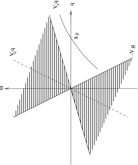
FIG. 1.: The shaded region is the region of $(\omega,q)$ plane where $\Im mG_{0}^{(R)}$ for the single chain does not vanish. The solid line shows the dispersion law of the coherent fermion excitation near the right Fermi point.

FIG. 2.: (a) The spectral function for the spin-1/2 Luttinger liquid at $\theta<1/2$, $q>0$, (b) the same in the presence of the quasiparticle peak.

REFERENCES

- [1] G. M. Danner and P. M. Chaikin, Phys. Rev. Lett. 75, 4690 (1995).
- [2] M. Dressel, A. Schwartz, G. Grüner and L. Degiorgi, Phys. Rev. Lett. 77, 398 (1996).
- [3] D. G. Clarke, S. P. Strong and P. W. Anderson, Phys. Rev. Lett. 72, 3218 (1994);
- [4] D. G. Clarke and S. P. Strong, Ferroelectrics 177, 1 (1996).
- [5] X. G. Wen, Phys. Rev. B42, 6623 (1990).
- [6] V. Meden and K. Schönhammer, Phys. Rev. B 46, 15 753 (1992); J. Voit, Phys. Rev. B 47, 6740 (1993); Y. Ren and P. W. Anderson, Phys. Rev. B 48, 16 662 (1993).
- [7] G. Grüner, Rev. Mod. Phys. 60, 1129 (1988).
- [8] S. A. Brazovskii and I. E. Dzyaloshinskii, Sov. Phys. - JETP, 44, 1233 (1976).
- [9] H. Fukuyama, J. Phys. Soc. Jpn. 43, 513 (1976); H. Fukuyama and P. A. Lee, Phys. Rev. B17, 535 (1978).
- [10] D. G. Clarke and S. P. Strong, cond-mat/9607141.
- [11] V.M.Yakovenko, JETP Lett. 56, 5101 (1992).
- [12] A. A. Nersesyan, A. Luther and F. V. Kusmartsev, Phys.Lett. A 176, 363 (1993).
- [13] D. V. Khveshchenko and T. M. Rice, Phys. Rev. B50, 252 (1994).