Two point-contact interferometer for quantum Hall systems

Abstract

We propose a device, consisting of a Hall bar with two weak barriers, that can be used to study quantum interference effects in a strongly correlated system. We show how the device provides a way of measuring the fractional charge and fractional statistics of quasiparticles in the quantum Hall effect through an anomalous Aharanov-Bohm period. We discuss how this disentangling of the charge and statistics can be accomplished by measurements at fixed filling factor and at fixed density. We also discuss a another type of interference effect that occurs in the nonlinear regime as the source-drain voltage is varied. The period of these oscillations can also be used to measure the fractional charge, and details of the oscillations patterns, in particular the position of the nodes, can be used to distinguish between Fermi-liquid and Luttinger-liquid behavior. We illustrate these ideas by computing the conductance of the device in the framework of edge state theory and use it to estimate parameters for the experimental realization of this device.

PACS: 73.23.-b, 71.10.Pm, 73.40.Hm, 73.40.Gk

I Introduction

A considerable amount of work on electronic systems in recent years has focused on two distinct sets of problems: the effects of quantum interference on the behavior of mesoscopic systems and those of strong correlations in low dimensional systems. Most of the canonical work on the former [1] has involved single electron physics while work on strongly correlated electrons has, by definition, been concerned with the effects of inter-electron interactions. Recent advances in semiconductor device fabrication have led to a convergence of these streams of work, in that it is now possible to conduct experiments that test quantum interference in strongly interacting systems of electrons.

The work reported here takes advantage of this convergence. Our principal motivation is the physics of the fractional quantum Hall (FQH) states, which exhibit some of the most striking effects of strong electronic correlations. These are perhaps most evident in the unusual quantum numbers of FQH quasiparticles: they are fractionally charged [2], obey fractional statistics [3, 4] and couple to curvature with a fractional spin [5, 6, 7]. These correlations also lead to a novel dynamics at the edges of FQH systems which is that of one dimensional chiral Luttinger liquids [8].

Our chief purpose in this paper is to describe and analyze a device, the two point-contact interferometer, that would allow direct observation of the fractional charge and statistics of the quasiparticles as well as allow tests of the chiral Luttinger liquid behavior of the edges; the former function is largely independent of and more robust than the latter. This device has remarkably rich interferometric possibilties; it exhibits conductance oscillations with varying magnetic field and also with varying amplitude of the voltage across it.

The paper is organized as follows. In the balance of the introduction we discuss some related work. In Section II we describe the interferometer and give a qualitative discussion of its physics in a largely model independent way. In Section III we introduce a model, defined in terms of edge state theory, that allows explicit calculations of the conductance of the device. We treat the model within perturbation theory and solve for the transmission current which displays oscillations with both magnetic field and voltage. In Section IV we consider the exactly solvable case in which the edge states are chiral Fermi liquids. This is the case for edge states of an integer filling factor state ($\nu=1$), and helps provide an intuitive understanding of the voltage interference patterns for general $\nu$. Finite temperature effects are treated in Section V, where we show how the oscillations are washed out as the temperature is raised. In Section VI, we give numerical estimates for the sizes of the parameters at which the Aharonov-Bohm and voltage oscillations occur. The appendix contains the details of the perturbative calculation of the transmission current.

A Related Work

The direct observation of fractional quantum numbers in FQH systems has long been of interest. Pokrovsky and Kivelson [9] suggested ways in which the fractional charge could be detected through a fractional Aharanov-Bohm period. This has been elaborated further in the work of Kivelson [10] and of Pokrovsky and Pryadko [11]. Strong evidence of such oscillations was found in the experiment of Simmons et al [12], who measured conductance oscillations on the edges of various QH plateaux. However it has not been clear what microscopic details of the transport in that region led to these oscillations. It is our current belief that most likely their sample fortuitously realized a version of the interferometer discussed here. Recent experiments involving tunneling across an antidot in a FQH sample [13, 14], have provided convincing evidence for a fractional local charge [15] that couples to the electrochemical potential. Finally, Kane and Fisher [16] and Chamon, Freed and Wen [17, 18, 19] have suggested that measurements of the noise for tunneling currents between the edges of a FQH system, i.e. in a single point-contact device, could be used to detect the fractional charge; calculations of the zero frequency noise for the exactly integrable model have been carried out by Fendley et al. [20].

The detection of fractional statistics remains unaddressed by experiments to date. The theoretical basis for such a detection was first discussed by Kivelson [10] and an intriguing proposal involving flux periodicities for hierarchy droplets inside FQH systems has been proposed by Jain, Thouless and Kivelson[21]. The observation of the fractional spin seems quite difficult and still awaits a concrete scenario for an experiment.

Finally, our concrete discussion of the physics of the interferometer in the framework of edge state theory [22] expands the scope of the work on tunneling in chiral Luttinger liquids by Wen [17], and the work on resonant impurity tunneling in Luttinger liquids by Kane and Fisher [23]. A very recent paper by Geller et al [24] discusses resonant tunneling through anti-dots and although theirs is a distinct geometry, and they consider only electron tunneling, their treatment is similar to ours.

II Device Description and Qualitative Discussion

The device we are proposing consists of three components, as illustrated in Figure 1. The first and primary component is a narrow quantum Hall bar with two tunable constrictions, or point-contacts, whose separation is less than a phase coherence length at low temperatures. The second component is a back gate that allows the electron density in the Hall bar to be varied uniformly. The third component is another gate (e.g. an air bridge) that would allow the center of the region defined by the two point-contacts to be selectively depleted by the application of a voltage. Estimates for the dimensions of the device, which seem entirely feasible with existing fabrication techniques, are discussed in Section VI; here we note that these require that the point contacts be a few microns apart for operating temperatures of 100mK and below and that the electron gas be about 1000$\AA$ or less from the point-contacts and the central gate. The back gate is not required to be particularly close to the electron gas.

The physics of this device is that of a quantum version of the Fabry-Perot interferometer[26]. However, our interferometer differs from the standard non-interacting one in that the scattering particles cannot be assumed to be independent because of the strong correlations. At values of the magnetic field where the electrons in the bulk of the device are deep in a QH phase, the low energy excitations, or quasiparticles, lie on the edges of the bar. At the constrictions, they can tunnel from one edge to another and the resulting tunneling current will cause the Hall conductance to deviate from its quantized value, as in the case for a single point-contact. However, having two tunneling sites results in phase sensitivity of the tunneling current; tunneling events taking place at one of the contacts will interfere with those occuring at the other.

These interference effects can be modulated in three distinct ways: The first involves changing the magnetic field and leads to what we shall call Aharanov-Bohm (AB) oscillations for obvious reasons. The second involves changing the number of quasiparticles enclosed by the interfering orbitals and leads to (fractional) statistical oscillations. The third involves varying the source-drain voltage and leads to what we shall call a novel set of “Fabry-Perot” oscillations. In the following we will show how these various effects can be disentangled to provide a means of measuring both the fractional charge and fractional statistics of the quasiparticles as well as to probe the non-Fermi (Luttinger) liquid behavior of the edges of FQH states.

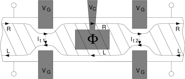
FIG. 1.: Two point-contact interferometer. Two gates are placed a distance $a$ apart. The gate voltages are adjusted so as to bring the edges of a FQH state with filling fraction $\nu$ close together, but not pinch the constriction. In this way, quasiparticles carrying fractional charge and statistics can tunnel from one edge to the other. A magnetic flux $\Phi$ can be inserted in the region between the point-contacts that is bounded by the edge states. A central gate allows the charge in the region to be selectively depleted. The transmitted current (the Hall current $I_{H}=\nu e^{2}/h$ minus the tunneling current $I^{1}_{t}+I_{t}^{2}$) oscillates as a function of the inserted flux, the voltage difference between the edges and the voltage of the central gate. An overall back gate on the device allows magnetic field sweeps at constant filling factor.

We would like to emphasize that we will always be interested in the limit where the barriers are weak, so that the constrictions are far from being pinched off, as in Figure 1. (The opposite limit, where the two point-contacts are near pinch off, is similar to tunneling through a quantum dot, except that for our geometry the central island would be larger. It can be analyzed using methods similar to those in this paper, but we will not address it here.) The chief advantage of this restriction is that we stay far from the regime near pinch off where, experimentally, poorly understood resonances arise already for a single point-contact [27]. Consequently, we expect that the only resonances are the ones explicitly created by the two point-contact geometry and the resulting energy and field scales for these are set by the parameters of the device and can be chosen to lie in an observable range. (Given the lack of understanding of the near pinch-off resonances, it is hard to say theoretically whether they are absent for weak barriers; however, experiments involving antidot resonances [13, 14] do strongly suggest this.) Further, it becomes possible to probe the internal structure of the resonance, i.e. its intermediate energy behavior, without detailed microscopic knowledge. Another restriction on our analysis is that we consider only the primary Hall states, i.e. $\nu=1/m$ with $m$ odd, where there is only one branch of edge excitations and life is somewhat simpler; the extension to their descendant states does not pose any conceptual problems.

A Aharonov-Bohm and fractional statistics oscillations

We will first discuss the interference effects which occur when the magnetic field is varied. Consider the transmission amplitude for quasiparticles propagating along the right edge. As they can tunnel to the left edge at the two constrictions in Fig. 1, the amplitude will involve a sum over paths that encircle the area $A$ enclosed by the edges and the constrictions any number of times. As a result, they pick up an AB phase proportional to the flux $\Phi$ through this area. Naively, this phase is given by $2\pi e^{*}BA/(hc)$, where $e^{*}$ is the charge of the quasiparticle. It is convenient to define an effective flux quantum by $\Phi^{*}={e\over e^{*}}\Phi_{0}$, where the usual flux quantum is given by $\Phi_{0}=hc/e$. Then, in terms of this effective flux quantum, we would expect that as the magnetic flux is varied, the current and other properties of the system would undergo oscillations with period $\Delta B^{*}=\Phi^{*}/A$, and thus measurements of these oscillations would provide a means of measuring the fractional charge.

However, this conclusion is too naive. The quasiparticles derive their properties from the parent liquid which is the relevant “vacuum” and only when the vacuum is invariant can we expect to use arguments based solely on their AB phases. Indeed, if the extra flux added is dynamically localized in the interior of the fluid this would effectively create a multiply connected geometry where gauge invariance for the constituent electrons implies a flux periodicity of $\Delta B=\Phi_{0}/A$. As this is smaller than the quasiparticle period $\Delta B^{*}$, this would exclude oscillations with the latter periodicity. We should emphasize that this is a dynamical possibility, there are no general, non-trivial consequences of gauge invariance for the geometry at issue here. At any rate, it is clear that we need to be careful about considering changes in the bulk of the fluid as the flux is varied. To this end we distinguish between two cases.

i)Field sweeps at fixed particle number: In this case, as we just observed, we expect to observe conductance oscillations with period $\Phi_{0}/A$. This can happen in one of two ways depending upon the detailed electrostatics of the central region. If, as the magnetic field is raised, the QH fluid in the central region shrinks uniformly in order to keep the filling fraction constant, then its area decreases by just the right amount to leave the flux through the whole droplet unchanged. Consequently, there are no oscillations as the magnetic field is varied and the period is trivially $\Phi_{0}/A$. If, instead, the electrostatics prefers otherwise and the self-consistent potential has a maximum in the interior, quasiholes will be created there as the magnetic field is increased—one quasihole for each flux quantum. The phase picked up by a quasiparticle encircling the central region is now the sum of the fractional AB phase and the phase $-\theta^{*}=-2\pi/m$ due to its (fractional) statistical interaction with the central quasihole and precisely restores the periodicity to $\Delta B$.

ii)Field sweeps at fixed filling factor: One obtains quite different results if the field is swept at fixed filling factor. In this case the quasiparticles see an invariant vacuum (in other words, the electron density is changed so that quasiholes are not formed in the bulk of the droplet). The resulting periodicity is then $\Delta B^{*}$. The observation of conductance oscillations with such a fractional AB period would constitute a measurement of a fractional AB charge for the quasiparticles. Experimentally, keeping the filling factor constant requires changing the number of particles along with the field which is why the device requires a back gate. Also, preventing the formation of quasiholes in the central region requires that net fractional charge be added to the this area, which is only possible if the contacts are not pinched off.

Having discussed the observation of fractional charge we now turn to the observation of fractional statistics. We first note that the comparison between the periodicity $\Delta B$ when the number density $n$ of electrons is held constant and the periodicity $\Delta B^{*}$ when the filling fraction $\nu$ is held constant, implicitly verifies the fractional statistics of the quasiparticles and quasiholes, because in one case the period is due to the combined effects of the Aharonov-Bohm phase and fractional statistics, and in the second it is due only to the Aharonov-Bohm phase.

To more directly see the effect of the fractional statistics, we need to consider oscillations that arise from having varying numbers of quasiparticles in the central region. If $N$ quasiholes are present, then the interference phase is modified to $2\pi(BA/\Phi^{*}-N/m)$. It is clear then that it is neccessary to add $m$ quasiparticles before the interference condition is restored. To this end one can imagine using the central gate to deplete the central region in steps of charge $1/m$ which would then lead to conductance oscillations with a period of $m$ steps. A better strategy, which requires less control over the electrostatics, is to create some unknown number of quasiholes in the central region and then look for a shifted fractional AB pattern at fixed filling factor, as in the charge measurement. Except when an integer multiple of $m$ quasiholes are present, there will be a shift in this pattern and the observation of $m-1$ distinct shifts will be a direct signature of the statistical interaction between the quasiparticles. For example, at $\nu=1/3$, there will be two shifted patterns with shifts of $(1/3)\Delta B^{*}$ and $(2/3)\Delta B^{*}$.

B Fabry-Perot oscillations due to finite source-drain voltages

The third modulation of the interference appears when varying the source-drain voltage $V$, and again leads to oscillations in the conductance. The origin of these oscillations is most transparent for $\nu=1$, where single-particle considerations suffice; this is detailed in Section IV. In brief, the conductance at finite $V$ is determined by the transmission of electrons in a range of energies $\Delta E=eV$ while the transmission itself oscillates with energy. Consequently, the integrated transmission, and hence the conductance itself, oscillates with the source-drain voltage, albeit with an envelope that decreases as $1/V$.

An interesting perspective is afforded by thinking in analogy to the classical wave analysis of the Fabry-Perot interferometer, i.e. a device with two parallel partially transmitting barriers; as we shall see in the edge state analysis of the device, it is conceptually exact and allows a unified treatment of the fractional fillings as well. Evidently, the combination $\omega_{\rm osc}=2\pi/\tau$, the inverse time for edge waves (and hence the quasiparticles) to travel from one point-contact to the other, is the characteristic frequency of the device and will set the scale for the oscillations in its transmission due to multiple reflections within it. The source-drain voltage defines a second frequency scale, the Josephson frequency $\omega_{J}=e^{*}V/\hbar$, where $e^{*}$ is the fractional charge of the quasiparticles living on the edges; this is the bandwidth of the waves incident on the interferometer. It follows then that the transmission will be a function of the ratio $\omega_{J}/\omega_{\rm osc}$ as well as of the reflection/transmission coefficients at the point-contacts which are determined by the quasiparticle tunneling amplitudes at them.

Because the right-moving and left-moving waves lie on the edge of a QH droplet, there is a second perspective that is very illuminating. (This picture, however, is not as general as the actual calculation of the voltage oscillations, since the calculation does not explicitly require the left- and right-moving edges to enclose any amount of flux; it would also be valid for a 1D wire if the modes were to have differing chemical potentials.) In this picture, the Aharonov-Bohm phase is responsible for the oscillations in the transmission as the energy is varied because the different energies lead to different areas enclosed by the interfering orbits. More specifically, an increase in energy of $\delta E$ corresponds to a change in the momentum of the quasiparticles given by $\delta k=\nu\delta E/(\hbar v)$, where $v$ is the velocity of the edge modes [28]. The momentum at the edge is related to the area of the droplet $A$ and its perimeter $2a$ by $k=\nu A/(l^{2}2a)$, where $l$ is the magnetic length, so that an increase of $\delta E$ in energy results in an increase in area of $\delta A=2l^{2}a\delta E/(\hbar\nu v)$. The extra flux enclosed then gives a change in phase of $2\pi\delta\Phi/\Phi_{0}^{*}=2a\delta E/\hbar v=4\pi\delta E/\hbar\omega_{\rm osc}$. As a result, as the energy is varied, the transmission oscillates with a period set by $\omega_{\rm osc}$ [29].

Three conclusions follow from this description. First, we recover the result that the net transmission has a component that oscillates with the source-drain voltage. Second, we find that there are two distinct regimes as a function of $\omega_{J}/\omega_{\rm osc}$. For small values of this ratio the device is probed at low frequencies and hence at a long length scale where the coherence between the two barriers is important. In this regime the phase difference between the reflection/transmission coeffecients at the barriers governs the transmission. Because this phase difference is determined by the AB phase, the AB oscillations discussed in the previous section will occur. At large values of the ratio, the barriers enter independently and the AB oscillations are washed out. The third and most interesting conclusion is that even for intermediate values of the ratio there are special points where the AB oscillations disappear. Again, the origin of this disappearance is most transparent for $\nu=1$: the nodes occur whenever the bandwidth is equivalent to a phase difference of an integer multiple of $2\pi$ across it. In such cases the phase shift between the barriers is immaterial; essentially, one is integrating the interference pattern over an integral number of periods, so the oscillations cancel.

The detailed analysis in Section III, where we consider the case of general $\nu$, bears out the same qualitative feature that there are special values of $V$ where the AB oscillations disappear. However, the location of these nodes is modified in a very interesting way which depends sensitively upon the nature of correlations in the edges. If the edge dynamics are of the Fermi liquid variety, as should be the case at $\nu=1$, our naive assertions are correct. However, if the edges are Luttinger liquids then the locations of the nodes are given by the zeros of Bessel functions which depend on $\omega_{J}/\omega_{\rm osc}$, and the type of Bessel function depends on the Luttinger liquid exponent $g$. The nodes occur for $\omega_{J}/\omega_{\rm osc}\approx(n+\xi_{g})/2$, $n=0,1,\dots$, with the $g$ dependent shift $\xi_{g}=(1+g)/2$. For quasiparticle tunneling, where $g=\nu$, this shift is not an integer, and can, in principle, be used to measure $g$! (Given an independent measurement of $v$, this also allows a measurement of $e^{*}$.) Thus it follows that the interferometer can also be used to distinguish between Fermi liquid (with $g=1$) and Luttinger liquid behavior at the edges of FQH systems.

In the qualitative discussions of the Aharonov-Bohm and Fabry-Perot oscillations above, we have considered the zero temperature case for simplicity. The effects of finite temperature, particularly the suppression of quantum interference, are treated quantitatively in Section V.

III Tunneling between edge states in the double point-contact geometry

We will now study the interferometer in the framework of edge states in the quantum Hall effect, which is better cast in the bosonic language (for a thorough review, see Ref. [22]). Our starting point for studying tunneling in a double point-contact geometry is the Lagrangian density

$${\cal L}=\frac{1}{8\pi}[(\partial_{t}\phi)^{2}-v^{2}(\partial_{x}\phi)^{2}]\ -\ \sum_{i=1,2}\Gamma_{i}\ e^{-i\omega_{J}t}\ \delta(x-x_{i})\ e^{i\sqrt{g}\phi(t,x_{i})}+H.c.\ \ ,$$ (1)

with the quantization condition $[\phi(t,x),\partial_{t}\phi(t,y)]=4\pi i\delta(x-y)$. (We use this normalization of $\phi$ because it gives an especially simple expression for the dimensions of the tunneling operators in terms of $g$. To translate to the conventional normalization of a 1D electron gas or the sine-Gordon model, $\phi$ must be replaced by $\phi/(2\sqrt{\pi})$.) The voltage difference between the two edges of the QH liquid determines the Josephson frequency $\omega_{J}\equiv e^{*}V/\hbar$, with $e^{*}=e$ for electron tunneling and $e^{*}=e/m$ for quasiparticle tunneling. In the following we will set the edge velocity $v=1$. The two point-contacts are located at $x_{1}$ and $x_{2}$, and their tunneling amplitudes are $\Gamma_{1}$ and $\Gamma_{2}$, respectively [30].

The first term in the Lagrangian, when considered alone, describes the dynamics of a free boson field $\phi=\phi_{R}+\phi_{L}$, which can be decomposed into its chiral components $\phi_{R,L}$. These components describe right and left moving excitations along the edges of FQH states. Charge density operators can be defined in terms of the $\phi_{R,L}$ through $\rho_{R,L}=e\frac{\sqrt{\nu}}{2\pi}\partial_{x}\phi_{R,L}$.

The second term in the Lagrangian comes from the tunneling between the edges. The tunneling operators can be written as $\Psi^{\dagger}_{L}\Psi_{R}$ and $\Psi^{\dagger}_{R}\Psi_{L}$. Right and left moving electron and quasiparticle operators on the edges of a FQH liquid are given by $\Psi_{R,L}(t,x)\propto e^{\pm i\sqrt{g}\phi_{R,L}(t,x)}\ e^{\pm ik_{F}x}$, where $g$ is related to the FQH bulk state. For example, for a Laughlin state with filling fraction $\nu=1/m$ we have $g=m$ for electrons and $g=1/m$ for quasiparticles carrying fractional charge $e/m$. One can verify that $[\rho_{R,L}(t,x)\ ,\ \Psi^{\dagger}_{R,L}(t,y)]=e\sqrt{\nu g}\ \Psi^{\dagger}_{R,L}(t,y)\delta(x-y)$, so that indeed the cases $g=\nu^{-1}$ and $g=\nu$ correspond to the electron ($e^{*}=e$) and quasiparticle ($e^{*}=\nu e$) creation operators, respectively.

The flux $\Phi$ in the area enclosed by the edge branches between the two point-contacts is taken into account by the phase of the tunneling amplitudes, $\Gamma_{i}$, in Equation (1) . This phase comes from the quasiparticle’s momentum $k_{f}$ in the definition of $\psi_{R,L}$. From this definition, the tunneling operator $\psi_{L}^{\dagger}(x)\psi_{R}(x)$ has the phase $e^{2ik_{f}x}$, where $2k_{f}$ is equal to the momentum difference between the right-moving edge and the left-moving edge. The momentum difference $2k_{fe}$ between electrons on the two edges is directly related to the perimeter $L$ and area $A$ of the QH liquid confined between the two point-contacts. It is given by $k_{fe}L=2\pi BA/\Phi_{0}$. If the distance between the two edges at each of the point-contacts is much smaller than the distance $a$ along an edge between the two contacts, then the perimeter can be set equal to $2a$. For $\nu=1/m$, with $m$ an integer, the momentum of the quasiparticles is then given by $2k_{f}=\nu 2k_{fe}=2\pi\Phi/(\Phi^{*}a)$. Because $\Gamma_{1}$ is the amplitude for tunneling at $x=-a/2$, it has the phase $e^{i2\pi\Phi/(2\Phi^{*})}$, and similarly $\Gamma_{2}$ has the phase $e^{-i2\pi\Phi/(2\Phi^{*})}$. Thus, the flux can be introduced in Equation (1) by taking $\Gamma_{1,2}={\bar{\Gamma}}_{1,2}e^{\pm i2\pi\Phi/(2\Phi^{*})}$, where ${\bar{\Gamma}}_{1,2}$ are couplings which do not include the phase due to the magnetic flux. Combining these together, we find that a quasiparticle that circles the area between the two constrictions once (by tunneling from the left-moving edge to the right-moving edge at $x=-a/2$ and tunneling back to the left-moving edge at $x=a/2$) picks up the amplitude $\Gamma_{1}^{*}\Gamma_{2}={\bar{\Gamma}}_{1}^{*}{\bar{\Gamma}}_{2}e^{-2\pi i\Phi/\Phi^{*}}$, so that the phase of the tunneling amplitudes determines the Aharonov-Bohm phase.

The form of the phases appearing in the amplitudes $\Gamma_{1}$ and $\Gamma_{2}$ can also be viewed as coming from the interaction of the bosonic edge states $\phi$ with the electric and magnetic fields. In particular, the electric and magnetic potentials act as sources which the field $\phi$ interacts with via its optical charge $\sqrt{\nu}e$ [25]. In this way, one can show that the full phase due to the magnetic flux $\Phi$ and the $N$ quasiholes in the area between the two constrictions can be accounted for by taking $\Gamma_{1}^{*}\Gamma_{2}={\bar{\Gamma}}_{1}^{*}{\bar{\Gamma}}_{2}e^{-i2\pi(\Phi/\Phi^{*}-N\nu)}$, when $\nu$ is equal to one over an integer. Then, according to Section II, the full phase will depend on exactly how the magnetic field is varied; if the electron number density is held fixed, the phase is the “electron” Aharonov-Bohm phase $\Phi/\Phi_{0}$, and if the filling fraction is held fixed, the phase is the “quasiparticle” Aharonov-Bohm phase $\Phi/\Phi^{*}$.

In the absence of tunneling, the current $I$ equals the Hall current $I_{H}=\nu e^{2}/hV$. In the presence of tunneling, the transmission current $I$ satisifies $I=I_{H}-I_{t}$, where $I_{t}$ is the tunneling current. Treating the tunneling term perturbatively in the model above, we can solve for the tunneling current $I_{t}$ as a function of the voltage $V$ between the edges, to low orders in the tunneling amplitude. This perturbative result is valid as long as $I_{t}$ is small compared to the Hall current $I_{H}$. It is easy to generalize the problem to $N$ contacts located at $x_{i}$ with tunneling amplitudes $\Gamma_{i}$, for $i=1,..,N$, and in appendix A we solve this general problem. The result can be cast in a form very similar to the one point-contact result. At zero temperature, it is given by

$$I_{t}=e^{*}|\Gamma_{\rm eff}|^{2}\ {2\pi\over\Gamma(2g)}|\omega_{J}|^{2g-1}\ {\rm sign}(\omega_{J})\ ,$$ (2)

where, for several point-contacts, $\Gamma_{\rm eff}$ is the effective coupling which includes the interference between the couplings $\Gamma_{i}$, $i=1,..,N$. The effective coupling is given by

$$|\Gamma_{\rm eff}|^{2}=\sum_{i,j=1}^{N}\Gamma_{i}\ \Gamma^{*}_{j}\ H_{g}(\omega_{J}|x_{i}-x_{j}|)\ ,$$ (3)

with

$$H_{g}(x)=\sqrt{\pi}\ {\Gamma(2g)\over\Gamma(g)}\ {J_{g-1/2}(x)\over(2x)^{g-1/2}}\ ,$$ (4)

where $J_{g-1/2}$ is a Bessel function of the first kind. In the case of a single point-contact, the effective coupling is given by $\Gamma_{\rm eff}=\Gamma$, independent of frequency, and we recover the familiar results of Ref. [17].

In the case of the two point-contact geometry, we have an effective coupling

$$|\Gamma_{\rm eff}|^{2}=|\Gamma_{1}|^{2}+|\Gamma_{2}|^{2}+(\Gamma_{1}\Gamma^{*}_{2}+\Gamma^{*}_{1}\Gamma_{2})\ H_{g}({\omega_{J}a\over v})\ ,$$ (5)

where $a=|x_{1}-x_{2}|$ is the linear distance along the edge between the contacts, and we have restored the velocity $v$ to the equation. (If the path length between the point-contacts for the left and right edges are different, then $a$ is the average of the two lengths and there is an extra contribution to the relative phase between $\Gamma_{1}$ and $\Gamma_{2}$.) The separation $a$ sets the time scale $\tau=a/v$, and thus the frequency scale $\omega_{\rm osc}=2\pi/\tau$ for oscillations in the value of the effective coupling $\Gamma_{\rm eff}$. It is easy to check that $H_{g}(x)\rightarrow 1$ as $x\rightarrow 0$, and that $H_{g}(x)\rightarrow 0$ as $x\rightarrow\infty$, so that the effective coupling has the asymptotic values

$\displaystyle|\Gamma_{\rm eff}|^{2}=\left\{\begin{array}[]{ll}\ |\Gamma_{1}+\Gamma_{2}|^{2}\ ,&\mbox{$\omega_{J}\ll\omega_{\rm osc}$}\\ \\ |\Gamma_{1}|^{2}+|\Gamma_{2}|^{2},&\mbox{$\omega_{J}\gg\omega_{\rm osc}$}\end{array}\right.$

which correspond to coherent and incoherent interference between $\Gamma_{1}$ and $\Gamma_{2}$. In the first case $\Gamma_{\rm eff}$ depends on the relative phase between $\Gamma_{1}$ and $\Gamma_{2}$, so the tunneling current should clearly exhibit the Aharonov-Bohm oscillations, and in the second case the Aharonov-Bohm effect is washed out.

For the intermediate range of frequencies comparable to $\omega_{\rm osc}$, there will be oscillations in the effective coupling as a function of $\omega_{J}$. This interference term depends on the relative phase between $\Gamma_{1}$ and $\Gamma_{2}$, which can be adjusted by varying the magnetic flux $\Phi$ through the area between the two point-contacts. If an experimental aparatus is setup to detect the component of the current that oscillates with the flux $\Phi$, the magnitude of the oscillations will be

$$|I_{t}^{\Phi}|=e^{*}|\Gamma_{1}||\Gamma_{2}|{2\pi\over\Gamma(2g)}\ |\omega_{J}|^{2g-1}\ |H_{g}({\omega_{J}a\over v})|\ .$$ (6)

The behavior of $|I_{t}^{\Phi}|$ as a function of the source-drain voltage can be understood by looking at the plot of $H_{g}(x)$, for different $g$, in Figure 2. The envelope of the decaying oscillations in $H_{g}(x)$ is algebraic ($\sim x^{-g}$), so that the envelope of $|I_{t}^{\Phi}|$ scales as $\omega_{J}^{g-1}$, or in other words, $|I_{t}^{\Phi}|\propto V^{g-1}$.

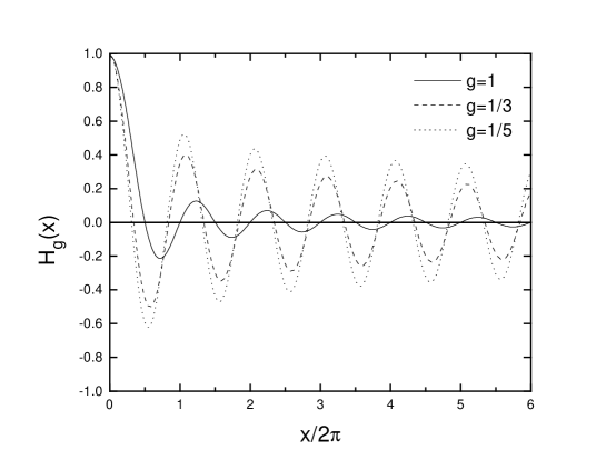
FIG. 2.: Modulation $H_{g}(x)$ for $g=1,1/3,1/5$. Notice that the decay rate of the modulation is $x^{-g}$. Also, the position of the zeros of $H_{g}(x)$ (those of $J_{g-1/2}(x)$) are approximately given by $x_{n}\approx\pi(n+\xi_{g})$, $n$ integer, where $\xi_{g}=\frac{1+g}{2}$ is a $g$ dependent shift

The zeros of $H_{g}(x)$ are those of the Bessel function $J_{g-1/2}(x)$, which are separated by a distance approximately equal to $\pi$. The zeros are approximately given by

$$x_{n}\approx\pi(n+\xi_{g})\ ,\ \ n=0,1,\dots\qquad{\rm with}\qquad\xi_{g}=\frac{1+g}{2}\ ,$$ (7)

which fits the graphs in Figure 2 very well. Notice that for $g=1$, the position of the zeros is exactly given by $x_{n}=\pi(n+1)$, $n=0,1,\dots$, and all zeros are equally spaced. The ratio $x_{1}/x_{0}$ between the first two zeros is 2. For $g\neq 1$, even though the zeros are approximately equally separated, they are shifted, and $x_{1}/x_{0}\approx\frac{g+3}{g+1}\neq 2$. This example illustrates how the position of the zeros can be used to probe Luttinger liquid behavior.

Experimentally, the position of these nodes can be observed precisely by measuring those source-drain voltages for which the Aharonov-Bohm oscillations simply disappear. We would like to stress that the experimental measurement of the position of the nodes of the interference patterns provides a clean (interferometric) way of probing Luttinger liquid behavior. Such an interferometric measurement focuses on the behavior between the two contacts, and may be free of parasitic effects elsewhere that can mask the anomalous scaling behavior of Luttinger liquids.

Finally, the location of the nodes could also provide another method of measuring fractional charge. The position of the nodes depends on $\omega_{J}a/v$, where the Josephson frequency $\omega_{J}=e^{*}V/\hbar$ depends on the fractional charge. If there were an independent measurement of the velocity the of edge modes $v$, then the location of the nodes would yield a value for $e^{*}$.

IV Free Fermions

To better understand the behavior of our perturbative solution for the current, we will look at the exact solution for the $g=1$ case with two constrictions. This case reduces to a simple problem that is essentially the same as wave transmission through a Fabry-Perot interferometer. We can solve for the transmission and reflection amplitudes at a single impurity, which, for $g=1$, are independent of the energy of the incident waves. Then, in addition to using these amplitudes to account for the scattering at each of the two impurities, we must also propagate the waves from one impurity to another, which is the part responsible for the interference effects. Each frequency $\omega$ will then be transmitted with a different coefficient $T(\omega)$. For an applied voltage $V$ between the edges, there will be a whole range of frequencies of width $\omega_{J}=eV/\hbar$ in the incident wave packet. We must then integrate the final transmission coefficients over the energies in this band that contribute to the total current.

Consider, to begin with, a single point-contact with tunneling amplitude $\Gamma$, which can either transmit or scatter a particle. For $g=1$, we can work in terms of free fermions given by $\psi_{R,L}={1\over\sqrt{2\pi}}e^{\pm i\phi_{R,L}(x,t)}$, with Hamiltonian

$$H=\int d x \bigg{\{}{\psi_{R}}^{\dagger}(x)\left[-i{\partial\over\partial x}-{\omega_{0}\over 2}\right]\psi_{R}(x)+{\psi_{L}}^{\dagger}(x)\left[i{\partial\over\partial x}+{\omega_{0}\over 2}\right]\psi_{L}(x)$$ (8)

$$+ 2\pi\delta(x)\left[\Gamma_{i}{\psi_{L}}^{\dagger}(x)\psi_{R}(x)+H.c.\right]\bigg{\}}.$$ (9)

Once again, we have set the velocity $v$ of the chiral fermions to 1. It is then a straightforward wave mechanics problem to solve for the scattering matrix, $S$, which gives the transformation from the incoming modes, $\tilde{\psi}_{R-}(\omega)$, $\tilde{\psi}_{L+}(\omega)$ to the outgoing modes, $\tilde{\psi}_{R+}(\omega)$, $\tilde{\psi}_{L-}(\omega)$. We find that $S=\pmatrix{t_{i}&r_{i}\cr-{r_{i}}^{*}&t_{i}\cr}$, where the transmission and reflection amplitudes are given by

$$t_{i}={1-\pi^{2}|\Gamma_{i}|^{2}\over 1+\pi^{2}|\Gamma_{i}|^{2}}\qquad{\rm and}\qquad r_{i}={-i2\pi{\Gamma_{i}}^{*}\over 1+\pi^{2}|\Gamma_{i}|^{2}}\ .$$ (10)

The transmission and reflection coefficients are $T=|t|^{2}$ and $R=|r|^{2}$, respectively. (We note here that $\Gamma_{i}$ in Equation 10 is renormalized so that the strong barrier limit or total reflection ($R=1$) occurs when $|\Gamma_{i}|=1/\pi$. This is in contrast with the case when $g=1/2$ or $1/3$, when total reflection occurs as $\Gamma\to\infty$. Technically, this difference arises because for $g<1$ the tunneling operator is infrared relevant whence short distance behavior does not matter, whereas for $g=1$ it is marginal.)

When there is more than one scatterer, it is convenient to use the transmission matrix approach to find the transmission through and reflection out of the two point-contacts separated by a distance $a$. Recall that the transmission matrix $M_{i}$ gives the transformation from the states on the left of the barrier, $\tilde{\psi}_{R-}(\omega)$, $\tilde{\psi}_{L-}(\omega)$, to the states on the right of the barrier, $\tilde{\psi}_{R+}(\omega)$, $\tilde{\psi}_{L+}(\omega)$, and can be obtained directly from $S$. After passing through the first constriction, the waves propagate to the right a distance $a$, which results in multiplying the modes $\pmatrix{\tilde{\psi}_{R}(\omega)\cr\tilde{\psi}_{L}(\omega)\cr}$ by $D=\pmatrix{e^{ia\omega}&0\cr 0&e^{-ia\omega}\cr}$. Finally, the waves are scattered again by the second point-contact, so the waves on the right-hand side depend on the waves to the left of the scatterers as follows:

$$\pmatrix{\tilde{\psi}_{R+}(\omega)\cr\tilde{\psi}_{L+}(\omega)\cr}=M_{2}DM_{1}\pmatrix{\tilde{\psi}_{R-}(\omega)\cr\tilde{\psi}_{L-}(\omega)\cr}.$$ (11)

Note that the matrix $D$ contains the phase $e^{\pm i\omega x}$, and it is this phase which is responsible for the voltage oscillations. In particular, the right-moving and left-moving modes that scatter between the two point-contacts have opposite phases which interfere with each other. Multiplying out the matrices in Eq. (11), we find that the transmission amplitude for the two point-contact geometry is

$$t(\omega)=\frac{t_{1}t_{2}}{1+r_{1}r^{*}_{2}e^{2i\omega a}}\ ,$$ (12)

where $t_{1,2}$ and $r_{1,2}$ are the transmission and reflection amplitudes for the two contacts, as given by Eq. (10). The transmission coefficient $T(\omega)$ through the whole droplet is then

$$T(\omega)=\frac{|t_{1}|^{2}|t_{2}|^{2}}{1+|r_{1}|^{2}|r_{2}|^{2}+(r_{1}r^{*}_{2}e^{2i\omega a}+r^{*}_{1}r_{2}e^{-2i\omega a})}\ .$$ (13)

With this frequency dependent transmission coefficient, we can calculate the current for an energy difference $\omega_{J}$ between the right and left moving edges. It is given by the total right-moving current minus the total left-moving current passing through a point $x$. If we choose the point to be to the right of the barrier, then the total right-moving current at energy $\omega$ is given by the transmitted right-moving current $e{\cal T}(\omega)n^{R}(\omega)$ plus the total left-moving current that was reflected into right movers $e[1-{\cal T}(\omega)]n^{L}(\omega)$. Similarly, the total left-moving current at energy $\omega$ is just the total incoming left-moving current $n^{L}(\omega)$, where $n^{R,L}(\omega)$ are the occupation numbers of right and left movers. In this simple model we can easily include the temperature dependence of the transmission because it can be completely accounted for by the Fermi-Dirac distribution of the left and right movers:

$$n^{R,L}(\omega)=\frac{1}{e^{\beta(\omega\mp\omega_{J}/2)}+1}\ .$$ (14)

The expression for the current through the droplet then reduces to

$$I=e\int_{-\infty}^{\infty}{d\omega\over 2\pi}T(\omega)\left[n^{R}(\omega)-n^{L}(\omega)\right]\ .$$ (15)

At zero temperature, the integral in Eq. (15) yields

$$I={e\over 2\pi a}{|t_{1}|^{2}|t_{2}|^{2}\over 1-|r_{1}|^{2}|r_{2}|^{2}}\tan^{-1}\left(\frac{{1-|r_{1}|^{2}|r_{2}|^{2}\over 1+|r_{1}|^{2}|r_{2}|^{2}}\sin(\omega_{J}a)}{\cos(\omega_{J}a)+{r_{1}r^{*}_{2}+r^{*}_{1}r_{2}\over 1+|r_{1}|^{2}|r_{2}|^{2}}}\right)\ .$$ (16)

Notice that if $t_{1}=t_{2}=1$ (total transmission), $I={e\over 2\pi}\omega_{J}={e^{2}\over h}V$. For small tunneling amplitutes $\Gamma_{1}$ and $\Gamma_{2}$ ($|r_{1}|^{2},|r_{2}|^{2}\ll 1$), we find that $I={e^{2}\over h}V-I_{t}$, where

$$I_{t}=e^{*}|\Gamma_{\rm eff}|^{2}\ 2\pi\omega_{J}\ ,$$ (17)

with

$$|\Gamma_{\rm eff}|^{2}=|\Gamma_{1}|^{2}+|\Gamma_{2}|^{2}+(\Gamma_{1}\Gamma^{*}_{2}+\Gamma^{*}_{1}\Gamma_{2})\ {\sin(\omega_{J}a)\over(\omega_{J}a)}\ .$$ (18)

This is the same as the result obtained perturbatively in section III if we set $g=1$ in Eq. (5).

If we expand the transmission coefficient $T(\omega)$ in Eq. (13) for small tunneling amplitudes, we can easily obtain the finite temperature tunneling current $I_{t}$. It is still given by Eq. (17), but the effective coupling is now

$$|\Gamma_{\rm eff}|^{2}=|\Gamma_{1}|^{2}+|\Gamma_{2}|^{2}+(\Gamma_{1}\Gamma^{*}_{2}+\Gamma^{*}_{1}\Gamma_{2})\ {2\pi Ta\over\sinh(2\pi Ta)}{\sin(\omega_{J}a)\over(\omega_{J}a)}\ .$$ (19)

Notice that the distance $a$ sets the temperature scale for which the interference term $\Gamma_{1}\Gamma^{*}_{2}+\Gamma^{*}_{1}\Gamma_{2}$ decays.

In the general case, such as for other filling fractions, the current should still be obtainable by an expression like Equation 15, where $T(\omega)$ is the transmission coefficient and $n^{R}(\omega)$ and $n^{L}(\omega)$ are the number densities of filled states at energy $\omega$. If the behavior of the system deviates from the result in Equation 16, this should indicate that the transmission and reflection amplitudes for a single point-contact depend on energy and that the density of states no longer has the simple Fermi-liquid form.

V Finite Temperature Effects

In section III we have found that, at zero temperature, the effect of the two point-contacts can be completely absorbed into an effective coupling $\Gamma_{\rm eff}$, which describes all the interference between the two contacts. In this section we will show that when $T\neq 0$, this is still the case, but now $\Gamma_{\rm eff}$ will depend on temperature also.

The finite temperature $T$ brings another energy scale to the problem. This energy scale should be compared to the one set by the separation between the contacts $a$, which is given by $\omega_{\rm osc}=2\pi v/a$. Thus, when $kT\gg\hbar\omega_{\rm osc}$, the interference effects should be washed out. One should also keep in mind the energy scale associated with the Josephson frequency $\omega_{J}=e^{*}V/\hbar$, so that the decay of the interference effects with temperature will depend on the ratios of the three energy scales $T$, $\omega_{J}$ and $\omega_{\rm osc}$. The interesting question to ask is how the different $g$ affect the way the interference is washed out, or, equivalently, how the filling factor $\nu$ of the underlying FQH state affects the decay of the oscillations with temperature.

To lowest order in the tunneling amplitude $\Gamma$, the tunneling current between edge states in the presence of a single point-contact at finite temperature is given by [17]:

$$I_{t}=e^{*}\ |\Gamma|^{2}4(\pi T)^{2g-1}\ B\left(g-i{\omega_{J}\over 2\pi T},g+i{\omega_{J}\over 2\pi T}\right)\sinh\left({\omega_{J}\over 2T}\right)\ ,$$ (20)

where $B$ is the beta function. In appendix A we show that the same expression gives the current for $N$ point-contacts with couplings $\Gamma_{i}$, $i=1,...,N$ if we use an effective coupling

$$|\Gamma_{\rm eff}|^{2}=\sum_{i,j=1}^{N}\Gamma_{i}\ \Gamma^{*}_{j}\ H_{g}(\omega_{J},|x_{i}-x_{j}|,T)\ ,$$ (21)

with

$$H_{g}(\omega_{J},x,T)=2\pi{\Gamma(2g)\over\Gamma(g)}{e^{-2g\pi T|x|}\over\sinh{\omega_{J}\over 2T}}\ \times\ {\rm Im}\bigg{\{}{e^{-i\omega_{J}|x|}\ F(g,g+i{\omega_{J}\over 2\pi T};1+i{\omega_{J}\over 2\pi T};e^{-4\pi T|x|})\over\Gamma(g-i{\omega_{J}\over 2\pi T})\ \Gamma(1+i{\omega_{J}\over 2\pi T})}\bigg{\}}\ .$$ (22)

In this expression, $F$ is a hypergeometric function. Notice that the function $H_{g}$ depends on $T$, $x$ and $\omega_{J}$ only through the combinations $\omega_{J}x$ and $\omega_{J}/(2\pi T)$. We can thus cast the modulation $H_{g}\left(\omega_{J}x,{\omega_{J}\over 2\pi T}\right)$ in terms of the following function of two variables:

$$H_{g}(y_{1},y_{2})=2\pi{\Gamma(2g)\over\Gamma(g)}{e^{-gy_{1}/y_{2}}\over\sinh(\pi y_{2})}\ \times\ {\rm Im}\bigg{\{}{e^{-iy_{1}}\ F(g,g+iy_{2};1+iy_{2};e^{-2y_{1}/y_{2}})\over\Gamma(g-iy_{2})\ \Gamma(1+iy_{2})}\bigg{\}}\ .$$ (23)

The effective coupling for a two point-contact geometry is then

$$|\Gamma_{\rm eff}|^{2}=|\Gamma_{1}|^{2}+|\Gamma_{2}|^{2}+(\Gamma_{1}\Gamma^{*}_{2}+\Gamma^{*}_{1}\Gamma_{2})\ H_{g}\left({2\pi\omega_{J}\over\omega_{\rm osc}},{\omega_{J}\over 2\pi T}\right)\ .$$ (24)

In this form, it is clear that the interference term depends on the ratios of the three energy scales in the problem.

We begin to explore how different values of $g$ change the behavior of the modulation $H_{g}$ by considering Fermi liquid ($g=1$) edge states associated with a QH filling factor $\nu=1$. In this case, Eq. (23) can be shown to simplify to

$$H_{1}(y_{1},y_{2})={y_{1}/y_{2}\over\sinh(y_{1}/y_{2})}{\sin y_{1}\over y_{1}}\ ,$$ (25)

so that

$$|\Gamma_{\rm eff}|^{2}=|\Gamma_{1}|^{2}+|\Gamma_{2}|^{2}+(\Gamma_{1}\Gamma^{*}_{2}+\Gamma^{*}_{1}\Gamma_{2})\ {4\pi^{2}T/\omega_{\rm osc}\over\sinh(4\pi^{2}T/\omega_{\rm osc})}\ {\sin(2\pi\omega_{J}/\omega_{\rm osc})\over(2\pi\omega_{J}/\omega_{\rm osc})}\ .$$ (26)

This is the same as the expression obtained in section IV directly from the free fermion transmission approach. Notice that for $g=1$ the finite temperature correction appears only as a multiplicative factor in front of the modulation for $T=0$. This is not necessarily the case for other $g$, as shown below in Fig. 4. This multiplicative factor decays exponentially ($1/\sinh(4\pi^{2}T/\omega_{\rm osc})$) with temperature, with the scale ($\omega_{\rm osc}$) set by the two point-contact separation $a$. In Fig. 3 we show the decay of $H_{g}$ with temperature for $\omega_{J}=0$ in a log-plot. From this plot we can extract how the modulation decays with temperature $T$ for different $g$. Using asymptotic expressions for the hypergeometric function, we find that for $T\gg\omega_{\rm osc}$, the function $H_{g}({2\pi\omega_{J}\over\omega_{\rm osc}},{\omega_{J}\over 2\pi T})$ decays as $e^{-4\pi^{2}gT/\omega_{\rm osc}}$, whereas for $T\ll\omega_{\rm osc}$, the fall off is much slower.

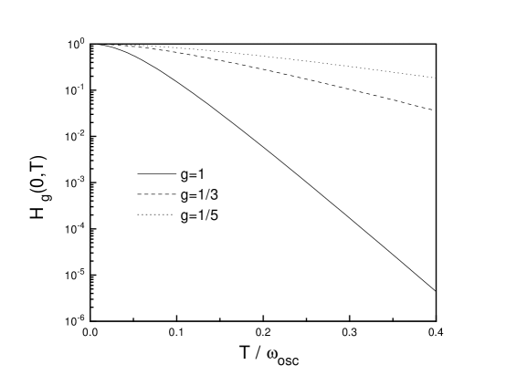
FIG. 3.: Temperature decay of the modulation $H_{g}$ for $g=1,1/3,1/5$. The quantity plotted is $H_{g}(\omega_{J}=0,a,T)$ vs. $T$, with $T$ measured in units of $\omega_{\rm osc}=2\pi\frac{v}{a}$ (the energy scale associated with the point-contact separation $a$). Notice that the modulation decays exponentially with $T$ for large temperatures, and that the decay rate is faster for larger $g$.

Another interesting quantity is presented in Fig. 4, where we display the ratio $H_{g}(\omega_{J},a,T)/H_{g}(0,a,T)$ between the modulation at $\omega_{J}$ and at $\omega_{J}=0$, for different temperatures. The natural variables for displaying this dependence are the ratios $T/\omega_{\rm osc}$ and $\omega_{J}/\omega_{\rm osc}$ (put differently, we measure energies as compared to the scale $\omega_{\rm osc}$ set by the separation $a$ between the contacts). Notice that, for general $g$, the curves move around as a function of $T$. The curves collapse into one only for $g=1$. Also notice that as the temperature increases, the position of the zeros for $g=1/3$ and $g=1/5$ approaches those for $g=1$, so that increasing temperature masks the Luttinger liquid behavior, with a crossover temperature roughly equal to $\omega_{\rm osc}$.

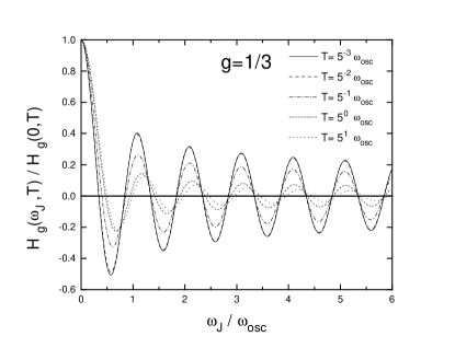
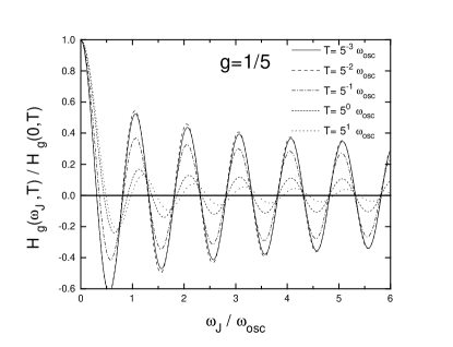
FIG. 4.: Dependence of the modulation $H_{g}(\omega_{J},a,T)$ on $\omega_{J}$ for different $T$. The quantity plotted is the rescaled $H_{g}$ ($H_{g}(\omega_{J},a,T)/H_{g}(0,a,T)$) so as to show how the shape of the modulation curve changes with $T$ for different $g$. Notice that all curves collapse for $g=1$, i.e., all frequencies get suppressed uniformly as temperature is increased. For $g=1/3$ and $g=1/5$, however, notice that the curves do not collapse together anymore, and that higher $\omega_{J}$ are supressed more strongly than lower $\omega_{J}$ as $T$ is increased.

VI Numerical Estimates

In this section, we will give estimates of the sizes of parameters at which the interference effects could be observed. First, we will consider the change in magnetic field, $\Delta B$, required for one Aharonov-Bohm period, which is given by

$$\Delta B={\ e\ \over\ e^{*}}{\Phi_{0}\over A}={\ e\ \over\ e^{*}}{41\mu{\rm m}^{2}\ {\rm gauss}\over A}.$$ (27)

If the number of electrons is held constant, then in this equation $\Phi_{0}$ is equal to one flux quantum and $e^{*}$ is the charge of an electron, $e$. If, instead, the filling fraction is held fixed, then $\Phi_{0}$ is $e/e^{*}$ times one flux quantum, where $e^{*}$ is the charge of the quasiparticle. In this equation, $A$ is the area of the FQH liquid between the two contacts, and is roughly given by $A=ad$, where $d$ is the width of the sample and $a$ is the distance between the two contacts. If we assume the width is $d=1\mu{\rm m}$, then the period is related to the distance between the contacts by

$$\Delta B=\cases{41\mu{\rm m-gauss}/a&for fixed number of electrons $n$\cr 120\mu{\rm m-gauss}/a&for fixed filling fraction $\nu=1/3$.}$$ (28)

For $a=1\mu{\rm m}$ or $10\mu{\rm m}$, the “electron” Aharonov-Bohm period is $\Delta B=41$ gauss and $4.1$ gauss, respectively, and the “quasiparticle” Aharonov-Bohm period is $\Delta B=120$ gauss and $12$ gauss, respectively.

Next, we consider the voltage fluctuations. The separation between the zeros of the Bessel function $J_{g-1/2}(x)$ is approximately equal to $\pi$ and the location of the nodes in the voltage fluctuations roughly occur when

$${\omega_{J}a\over v}\approx\pi(n+\xi_{g})\ ,\ \ n=0,1,\dots\qquad{\rm with}\qquad\xi_{g}=\frac{1+g}{2}\ ,$$ (29)

As noted earlier, depending on the value of $g$, the precise location of these nodes will be shifted a little, which may provide a way of distinguishing between Luttinger liquid behavior and other types of behavior. In this equation, we have restored the velocity of the edge modes $v$, which earlier was set to 1. For $g=1/3$, an estimate for $v$ [32] is $v\approx 10^{5}{\rm m}/{\rm s}$. Using $\omega_{J}=e^{*}V/\hbar$, we find that the voltage at the nodes and the distance between the point-contacts must satisfy

$$Va=(n+\xi_{g}){e\over e^{*}}\times 200\mu{\rm V}-\mu{\rm m},$$ (30)

where $V$ has units of microvolts and $a$ has units of microns. For $\nu=1/3$, we take $e^{*}/e=1/3$. Thus, for $a=1\mu{\rm m}$ or $10\mu{\rm m}$ the voltage at the first node is roughly $400\mu{\rm V}$ and $40\mu{\rm V}$, respectively. Lastly, we will estimate the coherence length, or the amount by which the temperature reduces the signal. However, we note that phonons can also lead to dephasing, althought we do not consider them here. For temperatures greater than $kT>\hbar\omega_{\rm osc}/(4\pi^{2})$, the interference effects fall off as $Te^{-4\pi^{2}gkT/(\hbar\omega_{\rm osc})}$, where $\omega_{\rm osc}=2\pi v/a$. Thus, for

$$kT<{\hbar v\over 2\pi ga}$$ (31)

the signal is not affected much by temperature. We can define the coherence length, $a_{c}$ by the spacing for which the signal has decreased roughly by a factor of $1/e$, so that $a_{c}=v\hbar/(g2\pi kT)$. Then, for $v\approx 10^{5}{\rm m}/{\rm s}$ and $g=1/3$, at $T=100{\rm mK}$ the coherence length is $a_{c}=4\mu{\rm m}$, and for $T=30{\rm mK}$, the coherence length is $a_{c}=12\mu{\rm m}$. Thus, the signal for a separation of $1\mu{\rm m}$ should not be noticeably affected at either temperature, and even for a separation of $10\mu{\rm m}$ the signal will be attenuated by a factor of 2 at $30{\rm mK}$ and by a factor of 15 at $100{\rm mK}$.

It follows then that a separation of a few microns should be sufficient to allow observation of the inteference effects at temperatures around and below $100{\rm mK}$. The requirement on the gates is that they be close enough that their electrostatic “shadows” do not overlap in the plane of the electron gas. For gate diameters of about $1000\AA$, this condition could be met by placing them about $1000\AA$ from the electron gas.

VII Conclusions

In this paper we have proposed a device, the two point-contact interferometer, consisting of a Hall bar with two weak barriers, that can be used to study quantum interference effects in a strongly correlated system. The device allows for the study of three types of interference effects: Aharanov-Bohm oscillations with magnetic field, statistical oscillations with quasiparticle number and Fabry-Perot oscillations with source-drain voltage. These interference effects can be used to measure the fractional charge and statistics of quasiparticles in the quantum Hall effect. They also provide a new way of searching for non-Fermi liquid behavior in the dynamics of the edges. We would like to emphasize that much of our account of the physics of the device is quite robust, in that it depends upon quite general “topological” properties of QH quasiparticles; our proposals for measuring charge and statistics fall in this category. Other features, such as the details of the Fabry-Perot nodes are more specific to the simplest version of edge state dynamics used in the calculations and as such are subject to the caveat that they represent the behavior of the system only at the lowest energies.

ACKNOWLEDGEMENTS

We would like to thank several colleages who gave us important suggestions and constructive criticism on the experimental implications of this work: David Abusch-Magder, Ray Ashoori, Marc Kastner, Beth Parks and Nikolai Zhitenev at MIT; Hari Manoharan, Kathryn Moler, Dan Shahar, Mansour Shayegan and Lydia Sohn at Princeton; Hong-Wen Jiang at UCLA. SLS would like to thank Phillip Phillips for introducing him to resonances in interacting systems and for suggesting that the two barrier problem might be a good thing to look at. This work is supported by NSF grants DMR-94-00334 (CCC), DMR-93-12606 (SAK) and DMR-94-11574 (XGW). XGW and SLS acknowledge support from the A. P. Sloan Foundation. D. F. is currently a Bunting Fellow sponsored by the Office of Naval Research.

A perturbative calculation

We derive here the correction to the Hall current due to tunneling at the point-contacts. We will assume the general case of $N$ contacts at locations $x_{i}$ and coupling $\Gamma_{i}$, $i=1,...,N$.

The first step in the calculation is to obtain the tunneling current operator $j(t)$. This operator includes the tunneling currents flowing from one edge to the other through all $N$ point-contacts in the problem. The tunneling operator can be obtained from the time evolution of the total charge operators $Q_{R,L}$ on the $R,L$ edges:

$$j(t)=-\frac{1}{i\hbar}[Q_{L},H]=\frac{1}{i\hbar}[Q_{R},H]\ .$$ (A1)

The charge operator commutes with the free part of the Hamiltonian, so that the only contribution comes from the tunneling term

$$H_{\rm tun}=\sum_{i=1}^{N}\Gamma_{i}e^{-i\omega_{J}t}e^{i\sqrt{g}\phi(t,x_{i})}+H.c.\ .$$ (A2)

Using the commutation relations for the bosonic fields $\phi_{R,L}$, we obtain

$$j(t)=ie^{*}\sum_{i=1}^{N}\Gamma_{i}e^{i\sqrt{g}\phi(t,x_{i})}+H.c.\ .$$ (A3)

The expectation value for the current at time $t$ is given by

$$\langle j(t)\rangle=\langle 0|S^{\dagger}(t,-\infty)\ j(t)\ S(t,-\infty)|0\rangle\ ,$$ (A4)

where $S(t,-\infty)$ is the time evolution operator. The next step is to calculate $\langle j\rangle$ perturbatively in the tunneling amplitudes $\Gamma_{i}$. Because there is a voltage difference between the $R$ and $L$ terminals, the system is out of thermodynamical equilibrium, and we must to use field theoretical tools appropriate for such non-equilibrium problems [18]. However, non-equilibrium effects appear only to second and higher orders in perturbation theory. Because we will calculate the tunneling current only to first order in perturbation theory, we will not have to use non-equilibrium field theory in this particular calculation.

To lowest order in the tunneling perturbation we have

$$\langle j(t)\rangle=-i\int_{-\infty}^{t}\ dt^{\prime}\ \langle 0|[j(t),H_{\rm tun}(t^{\prime})]|0\rangle\ .$$ (A5)

In the calculation of

$$\langle 0|j(t)\ H_{\rm tun}(t^{\prime})|0\rangle = e^{*}\sum_{i=1}^{N}\sum_{j=1}^{N}\ \langle 0|(i\Gamma_{i}e^{-i\omega_{J}t}e^{i\sqrt{g}\phi(t,x_{i})}-i\Gamma_{i}^{*}e^{i\omega_{J}t}e^{-i\sqrt{g}\phi(t,x_{i})})$$ (A6)

$$\ \ \ \ \ \ \ \ \ \ \times\ (\Gamma_{j}e^{-i\omega_{J}t^{\prime}}e^{i\sqrt{g}\phi(t^{\prime},x_{j})}+\Gamma_{j}^{*}e^{i\omega_{J}t^{\prime}}e^{-i\sqrt{g}\phi(t^{\prime},x_{j})})|0\rangle$$ (A7)

the non-vanishing terms are those that transfer zero total charge when applied to $|0\rangle$. We then have

$$\langle 0|j(t)\ H_{\rm tun}(t^{\prime})|0\rangle=$$ (A8)

$$=ie^{*}\sum_{i,j=1}^{N}\Big{(}\Gamma_{i}\Gamma_{j}^{*}\ e^{-i\omega_{J}(t-t^{\prime})}\langle 0|e^{i\sqrt{g}\phi(t,x_{i})}e^{-i\sqrt{g}\phi(t^{\prime},x_{j})}|0\rangle-\Gamma_{i}^{*}\Gamma_{j}\ e^{i\omega_{J}(t-t^{\prime})}\langle 0|e^{-i\sqrt{g}\phi(t,x_{i})}e^{i\sqrt{g}\phi(t^{\prime},x_{j})}|0\rangle\Big{)}$$ (A9)

$$=ie^{*}\sum_{i,j=1}^{N}\ (\Gamma_{i}\Gamma_{j}^{*}\ e^{-i\omega_{J}(t-t^{\prime})}-\Gamma_{i}^{*}\Gamma_{j}\ e^{i\omega_{J}(t-t^{\prime})})\ e^{g\langle 0|\phi(t,x_{i})\phi(t^{\prime},x_{j})|0\rangle}\ .$$ (A10)

The $\phi$ field correlation is

$$\langle 0|\phi(t,x)\phi(0,0)|0\rangle = \langle 0|\phi_{R}(t,x)\phi_{R}(0,0)|0\rangle+\langle 0|\phi_{L}(t,x)\phi_{L}(0,0)|0\rangle$$ (A11)

$$= -\ln[\delta+i(t-x)]-\ln[\delta+i(t+x)]\ ,$$ (A12)

where $\delta$ is an ultraviolet cut-off scale. Let us define

$$P_{g}(t,x)=e^{g\langle 0|\phi(t,x)\phi(0,0)|0\rangle}=\big{[}\delta+i(t+x)\big{]}^{-g}\times\big{[}\delta+i(t-x)\big{]}^{-g}\ .$$ (A13)

Notice that $P_{g}(t,x)=P_{g}(t,-x)$. Using the expression above, we can write

$$-i\langle[j(t),H_{\rm tun}(t^{\prime})]\rangle = e^{*}\sum_{i,j=1}^{N}\ \left(\Gamma_{i}\Gamma_{j}^{*}\ e^{-i\omega_{J}(t-t^{\prime})}-\Gamma_{i}^{*}\Gamma_{j}\ e^{i\omega_{J}(t-t^{\prime})}\right)$$ (A14)

$$\ \ \times\ \Big{(}P_{g}(t-t^{\prime},x_{i}-x_{j})-P_{g}(-t+t^{\prime},x_{i}-x_{j})\Big{)}\ .$$ (A15)

Inserting the above expression into Eq.(A5) and performing the $t^{\prime}$ integration, we obtain the current expectation value:

$$\langle j(t)\rangle = e^{*}\sum_{i,j=1}^{N}\ {\Gamma_{i}\Gamma_{j}^{*}+\Gamma_{i}^{*}\Gamma_{j}\over 2}\ [{\tilde{P}_{g}}(\omega_{J},x_{i}-x_{j})-{\tilde{P}_{g}}(-\omega_{J},x_{i}-x_{j})]\ ,$$ (A16)

where ${\tilde{P}}_{g}(\omega_{J},x)$ is the Fourier transform of the $P_{g}(t,x)$ with respect to time. The problem is then reduced to the calculation of the ${\tilde{P}}_{g}$’s. It is easy to calculate

$${\tilde{P}_{g}(\omega,0)}=\int_{-\infty}^{\infty}dp\frac{e^{i\omega p}}{(\delta+ip)^{2g}}=\frac{2\pi}{\Gamma(2g)}|\omega|^{2g-1}e^{-|\omega|\delta}\ \theta(\omega)\ ,$$ (A17)

and we can express the case $x\neq 0$ in terms of the ${\tilde{P}_{g}(\omega,0)}$:

$${\tilde{P}_{g}(\omega,x)} = \int_{-\infty}^{\infty}{d\omega^{\prime}\over 2\pi}\ P_{g/2}(\omega^{\prime},0)\ P_{g/2}(\omega-\omega^{\prime},0)\ e^{-i(2\omega^{\prime}-\omega)x}$$ (A18)

$$= \theta(\omega)\ \int_{0}^{|\omega|}{d\omega^{\prime}\over 2\pi}\ \omega^{\prime g-1}\ (\omega-\omega^{\prime})^{g-1}\ e^{-i(2\omega^{\prime}-\omega)x}$$ (A19)

$$= {\tilde{P}}_{g}(\omega,0)\ H_{g}(\omega x)\ ,$$ (A20)

where

$$H_{g}(y)=\sqrt{\pi}\ {\Gamma(2g)\over\Gamma(g)}\ {J_{g-1/2}(y)\over(2y)^{g-1/2}}\ .$$ (A21)

The tunneling current between the edge states $I_{t}=\langle j(t)\rangle$ is then simply

$$I_{t}=e^{*}{2\pi\over\Gamma(2g)}|\omega_{J}|^{2g-1}\ {\rm sign}(\omega_{J})\ \sum_{i,j=1}^{N}\Gamma_{i}\Gamma_{j}^{*}\ H_{g}(\omega|x_{i}-x_{j}|)\ .$$ (A22)

The expression for the tunneling current can be cast exactly in the same form as that for a single contact,

$$I_{t}=e^{*}|\Gamma_{\rm eff}|^{2}\ {2\pi\over\Gamma(2g)}|\omega_{J}|^{2g-1}\ {\rm sign}(\omega_{J})\ ,$$ (A23)

but with an effective coupling $\Gamma_{\rm eff}$ due to the interference between $\Gamma_{i}$, $i=1,..,N$ of the $N$ contacts:

$$|\Gamma_{\rm eff}|^{2}=\sum_{i,j=1}^{N}\Gamma_{i}\ \Gamma^{*}_{j}\ H_{g}(\omega_{J}|x_{i}-x_{j}|)\ .$$ (A24)

The calculations for $T=0$ can be extended for finite temperature. Basically, the algebraic correlations at $T=0$ are mapped to the correlations at $T\neq 0$ by a conformal transformation [31]:

$$\frac{1}{[\delta+i(t\pm x)]^{g}}\rightarrow\left[\frac{\pi T}{\sin\left(\pi T[\delta+i(t\pm x)]\right)}\right]^{g}\ .$$ (A25)

Using this transformation, we can recalculate the ${\tilde{P}_{g}}$’s and obtain their finite $T$ version:

$${\tilde{P}_{g}(\omega,x,T)} = \int_{-\infty}^{\infty}dt\ e^{i\omega t}\left[\frac{\sin\left(\pi T[\delta+i(t+x)]\right)}{\pi T}\right]^{-g}\left[\frac{\sin\left(\pi T[\delta+i(t-x)]\right)}{\pi T}\right]^{-g}$$ (A26)

$$= (\pi T)^{2g}\int_{-\infty}^{\infty}dt\ e^{i\omega t}\ e^{-i\frac{\pi}{2}g[{\rm sign}(t-x)+{\rm sign}(t+x)]}\bigg{[}\sinh(\pi T|t-x|)\sinh(\pi T|t+x|)\bigg{]}^{-g}\ .$$ (A27)

What we need for the calculation of the currents is the difference ${\tilde{P}_{g}(\omega,x,T)}-{\tilde{P}_{g}(-\omega,x,T)}$, which simplifies to

$${\tilde{P}_{g}(\omega,x,T)}-{\tilde{P}_{g}(-\omega,x,T)}=4(\pi T)^{2g}\ \sin(\pi g)\ {\rm Im}\bigg{\{}\int_{|x|}^{\infty}dt\ e^{-i\omega t}\bigg{[}\sinh(\pi T|t-x|)\sinh(\pi T|t+x|)\bigg{]}^{-g}\bigg{\}}\ .$$ (A28)

After calculating the integral above, we find that it can be written as

$${\tilde{P}_{g}(\omega,x,T)}-{\tilde{P}_{g}(-\omega,x,T)}=\left[{\tilde{P}_{g}(\omega,x=0,T)}-{\tilde{P}_{g}(-\omega,x=0,T)}\right]\ \times\ H_{g}(\omega,x,T)\ ,$$ (A29)

where the $x=0$ difference is

$${\tilde{P}_{g}(\omega,x=0,T)}-{\tilde{P}_{g}(\omega,x=0,T)}=4(\pi T)^{2g-1}\ B\left(g-i{\omega\over 2\pi T},g+i{\omega\over 2\pi T}\right)\cosh\left({\omega\over 2T}\right)\ ,$$ (A30)

and the scaling factor $H_{g}(\omega,x,T)$ for $x\neq 0$ is

$$H_{g}(\omega,x,T)=2\pi{\Gamma(2g)\over\Gamma(g)}{e^{-2g\pi T|x|}\over\sinh{\omega\over 2T}}\ \times\ {\rm Im}\bigg{\{}{e^{i\omega|x|}\ F(g,g-i{\omega\over 2\pi T};1-i{\omega\over 2\pi T};e^{-4\pi T|x|})\over\Gamma(g+i{\omega\over 2\pi T})\ \Gamma(1-i{\omega\over 2\pi T})}\bigg{\}}\ ,$$ (A31)

where $F$ is the hypergeometric function.

Again, the tunneling current can be written as the tunneling through a single contact:

$$I_{t}=e^{*}|\Gamma_{\rm eff}|^{2}\ 4(\pi T)^{2g-1}\ B\left(g-i{\omega\over 2\pi T},g+i{\omega\over 2\pi T}\right)\sinh\left({\omega\over 2T}\right)\ ,$$ (A32)

but with an effective coupling

$$|\Gamma_{\rm eff}|^{2}=\sum_{i,j=1}^{N}\Gamma_{i}\ \Gamma^{*}_{j}\ H_{g}(\omega_{J},|x_{i}-x_{j}|,T)\ ,$$ (A33)

much in the same way as in the $T=0$ case.

REFERENCES

- [1] For a review, see Mesoscopic Phenomena in Solids, edited by B. L. Altshuler, P. A. Lee, and R. A. Webb (Elsevier, Amsterdam, 1990).
- [2] R. B. Laughlin, Phys. Rev. Lett. 50, 1395 (1983).
- [3] B. I. Halperin, Phys. Rev. Lett. 52, 1583 (1984).
- [4] D. Arovas, J. R. Schrieffer, and F. Wilczek, Phys. Rev. Lett. 53, 722 (1984).
- [5] T. Einarsson, S. L. Sondhi, S. M. Girvin, and D. P. Arovas, Nucl. Phys. B, 441, 515 (1995).
- [6] X. G. Wen and A. Zee, Phys. Rev. Lett. 69, 953 (1992)(E); Phys. Rev. Lett. 69, 3000 (1992).
- [7] D. H. Lee and X. G. Wen, Phys. Rev. B 49, 11066 (1994).
- [8] X. G. Wen, Phys. Rev. B 41, 12838 (1990).
- [9] S. A. Kivelson and V. L. Pokrovsky, Phys. Rev. B 40, 1373 (1989).
- [10] Steven Kivelson, Phys. Rev. Lett. 65, 3369 (1990).
- [11] V. L. Pokrovsky and L. P. Pryadko, Phys. Rev. Lett. 72 124 (1994).
- [12] J. A. Simmons, H. P. Wei, L. W. Engel, D. C. Tsui, and M. Shayegan, Phys. Rev. Lett. 63 1731 (1989).
- [13] V. J. Goldman and B. Su, Science, 267 1010 (1995).
- [14] D. R. Mace, C. H. W. Barnes, C. J. B. Ford, P. J. Simpson, M. Pepper, M. Y. Simmons, G. Faini, and D. Mailly, Proceedings of the 22nd International Conference on the Physics of Semiconductors, vol. 3, p. 1991 (1995).
- [15] A. S. Goldhaber and S. A. Kivelson, Phys. Lett. B 255, 445 (1991).
- [16] C. L. Kane and Matthew P. A. Fisher, Phys. Rev. Lett. 72, 724 (1994).
- [17] X. G. Wen, Phys. Rev. B 44, 5708 (1991).
- [18] C. de C. Chamon, D. E. Freed, and X. G. Wen, Phys. Rev. B 51, 2363 (1995).
- [19] C. de C. Chamon, D. E . Freed, and X.G. Wen, Phys. Rev. B 53, 4033 (1996).
- [20] P. Fendley, A. W. W. Ludwig, and H. Saleur, Phys. Rev. Lett. 75, 2196 (1995).
- [21] J. K. Jain, S. A. Kivelson, and D. J. Thouless, Phys. Rev. Lett., 71, 3003 (1993).
- [22] Xiao-Gang Wen, Intl. J. of Mod. Phys. B 6, 1711 (1992).
- [23] C. L. Kane and Matthew P. A. Fisher, Phys. Rev. Lett. 68, 1220 (1992); Phys. Rev. B 46, 15233 (1992); Phys. Rev. Lett. 72, 724 (1994).
- [24] Michael R. Geller, Daniel Loss, and George Kirczenow, cond-mat/9606070.
- [25] Xiao-Gang Wen, Phys. Rev. lett. 64, 2206 (1990).
- [26] A. Yariv Optical Electronics, Holt, Rinehart and Winston, New York , 1985.
- [27] F. P. Milliken, C. P. Umbach and R. A. Webb, Solid State Comm. 97, 309 (1995).
- [28] Here we are clearly assuming that the edge modes have a linear dispersion on an energy scale on which there is significant variation in the transmission; otherwise the lineshape with will be distorted.
- [29] Alternatively, one can account for Aharonov-Bohm and fractional statistics oscillations within the scope of edge state theory [8]; they can be absorbed into the relative phase between the two tunneling amplitudes and across the contacts of the interferometer. It is thus sheer question of taste as to which framework one chooses to use: that which focuses on the bulk, or that which looks at the boundary.
- [30] In writing this form, we have assumed that there is no significant energy dependence of the quasiparticle tunneling at the (low) energies of interest. This is problematic only in our analysis of the Fabry-Perot oscillations where a range of energies enter and the absolute location of the (AB) nodes is sensitive to this assumption. While this will require a quantitative assesment for realistic devices, we should note that regardless, a comparision between integer and fractional states could well serve as a diagnostic of Luttinger liquid behavior in the latter.
- [31] R. Shankar, J. Mod. Phys. B 4, 2371 (1990).
- [32] K. Moon and S. M. Girvin, cond-mat/9511013.