Towards Granular Hydrodynamics in Two-Dimensions

Abstract

We study steady-state properties of inelastic gases in two-dimensions in the presence of an energy source. We generalize previous hydrodynamic treatments to situations where high and low density regions coexist. The theoretical predictions compare well with numerical simulations in the nearly elastic limit. It is also seen that the system can achieve a nonequilibrium steady-state with asymmetric velocity distributions, and we discuss the conditions under which such situations occur.

PACS numbers: 05.20.Dd, 47.50.+d, 81.35.+k

I Introduction

Granular materials such as sand and powders have generated much interest of late. Such an ensemble of particles with macroscopic size is challenging since it may behave as a solid, a liquid or a gas. Size separation, pattern formation, avalanches, compaction and convection are just a few examples of the wide array of observed phenomena[1].

Flow underlies most of these phenomena and therefore, theoretical studies so far focus on formulating a hydrodynamical description appropriate to sand[2, 3]. These theories, stemming from the Boltzmann Equation, depend on the assumption of “molecular chaos”, i.e., the assumption that no interparticle correlations exist. This assumption is far from obvious. As a dissipative dynamical system, a granular system has attractors in its phase space, which may cause correlations between particles. Under certain conditions, these attractors lead to a singularity, inelastic collapse, which can not be explained by hydrodynamics. In one dimension, these attractors are so strong that hydrodynamics breaks down for the entire parameter space[4, 5]—in a confined geometry, all particles, save one, form a practically stationary clump against the elastic wall, while the remaining particle moves rapidly back and forth between the clump and the heated wall. Such a state clearly violates partition of energy.

In this study, we investigate the corresponding situation in two-dimensions[6, 7]. We consider inelastic hard spheres in a box where one wall is kept at a fixed temperature and the other three are reflecting (see Fig. 1). Energy input at the heated wall balances the dissipation due to inter-particle collisions and the system can achieve a steady state. Unlike the one-dimensional situation, the density and the temperature profiles are smooth functions of the distance from the heated wall. In the steady-state, the momentum balance equations imply that the pressure is constant throughout the system. Particles move faster close to the energy source and more slowly deeper inside the system due to energy loss. Thus the density is greater farther away from the wall to maintain a constant pressure.

Density variations may be a consequence of the above mechanism or an effect of the intrinsic attractors in the system which build up correlations among particles. Assuming that the particles are not coherent in the quasi-elastic limit, we derive a differential equation that describes the density variation throughout the system. Heuristic expressions for the mean-free path, the equation of state, and the thermal conductivity are incorporated into the energy flux balance equation to obtain a closed equation describing the steady-state density profiles. The theory compares well with simulational results over a wide range of densities in the quasi-elastic limit.

FIG. 1.: The system of interest. The length of the system is $L$, the width is $W$. The heated wall is at $x=0$; the elastic walls are at $x=L$, $y=0$, and $y=W$.

Our theory is appropriate for a steady-state which is very close to an equilibrium state. We expect this to be applicable only in the nearly elastic limit. We argue that in the complementary situation of stronger inelasticity, hydrodynamics may still be relevant. To analyze the nature of the steady-state, we study velocity distributions throughout the system. We observe that the velocity distributions exhibit scaling. This observation is then used to obtain a qualitative description of the behavior of the system.

II The quasi-elastic limit

Granular materials are different from ordinary fluids or gases in that the diameter of a particle may be comparable to the collisional mean free path. To formulate a hydrodynamic theory, it is necessary to describe how the mean free path, the pressure, and the thermal diffusivity depend on the grain diameter, the number density, and the temperature. In this section, we obtain heuristic expressions for these quantities.

Let us denote the number density of grains by $\rho$, the mean free path by $l$, and the grain diameter by $d$. Without loss of generality, we set the particle mass and the Boltzmann constant to unity: $m=k_{B}=1$. The granular temperature can be defined as the average kinetic energy per particle: $T\equiv\frac{1}{2}\langle v^{2}\rangle$. This quantity is well defined for an equilibrium state in which the particles have a symmetric velocity distribution. In such a case, $\bar{v}=\sqrt{2T}$, can be used as an approximate value for the average grain speed. In our system, quantities such as temperature, density, etc., are position dependent, and there is not a global equilibrium. However, in the quasi-elastic limit, we expect the system to be very close to local thermal equilibrium.

Let $x$ be the distance from the heated wall. In the steady state, all quantities vary only in this transverse direction. The energy balance equation can therefore be written

$$\frac{dq}{dx}+I=0,$$ (1)

where $q$ is the energy flux in the $x$ direction. The sink term $I$ accounts for the energy lost per unit area per unit time due to inelastic collisions. The energy flux is induced by a temperature gradient, $q=-\kappa dT/dx$, where the coefficient of thermal diffusivity, $\kappa$, is positive. Consequently, we find

$$\frac{d}{dx}\left(\kappa\frac{dT}{dx}\right)=I.$$ (2)

A The Energy Sink

Since collisions between grains are inelastic, kinetic energy is continually transferred into heat. For simplicity we neglect rotation and thus, the degree of inelasticity can be parameterized by $0\leq r\leq 1$. When two particles collide, their tangential velocities are unchanged, while the relative normal velocity is decreased by a factor of $-r$, where the negative sign merely indicates that they move apart after a collision. Using momentum conservation one can write the final velocities (indicated by primes) in terms of the initial velocities

$$\left(\begin{array}[]{c}v_{1n}^{\prime}\\ v_{2n}^{\prime}\end{array}\right)=\frac{1}{2}\left(\begin{array}[]{cc}1-r&1+r\\ 1+r&1-r\end{array}\right)\left(\begin{array}[]{c}v_{1n}\\ v_{2n}\end{array}\right).$$ (3)

In the above equation, the subscript $n$ denotes the velocity component along the line connecting the centers of particles 1 and 2. The energy lost in each collision is therefore

$$\Delta E=-\frac{1}{4}(1-r^{2})(v_{1n}-v_{2n})^{2}.$$

In this study, we focus on the quasi-elastic limit, i.e. $1-r\ll 1$. Physically, this limit is relevant to hard particles such as glass or steel beads.

Using the above expression for the energy dissipated in each collision, one can estimate the sink term, $I$, the mean energy lost per unit area per unit time. Consider a particle moving with speed $\bar{v}$. During each collision, it loses, on average, energy proportional to $(1-r^{2})\bar{v}^{2}$. In unit time, it collides roughly $\bar{v}/l$ times. In unit area, there are $\rho$ particles, and consequently

$$I\propto(1-r^{2})\bar{v}^{2}\frac{\bar{v}}{l}\rho\propto(1-r^{2})\rho T^{3/2}/l.$$

B The Coefficient of Thermal Diffusivity

Suppose there is a temperature gradient in the $x$-direction. As a result, there will be an energy flux along this axis. To calculate this flux, let us consider the number of particles crossing a line perpendicular to this direction in a time interval $\Delta t$. We define “crossing the line” as having any part of the particle over the line during this time interval. To cross the line within $\Delta t$, a particle with speed $\bar{v}$ must have its rightmost point $\bar{v}\Delta t$ or closer to the line. Thus, only grains in an area ($d+\bar{v}\Delta t$) to the left of the line can pass the line from the left in $\Delta t$. In fact, only one half of these particles are moving to the right, so the number of particles crossing the line per unit cross-sectional length in $\Delta t$ is $\frac{1}{2}\rho(d+\bar{v}\Delta t)$. In a steady state, the number of crossing events from each side must balance. Any energy flux is due to the fact that particles coming from the right are at a different temperature ($T_{R}$) than those from the left ($T_{L}$) and thus, $q\Delta t=\frac{1}{2}\rho(d+\bar{v}\Delta t)(T_{L}-T_{R})$. Consider two grains on opposite sides of the line. Their centers are approximately a distance $(l+d)$ apart, so the temperature difference is roughly $(l+d)dT/dx$. The coefficient of thermal conductivity is therefore $\kappa=-q/(dT/dx)=\frac{1}{2}\rho(l+d)(d+\bar{v}\Delta t)/\Delta t$. A natural choice for $\Delta t$ is the typical collision time $l/\bar{v}$. This choice is small enough to avoid multicounting and is sufficiently large to ensure that heat transfer does occur. Our heuristic picture therefore estimates the thermal diffusivity by

$$\kappa\propto\frac{\rho(l+d)^{2}\sqrt{T}}{l}.$$

This is a rough approximation; the actual prefactors depend on the velocity distribution of the grains. Therefore, we generally assume

$$\kappa\propto\frac{\rho(\alpha l+d)^{2}\sqrt{T}}{l}.$$

The energy balance equation (2) takes the form

$$\frac{d}{dx}\left[\frac{(\alpha l+d)^{2}}{l}\rho\sqrt{T}\frac{dT}{dx}\right]=(1-r^{2})\frac{\rho T^{\frac{3}{2}}}{\gamma l}$$ (4)

where $\gamma$ is the ratio of prefactors in the expressions for $I$ and $\kappa$. In the following subsections, we discuss how to obtain the dimensionless coefficients $\alpha$ and $\gamma$ self-consistently. To proceed, it is necessary to relate $\rho$ and $T$ through the equation of state. Additionally, the mean free path $l$ must be expressed in terms of $\rho$.

C The Equation of State

For the system to be in a steady state, the pressure must be constant throughout. The equation of state relates the pressure and the temperature to the density. For example, in the low density limit, the ideal gas law holds, $PV=Nk_{B}T$. Using $k_{B}=1$ and $\rho=N/V$, one has

$$P=\rho T.$$ (5)

On the other hand, in the high density limit, the mean free path, which is simply the interparticle spacing, is much less than the particle diameter ($l\ll d$). Denoting the close-packing density by $\rho_{c}$, one finds

$$\frac{\rho}{\rho_{c}}=\frac{d^{2}}{(d+l)^{2}}\approx 1-\frac{2l}{d}.$$ (6)

In this limit, the center of a grain is confined to an area of the order of $l^{2}$, so the entropy per particle, $\cal S$, equals $\ln(l^{2})$ plus a function of temperature. From Eq. (6), $\cal S$ depends on density only through the term $2\ln(\rho_{c}-\rho)$. Using Maxwell’s relation,

$$\left(\frac{\partial P}{\partial T}\right)_{1/\rho}=\left(\frac{\partial{\cal S}}{\partial\frac{1}{\rho}}\right)_{T}=\frac{2\rho^{2}}{\rho_{c}-\rho},$$

we obtain the pressure in the limit $\rho\rightarrow\rho_{c}$,

$$P=\frac{2\rho^{2}T}{\rho_{c}-\rho}.$$ (7)

We therefore propose the following interpolation formula for the pressure

$$P=\rho T\frac{\rho_{c}+\rho}{\rho_{c}-\rho}.$$ (8)

Indeed, in the limits of high and low density this expression reduces to (5) and (7), respectively. It is useful to compare this expression with the van der Waal’s equation of state which takes into account long range attraction and hard core repulsion [8]. For an inelastic gas of hard spheres, there are no long range forces, and the van der Waal’s pressure for a two-dimensional gas reads $P_{vdW}=\rho\rho_{c}T/(\rho_{c}-2\rho)$ for $\rho\ll\rho_{c}$. In the low density limit the pressure given by Eq. (8) agrees with the van der Waal’s expression to second order in $\rho/\rho_{c}$. Furthermore, one can also compare (8) to Tonks’ series expansion [9] for the pressure of a two-dimensional gas of hard spheres, $P_{Tonks}=\rho T[1+1.814(\rho/\rho_{c})+2.573(\rho/\rho_{c})^{2}]/[1-1.307(\rho/\rho_{c})^{3}+0.307(\rho/\rho_{c})^{4}]$, valid for all densities. Over the entire density range, the two expressions differ by less than 1.3%. In contrast, we found that the van der Waal’s formula is inadequate for describing the high density limit. Hence, we use the interpolation formula (8) for the pressure.

D The Mean Free Path

The mean free path can be expressed in terms of the density and the diameter. In the low density limit one has

$$l=\frac{1}{\sqrt{8}\rho d},$$

while in the high density limit, Eq. (6) gives

$$l=\frac{\rho_{c}-\rho}{2\rho_{c}}d.$$

Again, we use these high and low density limits to interpolate a general expression for the mean free path. Using the 2D close-packing value $\rho_{c}=2/\sqrt{3}d^{2}$, we find

$$l\approx\frac{1}{\sqrt{8}\rho d}\frac{\rho_{c}-\rho}{\rho_{c}-a\rho},$$ (9)

where $a=1-\sqrt{3/8}$.

E The density equation

Eqs. (8) and (9) express the temperature and the mean free path in terms of the density. Substituting these expressions into Eq. (4) yields a second order differential equation for $\rho$. Using for convenience the variable $z\equiv\rho_{c}/\rho$, we have

$$\frac{d}{dx}\left[\frac{(z^{2}+2z-1)\left(\alpha z(z-1)+\sqrt{\frac{32}{3}}(z-a)\right)^{2}}{(z-a)(z-1)^{1/2}z^{3/2}(z+1)^{5/2}}\frac{dz}{dx}\right]=$$ (11)

$$\frac{32}{3d^{2}}\frac{1-r^{2}}{\gamma}\frac{z-a}{(z+1)^{3/2}}\sqrt{\frac{z-1}{z}}.$$

This equation is complemented by the boundary conditions

$$\frac{dz}{dx}\Big{|}_{x=L}=0\qquad\mbox{and}\qquad W\int_{0}^{L}\frac{\rho_{c}}{z}dx=N,$$ (12)

where $W$ is the width of the system and $N$ is the total number of particles. The latter condition merely reflects conservation of particles. The former condition is a consequence of the fact that the temperature gradient vanishes at the elastic wall.

In principle, $\gamma$ and $\alpha$ are two dimensionless factors which can be calculated exactly from the velocity distribution. However, this distribution is poorly understood. Nevertheless, it is still possible to estimate these prefactors by comparing the theoretical predictions of Eq. (12) with numerical simulations in the limit of high and low densities.

In both of these extreme cases the governing equation (11) can be solved analytically. In the high density limit, $(\rho_{c}-\rho)\rightarrow 0$, or equivalently, $z-1\ll 1$, Eq. (11) reduces to $\frac{d^{2}}{dx^{2}}\sqrt{z-1}=\frac{1-r^{2}}{2\gamma d^{2}}\sqrt{z-1}$. It is convenient to write this equation in terms of the temperature, $T(x)$. From (8), $T(x)\propto z-1$ when $z-1\ll 1$, and the temperature obeys

$$\frac{d^{2}}{dx^{2}}\sqrt{T(x)}=\frac{1}{4\xi^{2}}\sqrt{T(x)}$$

with $\xi\equiv d\sqrt{\gamma/2(1-r^{2})}$. Solving this equation subject to the boundary condition $dT/dx=0$ at $x=L$ gives the temperature profile

$$T(x)=T(L)\cosh^{2}\left(\frac{L-x}{2\xi}\right).$$

Far from the elastic wall, $L-x\gg\xi$, the temperature decays exponentially in agreement with Haff’s calculation [2]

$$T(x)=T(0)e^{-x/\xi}.$$ (13)

Eq. (9) shows that in the high density limit, $l\propto z-1\propto T$. Both the temperature and the mean free path decay exponentially with the distance from the heated wall. The decay length $\xi$ is much larger than the mean free path. For the continuum description to be valid, $\xi$ must also be much larger than the diameter of a particle, $d$, i.e.,

$$\sqrt{1-r^{2}}\ll\sqrt{\frac{\gamma}{2}}.$$ (14)

Since the prefactor $\gamma$ is of order unity, we learn that the continuum theory is valid only in the quasi-elastic limit, $\sqrt{1-r}\ll 1$. (Note that the restriction $\sqrt{1-r}\ll 1$ is stricter than $1-r\ll 1$.)

To test the theoretical predictions, we performed an event-driven simulation of the system[10]. The heated wall is implemented in such a way that for $r=1$, particles have a Boltzmann velocity distribution with an average temperature equal to one. Specifically, any particle that collides with the wall at $x=0$ is ejected with a positive $v_{x}$ drawn from the probability distribution $P(v_{x})=v_{x}\exp(-v_{x}^{2}/2)$ and a $v_{y}$ drawn from $P(v_{y})=\exp(-v_{y}^{2}/2)/\sqrt{2\pi}$[5]. However, the behavior of particles in the bulk of the system is independent of the details of the boundary condition (see Fig. 8 below). This is not surprising, but rather a necessity for a thermodynamic theory to be valid.

Numerical simulations confirm the exponential decay in the quasi-elastic limit. Furthermore, the decay length $\xi$ can be measured for various degrees of inelasticity $r$ (see Fig. 2). We verified that indeed $\xi\propto(1-r^{2})^{-1/2}$ as suggested by Eq. (13). The value of the prefactor $\gamma\cong 2.26$ can be found from the simulations as well.

FIG. 2.: The behavior of the decay length $\xi$ in units of particle diameters as a function of $1-r^{2}$ in the high density limit. The solid line is $1.06(1-r^{2})^{-1/2}$, and the diamonds are values obtained from simulations with an average normalized density ($\rho/\rho_{c}$) of approximately $0.8$.

We now turn to the low density limit. Here, $z\gg 1$, and Eq. (11) reduces to $\frac{d^{2}}{dx^{2}}z^{3/2}=\frac{16(1-r^{2})}{\gamma\alpha^{2}d^{2}}z^{-1/2}$. As a result,

$$\frac{dz}{dx}=-\frac{1}{\eta}\sqrt{\frac{z-z_{L}}{z}}$$ (15)

where $\eta\equiv\alpha d\sqrt{3\gamma/64(1-r^{2})}$, and we have used the boundary condition of Eq. (12) and the notation $z_{L}=z(L)$. Simulations show that the density near the heated wall is significantly smaller than the density at the elastic wall. Thus, for $x\ll L$ and $z\gg z_{L}$, we find the following approximate solution

$$z(x)\approx z_{0}-{x\over\eta}.$$

The inverse of the density, and hence the temperature, decays linearly with $x$ in the low density regime near the heated wall. That the low density decay length $\eta\sim(1-r^{2})^{-1/2}$ is similar to the high density decay length $\xi\sim(1-r^{2})^{-1/2}$, reflects the fact that the underlying differential equation is second order.

In the nearly elastic case ($1-r\ll 1$), $z_{L}$ is close to $z$, and Eq. (15) can be integrated exactly

$${x\over\eta}=-\left[\sqrt{z}\sqrt{z-z_{L}}+z_{L}\ln(\sqrt{z}+\sqrt{z-z_{L}})\right]_{z_{0}}^{z(x)}.$$

Comparing this prediction with low density numerical simulations allows us to determine $\eta$ at various $r$ values (see Fig. 3) and verify that indeed $\eta\propto(1-r^{2})^{-1/2}$. The constant of proportionality and the previously calculated $\gamma$ yields $\alpha\cong 1.67$.

FIG. 3.: The behavior of the decay length $\eta$ in units of particle diameters as a function of $1-r^{2}$ in the low density limit. The solid line is $0.542(1-r^{2})^{-1/2}$, and the diamonds are values obtained from simulations with an average normalized density ($\rho/\rho_{c}$) of approximately $0.1$.

In the low density limit, the equation of state $P=\rho T$, implies that $T(x)=\frac{P}{\rho_{c}}z(x)$. For the state to be locally very close to equilibrium, the mean free path must be much less than the length scale over which the temperature is changing, i.e., $l\ll\eta\rho_{c}/P$. This condition is

$$\sqrt{1-r^{2}}\ll\alpha\sqrt{\frac{\gamma}{2}},$$ (16)

when the temperature is of order unity. Since $\alpha$ and $\gamma$ are also of order unity, the hydrodynamic description is again valid only in the quasi-elastic regime ($\sqrt{1-r}\ll 1$).

Our treatment so far has concentrated on either the high or the low density limit, where analytical expressions were possible. For systems that include both high and low density regions, Eq. (11) can be solved numerically using the boundary and normalization conditions (12) and the previously calculated values for $\gamma$ and $\alpha$. By examining a number of simulations that include a range of densities we determined that the optimal values for the prefactors are $\gamma=2.26$ and $\alpha=1.15$. While this value of $\gamma$ is consistent with the value obtained in the high density calculation, this $\alpha$ value is slightly lower than our prediction. A typical system with $r=0.99$ is shown in Fig. 4, and it is seen that the predictions of hydrodynamic theory match the numerical data over wide density variations. For this simulation, the ratio $\sqrt{2(1-r^{2})/\gamma\alpha^{2}}$ is approximately $0.1$, which is not of order unity, so the condition of Eq. (16) is satisfied.

FIG. 4.: Comparison of a simulation (plus signs) of $1000$ particles at $r=0.99$ with the numerical solution (solid lines) to the full differential equation (11) with $\gamma=2.26$ and $\alpha=1.15$. The temperature is not one at the heated wall due to the effect discussed in Section III. The horizontal axis is the distance from the heated wall in units of the particle diameter ($d$).

III Nonequilibrium steady state

The calculation in the previous section assumes that the steady state is very close to equilibrium, and that pressure and temperature can be used to describe the system. This requires that condition (14) is satisfied in the high density limit, or condition (16) is satisfied in the low density limit.

An important question is: when does the behavior of the system changes qualitatively? One such transition occurs when $r$ becomes low enough for the system to undergo inelastic collapse. Here strong correlations and large density variations develop, and applying hydrodynamics becomes impossible. Even when $r$ is slightly higher than the critical value for inelastic collapse, the attractors mentioned in the introduction may still be strong enough to build correlations. Where this breakdown occurs is determined by the degree of inelasticity, the density and the total number of particles[11]. For each pair of values of density and total number of particles, there is a value of $r$ which divides two different kinds of behavior: loose sand and coherent sand.

However, the theory developed in the previous section is strictly for the quasi-elastic limit, $1-r\ll 1$, so there may exist systems that, although elastic enough to avoid inelastic collapse, still have $r$ far enough from one that the hydrodynamics do not apply. Since correlations between particles are built up through inelastic collisions, high density regions are more liable to inelastic collapse[11], while for low density regions, correlations are harder to establish. Therefore, we will investigate the low density limit in order to observe the breakdown of the hydrodynamic description as the degree of inelasticity increases.

When the temperature variation within a mean free path is significant, the system is unable to reach local equilibrium. Therefore, particles carrying energy away from the heated wall cannot share this energy with the slow particles returning from the higher density region near the elastic wall. This inefficient mixing leads to a temperature gap – the average energy of particles with $v_{x}>0$ is greater than that of the particles with $v_{x}<0$ (see Fig. 5). Furthermore, near the heated wall, the temperature drops by approximately $15\%$ over a mean free path, which suggests that such a system will be unable to reach local thermal equilibrium (see Fig. 6).

FIG. 5.: The difference in temperature for particles with positive velocities (solid line) and with negative velocities (dashed line). The data is from a simulation of 1500 particles with $r=0.95$ and total area fraction $0.01$.

FIG. 6.: The mean free path, i.e., the average distance until the next collision for particles at a given position. The dip near the heated wall is due to collisions with the wall. The data is from the same simulation used in Fig. 5. Both the mean free path ($l$) and the position ($x$) are in units of particle diameters ($d$).

The probability distribution functions for $v_{x}$ (the velocity perpendicular to the heated wall) provide an illuminating way to measure this deviation from equilibrium (see Fig. 7). Note the asymmetry: the $v_{x}>0$ tail is longer than the $v_{x}<0$ tail. This is consistent with our understanding that the $v_{x}>0$ particles have more energy than the $v_{x}<0$ ones. A rough quantification of the deviation from equilibrium is provided by condition (16): when $\sqrt{2(1-r^{2})/\gamma\alpha^{2}}$ is of order unity, the theory breaks down. For $r=0.95$ (the value used in the Figures), this quantity is approximately $0.3$. Note that this condition involves $r$ only and is not sensitive to the local density $\rho$. This suggests that the behavior of regions of the system with different densities should be similar. In fact, we observed that the velocity distribution function obeys scaling (see Fig. 8), i.e.,

$$P(v_{x},x)=\frac{1}{g(x)}\phi\left(\frac{v_{x}}{g(x)}\right).$$ (17)

The function $\phi$ is independent of boundary conditions (see Fig. 8). Thus $\langle v_{x}^{n}(x)\rangle\propto g^{n}(x)$, where the constant of proportionality depends only on the shape of the function $\phi$. Note that this shape will depend on $r$, the degree of inelasticity; the more inelastic the particles are, the more skewed the velocity distribution is. The probability distribution for the $y$-component of the velocity behaves similarly:

$$P(v_{y},x)=\frac{1}{g(x)}\psi\left(\frac{v_{y}}{g(x)}\right).$$ (18)

but here $\psi$ is a symmetric, nearly Gaussian, function. Additionally, the same velocity scale $g(x)$ characterizes the transverse and the longitudinal velocity distributions. Therefore, while at each position $x$ there is no longer a single hydrodynamic temperature, there is a well defined characteristic velocity scale, $g(x)$, so that the granular temperature, $\frac{1}{2}\langle v_{x}^{2}+v_{y}^{2}\rangle$, is proportional to $g^{2}(x)$. This scaling suggests that, although the system may deviate significantly from equilibrium, it can still be treated using some of the tools of the previous sections.

Specifically, return to the equation for energy balance (1): $dq/dx=-I$, where $I$ is the energy loss due to collisions per unit time per unit area, and $q$ is the energy flux, the heat transfer per unit cross-sectional length per unit time. As discussed previously,

$$I\propto(1-r^{2})d\rho^{2}v^{3}\propto\rho^{2}g^{3},$$

while the heat flux is approximately

$$q=\langle(\frac{1}{2}\rho v^{2})v_{x}\rangle\propto\rho g^{3}.$$

Conservation of momentum flux suggests that $\rho g^{2}$ is constant, and the energy balance equation gives

$$\frac{dg}{dx}\propto-g^{-1},$$ (19)

which indicates that $g^{2}$, and hence the temperature, depends linearly on $x$. This prediction is consistent with our simulational results (Fig. 9).

FIG. 7.: The probability distributions for $v_{x}$ at various positions $x=L/5,L/2,4L/5$, where L is the length of the system (1330 particle diameters in this case). The simulations are for a system of $1500$ particles with area fraction $0.01$ at $r=0.95$.

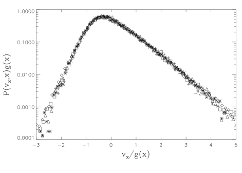
FIG. 8.: The scaling distribution $\phi(z)=P(v_{x},x)g(x)$. The data of Fig. 7 have been rescaled according to Eq. (17), so three sets of data are from various positions, $x=L/5(+),L/2(\ast),4L/5(\diamond)$, in a system with the usual energy enput at $x=0$. The plot also includes probability distributions from a simulation of a system that is identical to that used in Fig. 7 but with a different type of forcing at the heated wall. Data from this simulation is displayed for $x=7L/10(\triangle),4L/5(\Box)$.

IV Conclusion

In this work, we examined the steady-state behavior of a weakly inelastic two-dimensional driven granular system. We found that a hydrodynamic formulation provides a satisfactory description of the near-equilibrium behavior of the system in the quasi-elastic limit. We extended Haff’s theory to the low density limit and found that the corresponding temperature profile varies linearly in space. For slightly higher inelasticities, the system is no longer close to equilibrium in the low density limit. However, the scaling behavior of the velocity distributions suggests that a hydrodynamic treatment can still be useful in describing the system.

In this non-equilibrium regime, we found that the particle velocity distributions were non-Gaussian. Indeed, deviations from normal distributions have been observed in theoretical [10, 12, 13] and experimental studies[14]. In addition to this variation in the velocity distributions, systems of this sort can produce highly inhomogeneous spatial distributions, as has been noted elsewhere in one [4, 5] and two [7, 15] dimensions. A recent experimental study examined the spatial distribution of hard particles in two dimensions in the presence of an energy input [16]. Their data is in qualitative agreement with our theoretical predictions, and inhomogeneous spatial distributions reminiscent of Fig. (1) are observed.

Acknowledgements: We are indebted to Leo Kadanoff for stimulating our interest in this problem. We also thank Bill Young, Tom Witten, Sergei Esipov and Thorsten Pöschel for useful discussions. This work was supported by the National Science Foundation under Awards #DMR-9415604 and #DMR-9208527 and the MRSEC Program, Award #DMR-9400379.

FIG. 9.: Characteristic velocity scale as a function of position. Here we plot $\langle(v_{x}^{2}+v_{y}^{2})^{1/2}\rangle\propto g(x)$ (the dashed line). This data was obtained from the simulation used to make Fig. 7 and the values for $g(x)$ were used to do the rescaling in Fig. 8. We also plot $\langle v_{x}^{2}+v_{y}^{2}\rangle\propto g^{2}(x)$ (the solid line) to show that it is a roughly linear function of position, as predicted by Eq. (19).

REFERENCES

- [1] H. M. Jaeger, S. R. Nagel, and R. P. Behringer, Phys. Today 49, 32 (1996).
- [2] P. K. Haff, J. Fluid Mech. 134, 401 (1983).
- [3] J. T. Jenkins and M. W. Richman, J. Fluid Mech. 192, 313 (1988).
- [4] Y. Du, H. Li, and L. P. Kadanoff, Phys. Rev. Lett. 74, 1268 (1995).
- [5] E. L. Grossman and B. Roman, Phys. Fluids 8, 3218 (1996).
- [6] J. Maddox, Nature 374, 11 (1995).
- [7] S. E. Esipov and T. Pöschel, “Boltzmann equation and granular hydrodynamics,” preprint.
- [8] H. Hayakawa, S. Yue, and D. C. Hong, Phys. Rev. Lett. 75, 2328 (1995).
- [9] L. Tonks, Phys. Rev. 50, 955 (1936).
- [10] I. Goldhirsch and G. Zanetti, Phys. Rev. Lett. 70, 1619 (1993).
- [11] S. McNamara and W. R. Young, Phys. Rev. E 53, 5089 (1996).
- [12] Y. D. Lan and A. D. Rosato, Phys. Fluids 7, 1818 (1995).
- [13] Y. H. Taguchi and H. Takayasu, Europhys. Lett. 30, 499 (1995).
- [14] S. Warr, G. T. H. Jaques, and J. M. Huntley, Powder Tech. 81, 41 (1994).
- [15] S. McNamara and J.-L. Barrat, “The energy flux into a fluidized granular medium at a vibrating wall,” preprint.
- [16] A. Kudrolli, M. Wolpert, and J. P. Gollub, “Cluster formation due to collisions in granular material,” preprint.