Non-equilibrium Monte Carlo dynamics of the Sherrington-Kirkpatrick mean field spin glass model

Abstract

We present a numerical study of the non-equilibrium dynamics of the Sherrington-Kirkpatrick model. We analize the overlap distribution between the configurations visited at the time $t$ and in particular its scaling behaviour with the size of the system. We find two different non-equilibrium dynamical regimes. The first is a proper Out of Equilibrium Regime, that is the relevant regime for the dynamics of an infinite system. The second is an Intermediate Regime that separates the Out of Equilibrium Regime from equilibrium. After studying the crossover beetween the two regimes, we focus on the Out of Equilibrium Regime and we reveal some of the geometrical features of phase space. According to recent analitical work, we find that the asymptotic out of equilibrium energy density is the equilibrium one. The same happens to the staggered-magnetisation, suggesting there is a deep geometrical similarity between equilibrium and out of equilibrium configurations. A procedure, that we call clonation, shows that the dynamics follows sort of canyons, as opposed to a system of independent traps.

1 Introduction

In the last years, the experimental, numerical and theoretical interest on the non-equilibrium properties of spin glasses [1, 2, 3] has increased. Experiments have shown a very rich behaviour in many different materials (see for example [4, 5, 6, 7]). Some particular procedures have focused on measuring the main feature of the slow spin glass dynamics: the aging phenomena. Simulations carried out on tridimentional spin glass models [8] show some of the characteristics (slow dynamics, aging) seen in experiments, but suffer of a lack of a microscopic description. A recent analitical work [9] on the mean-field Sherrington-Kirkpatrick model (SK) contribute to fill this gap, and confirm that spin-glasses represent a ground for developing non-equilibrium statistical mechanics.

In the present work we study the Monte Carlo heath-bath dynamics (with Metropolis sequential updating algorithm) of the SK model [10], defined by the Hamiltonian:

$$H_{J}[\sigma]=-\frac{1}{2}\sum_{i\neq j}J_{ij}\sigma_{i}\sigma_{j}$$ (1)

The $J_{ij}$ are random Gaussian variables with variance $1/\sqrt{N}$.

We test some recent analitical predictions [9, 11], and get insight into the geometrical properties of the phase space interested by the dynamics. For this aim we use the technique of dynamics clonation [12, 13, 14] that though experimentally unimplementable, is easy to implement numerically and give us insight in the nature of the dynamics.

One of the main purposes of this paper is to study the range of validity of the analytical solution obtained in the thermodynamical limit ($N\rightarrow\infty$) when the size of the system is finite ($N$ finite). We find the ($N$,$t$) scalings to have a mean-field like Out of Equilibrium regime, an Intermediate regime and the final Equilibrium regime.

This paper is organized as follows: In Section II we present the definitions of various quantities we study in this paper and we discuss different limiting procedures leading to equilibrium or out of equilibrium dynamics. Section III is devoted to the numerical results. Finally in Section IV we present our conclusions.

2 General Considerations

Before reporting the results of the simulations, let us observe that during a simulation the measured quantity $O$ always depends on the size of the system (the number of spins $N$) and on time (the number of Monte Carlo sweeps preceeding the measuring time $t$). In the following we shall show this dependency explicitly: $O(N,t)$. The equilibrium value is given by the Asymptotic Limit (AL) $lim_{t\rightarrow\infty}O(N,t)=O(N)$. The thermodynamical analytical calculations give the equilibrium value for an infinite system, that is the Thermodynamical Limit (TL) of the equilibrium quantity: $\lim_{N\rightarrow\infty}O(N)=O_{eq}$. So, if we are interested in the equilibrium properties of the system we have to consider the following ordered limit procedure:

$$\lim_{N\rightarrow\infty}\lim_{t\rightarrow\infty}O(N,t)=\lim_{N\rightarrow\infty}O(N)=O_{eq}$$

Now let us consider the opposite order of the limits. If the system undergoes a phase transition, the TL can break the ergodicity of the phase space. In such a case, the AL of the TL may be different from the equilibrium thermodynamical value:

$$\lim_{t\rightarrow\infty}\lim_{N\rightarrow\infty}O(N,t)=\lim_{t\rightarrow\infty}O(t)=O_{o.eq}\neq O_{eq}$$

Some recent analytical works [15, 9] deal with this opposite ordered limit procedure to describe the out of equilibrium properties of spin glasses. We call the asymptotic dynamics of an infinite system, in the sense of this order of limits, the non-equilibrium dynamics.

In a real simulation, we cannot perform neither AL nor the TL. We consider systems of growing size, and for each one we consider an equilibration time after which the system is equilibrated. The correct criterion for choosing the equilibration time is not so trivial, especially for systems like spin-glasses, that evolve extremely slowly as shown clearly by experiments. We can consider the spin-glass model equilibrated when the Two-Times Quantities 2TQ do not depend explicitly upon both times, but only upon the time difference (for brevity Homogeneous Time Dependence). For example if we consider the Two-Times Auto-Correlation Function

$$C_{N}(t,t^{\prime})=\overline{<1/N\sum_{i=1,N}\sigma_{i}(t)\sigma_{i}(t^{\prime})>}$$ (2)

we are sure that the system forgot the initial $t=0$ randomly chosen configuration only when $C_{N}(t,t^{\prime})=C_{N}(t-t^{\prime})$. Hereafter we follow the standard motation, indicating the thermal average (different noise realization, but fixed $J_{ij}$) with $<\bullet>$, and the sample average (different chosen $J_{ij}$) with $\overline{\bullet}$.

Unfortunately, the measurements of 2TQ are very computer time consuming, because we have to keep track of all previous configurations of the system. It would then be better use an equilibration criterion involving only One-Time Quantities 1TQ. However, in a glassy system, a 1TQ may reach the definitive asymptotic value, very near or equal to the equilibrium value, even when the system is very far from equilibrium and, for example, the Auto-Correlation Function (2) is far from being Homogeneous in times. So just checking for the asymptotic value of a 1TQ can lead to erroneous results.

3 Numerical Simulations

3.1 The Overlap as the geometrical Clock

It is well known [1] that the SK model (1) undergoes a phase transition at $T_{c}=1$. The order parameter is the Parisi $q(x)$ function that is related to the overlap distribution function of the equilibrium states $P(q)$: $P(q)=(\frac{dq}{dx})^{-1}$ (For a recent numerical analysis, see [16]). To monitor the order parameter, $q(x)$, we measure the first non-zero momentum of the $P(q)$ overlap distribution, that in the zero field case is:

$$q_{2}(N,t)=\overline{<[(1/N)\sum_{i=1,N}\sigma_{i}(t)\tau_{i}(t)]^{2}>}$$ (3)

i.e. the second momentum. Here $\sigma_{i}(t)$ and $\tau_{i}(t)$ denote the configuration at time $t$ of two realization of the dynamics ($J_{ij}$ fixed), with independent randomly chosen initial configurations and independent noise realization. Hereafter we shall call them replicas.

The quantity $q_{2}$ is used to determine the equilibration of the SK model for example in [17]. They use the relation $q_{2}=1-2TE$ [18] (where $E=\lim_{N\rightarrow\infty}\lim_{t\rightarrow\infty}[\overline{<H>}/N]$ is the equilibrium energy density) to determine the times $t<t_{0}$ to skip before attempting the equilibrium measure. On the contrary, in this work we are interested in the evolution before the equilibration.

We check explicitly the hypothesis that $q_{2}$ represents a good “clock” for the dynamics, as shown in Fig.1. We concentrate much of our efforts studing this quantity before it reaches the equilibrium value and in particular its scaling behaviour respect to the size of the system.

Figure 1: The Auto-Correlation Functions (2) become time-homogeneous only when $q_{2}(N,t)$ (3) reaches its equilibrium value. In (A) the system is equilibrated, in (B) the system is out-of-equilibrium (the equilibrium value of $q_{2}(N,t)$ is greater then $0.3$). The data refer to 200 different samples (i.e. 200 different chosen $\{J_{i,j}\}$). For each sample we use at least 10 replicas (see text) to measure $q_{2}(N,t)$.

We simulate the dynamics of $q_{2}(N,t)$ for several system sizes at fixed temperature. The value of $q_{2}(N,t=0)$ is generally $1/N$, because the starting configuration for each replica is choosen randomly and independently. A different choice for the starting value of $q_{2}$ is not determinant for the subsequent dynamics, apart from approximately the first hundred steps.

The dynamics of $q_{2}(N,t)$ is characterized by a monotonic growth towards the equilibrium value. We identify two non-equilibrium regimes, characterized by different scaling properties respect to the size of the system.

• Out of Equilibrium Regime.

  In the first regime, $q_{2}(N,t)$ scales as $1/N$, with the law

  $$q_{2}(N,t)\propto(1/N)\ln(t)$$

  In Fig.2 we show the universal quantity $Nq_{2}(N,t)$ vs. $t$ for systems of different size. The temperature dependence is restricted to the proportionality constant. We call this regime the Out of Equilibrium Regime. In the gedanken-simulation of an infinite system $q_{2}(t)$ would be constantly zero.

  

  Figure 2: The “clock” $q_{2}(N,t)$ in the Out of Equilibrium Regime multiplicated by $N$ for systems of different size. The data refer to a minimum of 10 replicas for each of 200 samples.

• Intermediate Regime.

  As the $q_{2}(N,t)$ reaches a sensible fraction of its equilibrium value, the scaling behaviour changes. We tried a fit for this scaling. For a fixed temperature, we plot the quantity $q_{2}(N,t)/q_{2}^{eq}(N)$ vs. $\ln(t)/N^{\alpha}$. Varying $\alpha$, we looked for the collapse of the curves associated to systems of different size. In Fig.3 is shown the result for $T=0.4T_{c}$, that indicates a value $\alpha\approx 0.5$. But the value of $\alpha$ is temperature dependent. For different temperatures we found values in the range between $1$ and $1/3$. We called this regime the Intermediate Regime.

  

  Figure 3: In the Intermediate Regime $q_{2}(N,t)$ scales as $1/N^{\alpha}$. Here we plot $q_{2}(N,t)$ vs. $\ln(t)/N^{\alpha}$ for the value $\alpha=0.5$, the more appropriate for this temperature ($T=0.4T_{c}$).

The cross-over between the two regimes is shown in Fig.4. We plot the quantity $Nq_{2}(N,t)$ that follows an universal curve (at fixed temperature) in the first regime. Larger systems depart from this curve later, since the cross-over time grows with the system size. We define the cross-over time as the time before the difference between the $Nq_{2}(N,t)$ and the universal curve $\lim_{N\rightarrow\infty}Nq_{2}(N,t)$ reaches a fixed tollerance value. In Fig.5 we show the cross-over time vs. the size of the system. We guess a linear behaviour.

Figure 4: Cross-over from the Out of Equilibrium regime to the Intermediate regime. The plot represents the quantity $Nq_{2}(N,t)$ vs $t$ for several systems of growing size. Note that the curves assciated to $N=640$ and $N=1280$ collapse, indicating that the two systems are still both in the Out of Equilibrium Regime for the whole time window. The curve for $N=1280$ has been used as the limiting curve for the determination of the Cross-Over time.

Figure 5: Cross-Over time between the two non-equilibrium regimes vs the size of the system $N$. The fit suggests a linear behaviour.

In Fig.6 we show the response of the dynamical “clock” $q_{2}(N,T)$ to a “positive” cycle of temperature. We rise the temperature to a still subcritical value for a period, after that we restore it to the initial value. The overall effect of the cycling procedure is that the system goes closer to the equilibrium, since the $q_{2}(N,t)$ “clock” reaches a higher value than the one obtained, at the same time, in the absence of the temperature cycle.

Such behaviour seems different from the experimental results reported by Hamman et al. in [6], where they see, for positive temperature cycles, a restart of the dynamics, i.e. a loose of memory of the evolution before the heat pulse.

However let us note that the response of the system to the positive increase of the temperature is very different from the response to the decrease.

Figure 6: Response of the “clock” of the dynamics $q_{2}(N,t)$ to a cycle of temperature. In the inset we show the temperature vs the time $t$. We have performed a short heat pulse.

3.2 Out of Equilibrium Regime

As we are interested in the out-of-equilibrium dynamics of the model, in the sense of the ordered limit procedure AL after TL, we study the dynamics of some quantities in the first dynamical regime, i.e. the Out of Equilibrium Regime.

The Energy density of the system at time $t$ is:

$$E(N,t)=(1/N)\overline{<H(t)>}$$ (4)

The relaxational dynamics of the Energy density for the SK model has been extensively studied (for example in [19]). Here we want to focus into its asymptotic value. To this aim, we reparametrize the energy density curve with respect to the dynamical “clock” $q_{2}(N,t)$, that indicates the equilibration level of the system at time $t$.

The Figure 7 shows the result of such reparametrization. The line is the equilibrium relation $E=-\beta/2(1-q_{2})$. The first two curves refer to systems that reach equilibrium at the end of the simulation. The others, with growing size, are farther from equilibrium, but closer to the energy density equilibrium value. A plausible proposal for the limiting curve associated to an infinite system is a step function that, starting from $E=0$, $q_{2}=0$, abruptely collapses to the constant value $E=E_{eq}$ for $q_{2}>0$. Besides it means that this 1TQ does not represent a good choice for the determination of the equilibration time.

Our results disagree with those by Scharnagl et al. in [20]. The results of their power law fit on the first 130 steps for the energy dynamics of an infinite system (they use an interesting new procedure to simulate the dynamics of infinite sized systems [21]) indicate an asymptotic energy value $e_{\infty}$ different from the equilibrium value for temperature below $0.5T_{c}$.

On the contrary, we find that the system relaxes to its equilibrium energy density. To corroborate our result, we summarize here previously published results [11].

Figure 7: Energy density relaxation curve in function of the corresponding value of the “clock”, i.e. $E(N,t)$ vs $q_{2}(N,t)$.

Consider $\sigma_{\lambda}$ the projection of the configuration vector $\overrightarrow{\sigma}(t)=\{\sigma_{i}(t)\}$ on the set of eigen-vectors $\overrightarrow{J}(\lambda)$ of the coupling matrix $\{J_{ij}\}$. We measure the so called staggered magnetisation, i.e.

$$g_{N,t}(\lambda)=\overline{<(\sigma_{\lambda}(t))^{2}>}$$

where $\sigma_{\lambda}(t)=\sum_{i=1,N}\lambda_{i}\sigma_{i}(t)$, $\{\lambda_{i}\}$ being the coordinates of the $\hat{\lambda}$-eigenvector of the coupling matrix ($\sum_{j=1,N}J_{i,j}\lambda_{j}=\hat{\lambda}\lambda_{i}$).

The staggered magnetization is a distribution that contains a lot of informations. In particular its first momentum is the energy density (4), object of our previous discussion. More precisely:

$$\lim_{N\rightarrow\infty}E(N,t)=-\lim_{N\rightarrow\infty}\int_{-2}^{2}\lambda\rho(\lambda)g_{N,t}(\lambda)d\lambda$$

where $\rho(\lambda)$ is the well known semicircle distribution for the eigenvalue of the $J_{ij}$ random matrix [22].

In Fig.8 we show the staggered-magnetization, multiplicated by the eigenvalue semicircle distribution $\rho(\lambda)$, compared with the equilibrium curve [23]. We note a very fast convergence of the out of equilibrium staggered magnetization to the equilibrium curve, when the system is still very far from equilibrium (as revealed by the $P(q)$ shown in the figure inset).

Figure 8: Staggered magnetisation calculated at different non-equilibrium times (from ref. [11]). In the inset we show the overlap distribution for the same times. The full lines correspond to the prediction of the replica ansatz for the equilibrium.

The Auto-Correlation function (2) shows aging behaviour (see Fig.9), confirming the weak ergodicity breaking hypothesis ([24],[9]):

$$\lim_{\tau\rightarrow\infty}C(t_{w},t_{w}+\tau) =0$$

$$\frac{\partial C(t_{w},t_{w}+\tau)}{\partial\tau} \leq 0 \forall\textnormal{(fixed)}t_{w}$$

$$\frac{\partial C(t_{w},t)}{\partial t_{w}} \geq 0 \forall\textnormal{(fixed)}t>t_{w}$$

Figure 9: Auto-correlation functions $C(t_{w},t_{w}+\tau)$ vs $\tau/t_{w}$ for different $t_{w}$. We do not note a simple $\tau/t_{w}$ behaviour.

Consider the fluctuations of the Auto-Correlation Functions:

$$F_{N}(t,t^{\prime})=\overline{<(1/N\sum_{i=1,N}\sigma_{i}(t)\sigma_{i}(t^{\prime})-C_{N}(t,t^{\prime}))^{2}>}$$ (5)

In the equilibrium case the fluctuations have a finite, extensive and not self-averaging value (see [17]):

$$\lim_{N\rightarrow\infty}\lim_{t_{w}\rightarrow\infty}F_{N}(t_{w},t_{w}+\tau)=q_{2}-q_{1}^{2}$$

where $q_{n}=\int{q^{n}P(q)dq}$ is the n-th momentum of the equilibrium order parameter P(q).

Instead, in the Out of Equilibrium Regime such quantities scale to zero with the size of the system. To show this, we have integrated the fluctuations for several sized systems. In Fig.10 we show the results for different values of $t_{w}$. We fit each curve with a power law $F_{N}\propto N^{a}$ (the result is shown in the legend).

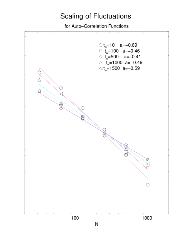
Figure 10: Scaling of Auto-correlation Fluctuations

3.3 Clonation Procedures

To obtain a clearer picture of the geometrical landscape, where the out of equilibrium dynamics take place, we perform a particular simulation procedure that we call “clonation” [12, 13, 14]. Since we are interested in the phace space region visited by the dynamics after a certain time $t_{w}$, we proceed to let evolve a single system with the usual Monte Carlo dynamics, until such a time. At $t_{w}$ we create a number of copy of this system, i.e. systems exactly in the same configuration (we clone it). Subsequently we let them (the original and the clones) evolve independently, that is to say with the same Hamiltonian, but different noise realizations.

These systems represent different possible histories of the first system, as if it had met, in its Monte Carlo dynamics, a different random number sequence after the time $t_{w}$. There is a difference between these copies (clones) of the system and the previously defined replicas. The replicas start at time $t=0$ from independently choosen configurations and evolve with independent dynamics (same Hamiltonian, different noises). We may think at the clones like starting from the same configuration at the time $t=0$ and evolving identically (same Hamiltonian and same noise) until the time $t=t_{w}$ (obviously this process is not actually simulated).

This clonation procedure is different from a damage spreading procedure (see for example [25, 26]), where two systems starting at measured distance evolve whith the same noise. The damage spreading procedure was used to individuate temperatures which could be compared with equilibrium and dynamical transition temperatures.

Our aim here is to investigate the geometry of the phase space monitoring the Auto-Correlation Function (2), and the Clones-Correlation Function, defined by:

$$Q_{(N,t_{w})}(t)=\overline{<1/N\sum_{i=1,N}(\sigma_{i}(t)\tau_{i}(t))>}$$ (6)

($\sigma$ e $\tau$ are the spins of two different clones).

These quantities are simply related to the Euclidean distance in phase space. The Auto-Correlation (2) is related to the Euclidean distance between the configuration of each clone at the time $t_{w}$ with its own configuration at the time $t>t_{w}$ as:

$$\overline{<\frac{1}{N}\sum_{i=1,N}(\sigma_{i}(t_{w})-\sigma_{i}(t))^{2}>}=2(1-C_{N}(t_{w},t))$$

Similarly the Clones-Correlation (6) is related to the distance between the clones (generated at the time $t_{w}$) at the time $t$:

$$\overline{<\frac{1}{N}\sum_{i=1,N}(\sigma_{i}(t)-\tau_{i}(t))^{2}>}=2(1-Q_{(N,t_{w})}(t))$$

In Fig.11 we show the results of the measurement. We see that at first we have $C>Q$, but, after some time, this relation inverts, and we have $Q>C$.

Remembering the relations of these quantities with the euclidean distances, it means that at first the clones go away from each others more than how much they drift away from the initial configuration at the time $t_{w}$. But after, they continue their drift standing close and forgetting the initial $t_{w}$ configuration. The simplest picture representing such a behaviour is that of a dynamics following canyons or in corridors: at first the clones span the width of the channel and, after, they drift away along it.

If the situation has been that of a series of independent traps (like for example in [24]) we should see a different behaviour, probably with $Q=C$. Here we see, at least, a kind of hierarchy of traps [27].

In the present work we do not get the asymptotic limit of $Q$. We suspect that it goes to zero, even if the curve is very slow but we can not exclude that it may reach a costant value different from zero.

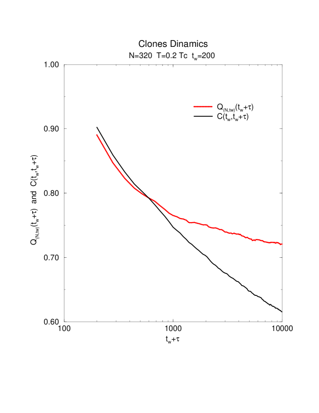
Figure 11: Clonation of the system at the time $t_{w}$. the plot shows the Auto-Correlation (2) and the Clones-Correlation (6).

4 Conclusions

The non-equilibrium dynamics of the SK model takes place in a range of time that grows exponentially with the size of the system. In this region, we identify two distinct regimes, characterized by different scaling properties of $q_{2}(N,t)$ the average squared overlap beetween two typical configurations visited at time $t$. The quantity $q_{2}(N,t)$, for a system in equilibrium, represents the second momentum of the $P(q)$ distribution, the order parameter for the phase transition. In the case of a large system that starts the dynamics from a random configuration, or that equivalently is abruptely cooled from high temperature to a subcritical one, the relevant regime is the first Out of Equilibrium Regime, during which the $q_{2}(N,t)$ scales to zero as $1/N$. In such a situation the dynamics is non-stationary, presenting generic aging properties and confirming a scenario of weak ergodicity breaking. As claimed by recent analitical works [15, 9, 11], the asymptotic configurations reached by an infinite SK model, present some similarities with the equilibrium distribution: the out of equilibrium staggered magnetisation equals the equilibrium one and so does the energy density [11]. But the configurations visited are not real equilibrium configurations and the system allways escapes from them, never to return. These configurations present a sort of hierarchical structure. A special clonation procedure shows that the dynamics takes place following corridors or canyons and that phace space looks like a kind of fast flat labyrinth that the system explores always slower looking for the equilibrium configurations. Such a simple numerical procedure reveals that the spin-glass dynamics is not simply a two-well energy problem, but we have to consider more complex situations (see for example [28] or [29])

References

- [1] M. Mezard, G. Parisi, and M. A. Virasoro. Spin Glass Theory and Beyond. World scientific, Singapore, 1986.
- [2] K. Binder and A.P. Young. Spin glasses: Experimental facts, theoretical concepts, and open questions. Rev. Mod. Phys., 58(4):801–976, October 1986.
- [3] K.H. Fischer and J.A. Hertz. Spin glasses. Cambridge University Press, 1991.
- [4] L. C. E. Struik. Physical aging in amorphous polymers and other materials. Elsevier, Houston, 1978.
- [5] L. Lundgren. Experiments on spin glass dynamics. In I. A. Campbell and C. Giovannella, editors, Relaxation in Complex Systems and Related Topics, New York, 1990. Plenum Press.
- [6] E. Vincent, J.Hamman, and M.Ocio. In D. H. Ryan, editor, Recent progress in random magnets, Singapore, 1987. World Scientific.
- [7] E. Vincent, J.Hamman, M.Ocio, J. P. Bouchaud, and L. F. Cugliandolo. Slow dynamics and aging in spin glasses. In M.Rubi, editor, Complex behaviour in glassy systems. Springer Verlag, in press.
- [8] H. Rieger. Monte Carlo Studies of Ising Spin Glasses and Random Field Systems. In D. Stauffer, editor, Annual Reviews of Computational Physics, volume II, Singapore, 1995. World Scientific.
- [9] L. F. Cugliandolo and J. Kurchan. On the Out of Equilibrium Relaxation of the Sherrington-Kirkpatrick model. J. Phys., A(27):5749, 1994.
- [10] D. Sherrington and S. Kirkpatrick. Solvable Model of a Spin Glass. Phys. Rev. Lett., (35):1792, 1975.
- [11] A. Baldassarri, L. F. Cugliandolo, J. Kurchan, and G. Parisi. On the out of equilibrium order parameter in long-range spin-glasses. J. Phys., A(28):1831, 1995.
- [12] Andrea Baldassarri. Studio della dianamica fuori dall’equilibrio di un modello di vetro di spin in campo medio. Universitá degli studi di Roma “La Sapienza”, March 1995. Tesi di laurea.
- [13] L. F. Cugliandolo and D. S. Dean. J. Phys., A(28):4213, 1995.
- [14] A. Barrat, R. Burioni, and M. Mezard. Aging classification in glassy dynamics. J. Phys.A, 29(7):1311–1330, 1996.
- [15] L. F. Cugliandolo and J. Kurchan. Analitycal Solution of the Off-equilibrium Dynamics of a Long Range Spin-Glass Model. Phys. Rev. Lett., (71):1, 1993.
- [16] M. Picco and F. Ritort. Numerical study of the Ising spin glass in a magnetic field. J. Phys. I (France), (4):1819, 1994.
- [17] N. D. Mackenzie and A. P. Young. Statics and dynamics of the infinite-range Ising spin glass model. J. Phys., C(16):5321, 1983.
- [18] A. J. Bray and M. A. More. J. Phys., C(13):419, 1980.
- [19] W. Kinzel. Remanent magnetization of the infinite-range Ising spin glass. Phys. Rev., B(33):7, 1986.
- [20] Andrea Scharnagl, Manfred Opper, and Wolfgang Kinzel. On the relaxation of infinite-range spin glasses. J. Phys., A(28):5721, 1995.
- [21] H. Eisfeller and M. Opper. New Method for Studying the Dynamics of Disordered Spin Systems without Finite-Size Effects. Phys. Rev. Lett., (68):2094, 1992.
- [22] M. L. Mehta. Random matrices and the statistical theory of energy levels. Academic, New York/London, 1967.
- [23] M. Mezard and G. Parisi. Self-averaging correlation functions in the mean field theory of spin glasses. J. Physique Lett., (45):L–707, 1984.
- [24] J. P. Bouchaud. Weak ergocidity breaking and aging in disordered systems. J. Physique, I (France)(2):1705, 1992.
- [25] B. Derrida. Dynamical phase transitions and spin glasses. Physics Reports, 184(2-4):207–212, 1989.
- [26] I.A. Campbell and L. de Arcangelis. On the damage spreading in ising spin glasses. Physica, A(178):29, 1991.
- [27] J. P. Bouchaud and D. S. Dean. Aging on Parisi’s tree. J. Physique, I (France)(5):265, 1995.
- [28] J. Kurchan and Laurent Laloux. Phace space geometry and slow dynamics. J. Phys., A(29):1929, 1996.
- [29] F. Ritort. Glassiness in a Model without energy barriers. Phys. Rev. Lett., (75):1190, 1995.