Mesoscopic conductance fluctuations in dirty quantum dots with single channel leads

Abstract

We consider a distribution of conductance fluctuations in quantum dots with single channel leads and continuous level spectra and we demonstrate that it has a distinctly non-Gaussian shape and strong dependence on time-reversal symmetry, in contrast to an almost Gaussian distribution of conductances in a disordered metallic sample connected to a reservoir by broad multi-channel leads. In the absence of time-reversal symmetry, our results obtained within the diagrammatic approach coincide with those derived within non-perturbative techniques. In addition, we show that the distribution has lognormal tails for weak disorder, similar to the case of broad leads, and that it becomes almost lognormal as the amount of disorder is increased towards the Anderson transition.

Recently it has been shown that the conductance of clean quantum dots with point-like external contacts (lead width $w\approx\hbar k_{F}^{-1}$, where $\hbar k_{F}^{-1}$ is the Fermi wavelength) have non-Gaussian distribution functions [1, 2]. Weak transmission through the contacts means that the electrons typically spend more time in the system than that required to cross it so that the energy level broadening due to inelastic processes in the dot $\gamma\ll E_{c}$ where $E_{c}\approx\hbar D/L^{2}$ is the Thouless energy. This inequality corresponds to the zero mode regime which allows the use of non-perturbative techniques including random matrix theory [3] and the zero dimensional supersymmetric $\sigma$ model [4]. In contrast, it is known that the distribution function of the conductance is mainly Gaussian [5] in a weakly disordered open sample connected to a reservoir by broad external contacts of width $w>\ell$, where $\ell$ is the elastic mean free path. Inelastic scattering processes in the reservoir result in a level broadening $\gamma\sim E_{c}$.

In the present paper the aim is to determine the distribution function of a dirty quantum dot with two point contacts (which allow a single transport channel). We will describe the regime of continuous energy levels, $\gamma\gtrsim\Delta$, where $\gamma$ is the broadening due to inelastic scattering in the dot and $\Delta$ is the mean level spacing. This overlaps with the supersymmetric (SUSY) calculations [1] in the ergodic regime, $\Delta\lesssim\gamma<E_{c}$. While the SUSY approach is valid also in the quantum regime, $\gamma<\Delta$, a perturbative diagrammatic approach applied below can be used also for $\gamma\gtrsim E_{c}$. In this case all diffusion modes contribute to the conductance rather than a single homogeneous “zero” mode which is the only mode taken into account within the nonperturbative SUSY calculations. The conductance distribution function has a non-Gaussian shape also for such a strong level broadening so that the non-Gaussian shape is due to geometric factors – namely, the point-like structure of contacts, rather than due to the dominance of the zero mode. In addition, we will use a standard renormalisation group technique to consider the rôle of increasing disorder in the dot.

Traditionally the conductance of a system with broad, spatially homogeneous contacts is considered by means of the Kubo formula [6]. For a lead geometry which involves spatially inhomogeneous currents, however, the conductance is often more conveniently expressed via scattering probabilities using the Landauer-Büttiker formula [7]. In this paper, we start by writing the conductance in terms of Green’s functions with the help of the Landauer-Büttiker formula. Then we will determine the conductance distribution in the case of a continuous energy levels spectrum, $\gamma\gtrsim\Delta$, finding the moments of conductance by diagrammatic perturbation expansion in the parameter $(\gamma/\Delta)^{-1}$. Finally we will use an effective functional of the non-linear $\sigma$ model as a framework for the renormalisation group analysis necessary to describe dependence of the moments of conductance (and thus of the distribution) on the disorder parameter. Following Ref. [5], we show that the $n$th order moments are proportional for large $n$ to exp$(un^{2})$ ($u$ is a certain parameter to be specified later) which is characteristic of a distribution function having lognormal tails. As the amount of disorder is increased towards the Anderson transition, the conductance distribution in the dot becomes almost entirely lognormal. Again, this is different from the conductance distribution in the ensemble of samples with broad leads which is also characterised by lognormal tails whose rôle is increasing with disorder, but remains mainly Gaussian within the whole range of validity of the renormalisation group analysis, even at the threshold of the transition.

We consider weak coupling through the contacts from the disordered region to electron reservoirs and we label probabilities for tunnelling through the contacts as $\alpha_{1}$ and $\alpha_{2}$ which are assumed to be constant. Following [1] the level broadening due to inelastic scattering $\alpha$ (in units of the mean level spacing $\Delta$) is chosen for convenience to be greater than $\alpha_{1}$ and $\alpha_{2}$. So we can write $\alpha=2\pi^{2}\gamma/\Delta$ where $\gamma$ is the total level broadening. We will present a perturbative calculation both in the many mode regime, $\gamma\gtrsim E_{c}$, where the relevant small parameter is $g^{-1}=(2\pi^{2}E_{c}/\Delta)^{-1}$ ($g$ is the average conductance of an open sample in units of $e^{2}/\pi h$) and in the zero mode regime, $\Delta\lesssim\gamma<E_{c}$, where the relevant small parameter is $\alpha^{-1}$. The calculation is not valid in the region $\alpha<1$ which was the main area of interest for previous zero mode calculations [1, 2]. Since we are modelling a disordered sample, and $\alpha\gtrsim 1$ (the level spectrum is continuous), we do not include Coulomb blockade and electron-electron interaction effects. As a result, the calculations are applicable to a disordered sample whose electronic charging energy is negligible compared to the Thouless energy (i.e. with spatial dimensions larger than usual quantum dots). However the calculations are also applicable to quantum dots when the gate voltage is such that the addition of a single electron does not change the total energy, conduction occurs and disorder effects are relevant [8]. Note that a similar non-Gaussian distribution of Coulomb blockade peak height fluctuations was found by Jalabert et al [9], and recent experiments [10] appear to be consistent with this prediction.

The framework for determination of the conductance is the Landauer-Büttiker formula [7]. We use it in the following form [11]:

$$G={e^{2}\over{2h}}\sum_{ab}\left(T_{ab}^{L}+T_{ab}^{R}\right),$$ (1)

where the transmission coefficient $T_{ab}^{L(R)}$ is the probability of transmission from the channel labelled by $a$ in the left (right) lead to the channel labelled by $b$ in the right (left) lead. The conductance has been written explicitly in terms of transmission from the left and from the right since this most symmetric form is required to consider the influence of broken time reversal symmetry on the fluctuations of the conductance. The transmission coefficients may be related to Green’s functions by [11, 12]

$$T_{ab}^{L(R)}=\frac{1}{(h\nu_{0})^{2}}{\cal G}^{+(-)}\left({\bf r_{1}},{\bf r_{2}};\varepsilon\right){\cal G}^{-(+)}({\bf r_{2}},{\bf r_{1}};\varepsilon),$$ (2)

where ${\cal G}^{+}$ (${\cal G}^{-}$) is a retarded (advanced) Green’s function and ${\bf r_{1}}$, ${\bf r_{2}}$ are the positions of the point contacts. In the entire energy interval of interest, $\varepsilon-\varepsilon_{F}\lesssim\hbar/\tau$, the mean density of states $\nu_{0}$ is a constant and the $T_{ab}^{L(R)}$ are energy independent so we will subsequently drop the $\varepsilon$ label ($\tau=\ell/v_{F}$ is the elastic scattering time).

Each point contact has a width $w\approx\hbar k_{F}^{-1}$ which corresponds to a single channel only so that the point to point conductance, $G$, is obtained from the Landauer-Büttiker formula, Eq. (1), with only one term in the summation. Ensemble averaged cumulants of the conductance, $\langle{\langle G^{n}\rangle}\rangle$, are given by

$$\langle{\langle G^{n}\rangle}\rangle=\left[{e^{2}\over{h}}{\alpha_{1}\alpha_{2}\over{(h\nu_{0})^{2}}}\right]^{n}\langle{\langle\left[{\cal G}^{+}\left({\bf r_{1}},{\bf r_{2}}\right){\cal G}^{-}\left({\bf r_{2}},{\bf r_{1}}\right)+{\cal G}^{+}\left({\bf r_{2}},{\bf r_{1}}\right){\cal G}^{-}\left({\bf r_{1}},{\bf r_{2}}\right)\right]^{n}\rangle}\rangle.$$ (3)

We consider the point contacts to be separated by a distance greater than the mean free path so that $|{{\bf r_{1}}-{\bf r_{2}}}|\gg\ell$. In Eq. (3) spin is explicitly included with an extra prefactor of $2$ and the term $\alpha_{1}\alpha_{2}$ represents the transmission probability through the contacts themselves. Ensemble averaging in Eq. (3) is performed within the impurity diagram technique [13] and it is convenient to use a representation in which slow diffusion modes are explicitly separated from fast “ballistic” ones [14]. Fig. 1b shows the dominant contribution to the mean conductance which contains one diffusion propagator (drawn as a wavy line which corresponds to a ladder series in the conventional technique [13]). At each end of the diffusion propagator there are two-sided ‘petal’ shapes which represent motion at ballistic scales since the average Green’s functions $\langle{\cal G}^{R,A}({\bf r},{\bf r^{\prime}})\rangle$ (drawn as edges of the petal) decay like $\exp(-|{\bf r}-{\bf r^{\prime}}|/2\ell)$. At the diffusive scale, $R\gtrsim\ell$, the petals reduce to the constant $\chi_{2}=2\pi\nu_{0}\tau$. The choice of diagrams is dictated by the inequality $|{\bf r_{1}}-{\bf r_{2}}|\gg\ell$. It means that a diagram with external points ${\bf{r_{1}}}$ and ${\bf{r_{2}}}$ connected solely by average Green’s functions as in Fig. 1a is exponentially small.

The diffusion propagator $D({\bf r},{\bf r^{\prime}};\omega)$ can be represented at zero frequency as

$$D({\bf r},{\bf r^{\prime}};0)=\frac{1}{2\pi\nu_{0}L^{d}\tau^{2}}\sum_{{\bf q}}\frac{1}{Dq^{2}+\gamma}\exp[i{\bf q}.({\bf r}-{\bf r^{\prime}})]\equiv\frac{1}{2\tau^{2}}\zeta(R),$$ (4)

where $D=v_{F}^{2}\tau/d$ is the diffusion constant and, for a closed system, the summation is carried out over all $\mathchoice{{\hbox{\boldmath$\displaystyle q$}}}{{\hbox{\boldmath$\textstyle q$}}}{{\hbox{\boldmath$\scriptstyle q$}}}{{\hbox{\boldmath$\scriptscriptstyle q$}}}=\pi\mathchoice{{\hbox{\boldmath$\displaystyle n$}}}{{\hbox{\boldmath$\textstyle n$}}}{{\hbox{\boldmath$\scriptstyle n$}}}{{\hbox{\boldmath$\scriptscriptstyle n$}}}/L$, where $\mathchoice{{\hbox{\boldmath$\displaystyle n$}}}{{\hbox{\boldmath$\textstyle n$}}}{{\hbox{\boldmath$\scriptstyle n$}}}{{\hbox{\boldmath$\scriptscriptstyle n$}}}=(n_{1},\ldots,n_{d})$ are non-negative integers. In an open system inelastic scattering occurs in the leads and the summation is cut off at low momenta $q\sim L^{-1}$ where $L$ is the system size. For the system with point contacts the energy level broadening, $\gamma$, due to inelastic processes inside the dot is inserted ‘by hands’ into Eq. (4). As a result, in the many mode regime, $\gamma\gtrsim E_{c}$, the summation in Eq. (4) may be approximated by an integration with cutoff at $q\sim L_{in}^{-1}$ where the inelastic scattering length $L_{in}=(D/\gamma)^{1/2}$. This leads to

$$\zeta(R)=\frac{2}{(4\pi)^{d/2}\pi\nu_{0}D}\left(\frac{2}{RL_{in}}\right)^{\epsilon/2}K_{\epsilon/2}(R/L_{in})\approx\cases{g_{0}^{-1}\ln(L_{in}/R),&$d=2$\cr(\pi/2g_{0})\,(\ell/R),&$d=3$}.$$ (6)

where $R=|{\bf r}-{\bf r^{\prime}}|$, $g_{0}\sim(\varepsilon_{F}\tau)^{d-1}$ is the dimensionless conductance of an open cube of size $\ell$, $d=2+\epsilon$ is the dimensionality of the dot, and $K_{\alpha}$ is the modified Bessel function of the third kind of order $\alpha$. In the zero mode regime, $\gamma\ll E_{c}$, the summation in Eq. (4) is dominated by the $q=0$ term so that

$$\zeta(R)\approx{2\pi\over{\alpha}},\qquad\alpha<E_{c}/\Delta,$$ (7)

which means that the diffusion propagator is independent of $R$, spatial dimensionality, and the degree of disorder.

Now the leading diagram for the mean conductance, shown in Fig. 1b, can be evaluated. Substituting $\chi_{2}=2\pi\nu_{0}\tau$ for the petals and $\zeta(R)$ for the diffusion propagator, one has

$$\langle G\rangle={e^{2}\over{h}}\alpha_{1}\alpha_{2}\,\zeta(R),$$ (8)

where $R\gg\ell$ is the separation of the point contacts. The mean conductance is proportional to $\zeta(R)$ and Eq. (7) shows that in the zero mode regime, $\gamma<E_{c}$, the mean conductance depends on the level broadening $\gamma$, but not on the separation of the point contacts, the dimensionality, or the degree of disorder. On the contrary, in the many mode regime, $\gamma\gtrsim E_{c}$, the mean conductance depends on all these parameters via Eq. (6); since it is inversely proportional to $g_{0}$ it actually increases as the amount of disorder increases.

In order to calculate the variance of the conductance, we consider the following correlation function between the transmission coefficient from the single channel at ${\bf r_{1}}$ to ${\bf r_{2}}$ and the transmission coefficient from the single channel at ${\bf{r_{1}}^{\prime}}$ to ${\bf{r_{2}}^{\prime}}$;

$$K(\Delta{\bf r_{1}},\Delta{\bf r_{2}})=2\left[{e^{2}\over{h}}{\alpha_{1}\alpha_{2}\over{(2\pi\nu_{0})^{2}}}\right]^{2}\langle{\langle{\cal G}^{+}\left({\bf r_{1}},{\bf r_{2}}\right){\cal G}^{-}\left({\bf r_{2}},{\bf r_{1}}\right){\cal G}^{+}\left({\bf{r_{1}}^{\prime}},{\bf{r_{2}}^{\prime}}\right){\cal G}^{-}\left({\bf{r_{2}}^{\prime}},{\bf{r_{1}}^{\prime}}\right)\rangle}\rangle.$$ (9)

We use the notation $\Delta{\bf r_{1}}={\bf r_{1}}-{\bf{r_{1}}^{\prime}}$, $\Delta{\bf r_{2}}={\bf r_{2}}-{\bf{r_{2}}^{\prime}}$, where $|\Delta{\bf r_{1}}|$, $|\Delta{\bf r_{2}}|\ll\ell$. The main contribution to $K$ is shown in Fig. 2a. It has two square “Hikami” boxes, $\chi_{4}$, representing motion at ballistic scales which are connected by two diffusion propagators, and it gives

$$K(\Delta{\bf r_{1}},\Delta{\bf r_{2}}) = 2\left[{e^{2}\over{h}}{\alpha_{1}\alpha_{2}\over{(2\pi\nu_{0})^{2}}}\right]^{2}\chi_{4}\!\left(\Delta{\bf r_{1}}\right)\,\chi_{4}\!\left(\Delta{\bf r_{2}}\right)\,\left[D\left({\bf r_{1}}-{\bf r_{2}}\right)\right]^{2},$$ (10)

$$\chi_{4}\!\left(\Delta{\bf r}\right) = \left|\int{\cal G}^{+}\left({\bf k}\right){\cal G}^{-}\left({\bf k}\right)e^{i{\bf k.\Delta{\bf r}}}\,d{\bf{k}}\right|^{2}.$$ (11)

To determine the behaviour of $K$ on length scales $|\Delta{\bf r_{1}}|$, $|\Delta{\bf r_{2}}|\ll\ell$ we need to evaluate $\chi_{4}\!\left(\Delta{\bf r}\right)$ accurately, rather than substituting it by const$\times\delta(\Delta{\bf r})$ which is sufficient for $|\Delta{\bf r}|\gg\ell$. We find that

$$\!\!\!\!\!\!\int{\cal G}^{+}\left({\bf k}\right){\cal G}^{-}\left({\bf k}\right)e^{i{\bf k.\Delta{\bf r}}}d{\bf{k}}$$ (12)

$$= \pi\nu_{0}\tau\left(\frac{\pi}{2{k_{{\!}_{F}}}\Delta r}\right)^{\epsilon/2}\!\left[H_{\epsilon/2}^{(1)}({k_{{\!}_{F}}}\Delta r\!+\!i\Delta r/2\ell)+H_{\epsilon/2}^{(2)}({k_{{\!}_{F}}}\Delta r\!-\!i\Delta r/2\ell)\right],$$ (13)

where $H_{\epsilon/2}^{(1,2)}$ are Hankel functions. In three dimensions this gives

$$K(\Delta{\bf r_{1}},\Delta{\bf r_{2}})={1\over 2}\left[{e^{2}\over{h}}\alpha_{1}\alpha_{2}\zeta(R)\right]^{2}\left[{\sin^{2}(k_{F}\Delta r_{1})\over(k_{F}\Delta r_{1})^{2}}{\sin^{2}(k_{F}\Delta r_{2})\over(k_{F}\Delta r_{2})^{2}}\,e^{-(\Delta r_{1}+\Delta r_{2})/\ell}\right],$$ (14)

which corresponds, in the limit $|\Delta{\bf r_{1}}|=0$, to the correlation function for optical speckle patterns found in [15].

We find from Eq. (13) that $\chi_{4}(0)=(2\pi\nu_{0}\tau)^{2}$ so that, in the single channel limit $|\Delta{\bf r_{1}}|=|\Delta{\bf r_{2}}|=0$, we get $K(0,0)=\langle G\rangle^{2}/2$. This corresponds to redrawing the diagram with the external points ${\bf{r_{1}}^{\prime}}$ and ${\bf{r_{2}}^{\prime}}$ exactly equal to ${\bf r_{1}}$ and ${\bf r_{2}}$, respectively, as shown in Fig. 2b. Note that although in each of the boxes in Fig. 2a $\mathchoice{{\hbox{\boldmath$\displaystyle r$}}}{{\hbox{\boldmath$\textstyle r$}}}{{\hbox{\boldmath$\scriptstyle r$}}}{{\hbox{\boldmath$\scriptscriptstyle r$}}}\approx\mathchoice{{\hbox{\boldmath$\displaystyle r$}}}{{\hbox{\boldmath$\textstyle r$}}}{{\hbox{\boldmath$\scriptstyle r$}}}{{\hbox{\boldmath$\scriptscriptstyle r$}}}^{\prime}$ with accuracy up to $\ell$ (as the Green’s functions represented by the edges of boxes exponentially decrease at scale $\ell$), such an accuracy would be insufficient for calculating the variance of the conductance of the point-contact dot as the area of order $\ell^{d-1}$ would include $g_{0}\gg 1$ channels.

The variance is found by ensemble averaging Eq. (3) for $n=2$. Since there is symmetry arising from an overall exchange of spatial labels in any ensemble average, there are only two distinct contributions to the variance arising from the expansion of Eq. (3). The first term, $[T_{ab}^{L}]^{2}+[T_{ab}^{R}]^{2}$, is equal to the correlation function $K(0,0)$ from Eq. (9) contributed by the diagram in Fig. 2b containing two diffusion propagators. The second term, $2T_{ab}^{L}T_{ab}^{R}$, is contributed by a similar diagram containing two Cooperon propagators. For broken time-reversal symmetry Cooperon diagrams are absent so that, overall, we get

$$\langle{\langle G^{2}\rangle}\rangle={1\over\beta}\langle G\rangle^{2},$$ (15)

where $\langle G\rangle$ is given in Eq. (8). The factor $\beta$ in Eq. (15) corresponds to Dyson’s orthogonal, unitary, and symplectic ensembles: $\beta=1$ in the presence of potential scattering only, $\beta=2$ in the presence of a finite magnetic field that breaks time-reversal symmetry, and $\beta=4$ in the presence of weak spin-orbit scattering. For $\beta=1$ the result Eq. (15) is the well known large intensity fluctuations in speckle patterns [15].

In order to determine the distribution function, we need a general expression for the main contribution to the $n$th cumulant. The leading diagrams are a generalisation of those for the variance, $n=2$. For $n=4$, for example, Fig. 3a shows a diagram contributing to a correlation function between transmission coefficients from four different input channels to four different output channels. It consists of two eight-sided Hikami boxes. In contrast, Fig. 3b shows a contribution to the fourth cumulant of the single channel conductance which has two ‘daisy’ vertices where each daisy consists of four petals. Similarly the leading diagrams for the $n$th cumulant are a generalisation of Fig. 3b with two daisy vertices, where each daisy consists of $n$ petals, which are connected by $n$ diffusion or Cooperon propagators. Each diagram gives a contribution of $\langle G\rangle^{n}$ and a factor of $(n-1)!$ arises because of different ways of ordering the $n$ propagators. For $\beta=1$ all the diagrams from the expansion of Eq. (3) are present. However for $\beta=2$ only the diagrams without Cooperons remain i.e. those that arise from $[T_{ab}^{L}]^{n}$ or $[T_{ab}^{R}]^{n}$. There are in fact only two such terms in the expansion for all values of $n$, whereas the total number of terms is $2^{n}$. So the relative number of $\beta=2$ terms is $2/2^{n}\equiv\beta^{-(n-1)}$. As a result, the main contribution to the $n$th cumulant is

$$\langle{\langle G^{n}\rangle}\rangle={(n-1)!\over\beta^{(n-1)}}\langle G\rangle^{n}.$$ (16)

This expression corresponds to the following distribution function

$$f(G)=\beta^{\beta}\,{G^{\beta-1}\over\langle G\rangle^{\beta}}\,\exp\left[-{\beta G\over\langle G\rangle}\right],$$ (17)

which is drawn in Fig. 4. For $\beta=1$ the distribution peaks at zero conductance, whereas for $\beta=2$ it peaks at $\langle G\rangle/2$. It has the same form as the distribution for level width fluctuations of quantum dots in the resonance regime which was found in [9] based upon the hypothesis that chaotic dynamics in the dot are described by random-matrix theory. The result obtained here is based upon entirely microscopic calculations. However, for $\beta=2$, it disagrees with the result of microscopic calculations by Prigodin et al [1] within the SUSY approach. Their result for $\beta=2$ is the same as our $\beta=1$ result. This discrepancy arises from a different original definition of the conductance. Had we defined cumulants as averages of $[T_{ab}^{L}]^{n}$ only, we would have the same result as in Ref. [1], as one expects in the region where both the exact zero-mode integration within the SUSY approach and straightforward diagrammatics are equally applicable. However the conductance is defined [11, 12] as the sum of $T_{ab}^{L}$ and $T_{ab}^{R}$, Eq. (1). When time-reversal invariance is broken by a magnetic field (i.e. for the $\beta=2$ symmetry class), the left and right transmission coefficients are no longer equal for a generic asymmetric dot. Thus cross-terms like $[T^{L}]^{m}[T^{R}]^{n-m}$ no longer contribute to the $n$th moment of the conductance, producing the result different from the $\beta=1$ case. It means that breaking time-reversal invariance suppresses small amplitudes in the distribution (17) and increases the mean amplitude. This has already been noted by Jalabert et al [9] and we refer to their paper for further discussion.

The distribution (17) is very simple but profoundly different from the conductance distribution of an open system (with broad multi-channel external contacts). In the latter case, the variance is universal (of order $e^{2}/\hbar$) [16, 17], and higher moments are much smaller than the variance so that the distribution is almost Gaussian [5]. The tails of this distribution decrease, however, much slower r than Gaussian tails. We will show that this is also the case for the single-channel conductance distribution considered here. It is known [5] that expressions for cumulants of the conductance of an open system found in the lowest order of perturbation theory are not valid for $n^{2}\gtrsim\zeta_{0}^{-1}$ where $\zeta_{0}$ is the standard weak-localisation parameter: $\zeta_{0}\equiv\zeta(R=\ell)$, Eq. (6). The reason is that the number of additional diagrams containing closed diffusion loops which describe higher order (in $\zeta_{0}$) contributions to the $n$th cumulant increase so fast that it is $n^{2}\zeta_{0}$ rather than $\zeta_{0}$ which takes the place of the effective perturbation parameter. We have found that corrections in powers of $\zeta_{0}$ also arise in the present case of the conductance fluctuations of a system with single channel contacts. For example one such correction which consists of diffusion propagators and contributes to the $2T_{ab}^{L}T_{ab}^{R}$ term of the variance is shown in Fig. 5. Three similar corrections containing Cooperon propagators also occur so that, for the vertex corrections in the first power of $\zeta_{0}$, we get $\langle{\langle G^{2}\rangle}\rangle=(4/\beta^{2})\langle G\rangle^{2}\zeta_{0}$. Similarly for the $n$th cumulant extra impurity ladders can be placed in $n(n-1)$ different places so that the corrections give a series of terms in $n^{2}\zeta_{0}$, not $\zeta_{0}$. At large enough $n$, this enhancement of corrections by a factor $n^{2}$ means that the “main” contributions no longer dominate.

In order to find expressions for large $n$ cumulants we need to sum all the corrections in powers of $\zeta_{0}$ which is not practical within the diagram technique. Instead the summation is performed using the renormalisation group procedure which is carried out in the framework of an effective field theory, a non-linear $\sigma$ model [18], where averaging over realisations of disorder and averaging over fast degrees of freedom are performed in the derivation of the model. The averaging produces expressions for the $n$th cumulant of the point contact conductance in terms of functional derivatives with respect to a source field ${\sf h}({\bf r})$ (for notations see [5]),

$$\langle{\langle\prod_{i=1}^{n}G_{i}\rangle}\rangle=\left({2e^{2}\over{h}}{\alpha_{1}\alpha_{2}\over{(2\pi\nu_{0})^{2}}}{\tau^{2}\over 8N^{2}}\right)^{n}\left[\prod_{i=1}^{n}{\rm{tr}}\left({\delta^{2}\over\delta{\sf h}_{i}({\bf r_{1}})\delta{\sf h}_{i}({\bf r_{2}})}\right)\right]\,\langle Z[{\sf h}]\rangle\,\Big{|}_{\omega=N=0},$$ (18)

where $\langle Z[{\sf h}]\rangle$ is a generating functional,

$$\langle Z[{\sf h}]\rangle={\int{\cal D}{\sf Q}\,\exp-F[{\sf Q};{\sf h}]\over\int{\cal D}{\sf Q}\,\exp-F[{\sf Q};0]},\qquad F[{\sf Q};{\sf h}]=F[{\sf Q}]+F_{h}[{\sf Q};{\sf h}].$$ (19)

Here the functional $F[{\sf Q}]$ is a modification of the standard $\sigma$ model functional,

$$F[{\sf Q}]=\int d^{d}r\left[\frac{\pi\nu_{0}D}{8}\mbox{Tr}\left(\nabla{\sf Q}\right)^{2}d^{d}r-\frac{\pi\nu_{0}\gamma}{4}\mbox{Tr}\left(\Lambda{\sf Q}\right)\right],$$ (20)

which takes account of the non-zero level broadening $\gamma$ (see discussion after Eq. (4)). The source field functional is

$$F_{h}[{\sf Q};{\sf h}]=\sum_{m=1}^{\infty}F_{h}^{(m)}[{\sf Q};{\sf h}]={\pi\nu_{0}\over 2\tau}\sum_{m=1}^{\infty}\Upsilon_{m}\,\int{\rm{Tr}}({\sf h{\sf Q}})^{m}\,d^{d}r\,,$$ (21)

with bare values of the charges $\Upsilon_{m}$ given by

$$\Upsilon_{m}^{(0)}={(2m-3)!!\over m!}.$$ (22)

The Hermitian matrix ${\sf Q}$ obeys the constraints ${\sf Q}^{2}=I$, Tr${\sf Q}=0$. It may be represented as ${\sf Q}={\sf Q}_{\nu}^{\mu}\tau_{\mu}$ where $\tau_{\mu}$ are quarternion units and $\nu=\{AB;ij;pp^{\prime}\}$ stands for a set of additional matrix elements. The replica indices $\{AB\}$ run from $1$ to $N$ with the replica condition $N=0$ being applied to the final results, the loop indices $\{ij\}$ label different conductances in the product Eq. (18), and the indices $\{pp^{\prime}\}$ distinguish retarded and advanced Green’s functions. These indices are required to eliminate terms in the perturbative expansion of Eq. (18) which do not correspond to those in the standard diagram technique. The matrix source field $h({\bf r})$ is chosen to be Hermitian with the following $pp^{\prime}$ structure:

$${\sf h}\equiv\pmatrix{0&h_{AB}^{0}\cr h_{BA}^{0}&0\cr}\otimes\tau_{0}+\pmatrix{0&h_{AB}^{3}\cr-h_{BA}^{3}&0\cr}\otimes\tau_{3}\,.$$ (23)

High gradient vertices [5] are not included in the functional Eq. (20): although they are involved in the renormalisation of the charges $\Upsilon_{m}$ in Eq. (22) this could produce only a change in preexponential factors irrelevant here.

The lowest order perturbational contribution to the $n$th cumulant arises from the term $(F_{h}^{(n)}[{\sf Q};{\sf h}])^{2}$ in the expansion of Eq. (19). The vertex $F_{h}^{(n)}[{\sf Q};{\sf h}]$ contains $n$ source fields ${\sf h}({\bf r})$ and thus corresponds to a Hikami box with $n$ external points such as those in Fig. 2a for the variance and Fig. 3a for the fourth cumulant. This contribution is proportional to $(\Upsilon_{n}^{(0)})^{2}$ and does not reproduce the exact numerical coefficient of the diagram technique result, Eq. (16), for single channel contacts which arise from daisy vertices with a single external point only (Fig. 2b for the variance and Fig. 3b for the fourth cumulant). The reason is that the derivation of the $\sigma$ model involves averaging over fast degrees of freedom so that it is insensitive to details on local length scales (of the order of $\hbar k_{F}^{-1}$). Nevertheless the $\sigma$ model accurately describes the behaviour of diffusive degrees of freedom which are the relevant ones for what follows.

The renormalisation group procedure allows effective summation of the higher order perturbative corrections which are logarithmic in $2d$. The net effect is to substitute renormalised values of the charges for bare ones in the expressions obtained by the perturbative expansion of Eq. (19) above. Results in higher dimensionalities can be qualitatively obtained by $d=2+\epsilon$ expansion.

The source field functional above, Eq. (21), is similar to the source field functional describing fluctuations of the density of states which is renormalised in [5]. As a result of the renormalisation, the charges obey the following increase law,

$$\Upsilon_{n}\propto\Upsilon_{n}^{(0)}e^{u(n^{2}-n)},$$ (24)

where

$$u=\ln\frac{\sigma_{0}}{\sigma}=\ln\left(1-\zeta_{0}\right)^{-1}$$ (25)

In the weak disorder limit $u\approx\zeta_{0}\ll 1$, whereas in the vicinity of the Anderson transition,

$$u=\cases{\epsilon\,\ln\,L/\ell,&$L\,\lesssim\,L_{c}\quad$ (a)\cr\ln(1-g_{c}/g_{0})^{-1},&$L\,\gtrsim\,L_{c}\quad$ (b)}\,.$$ (26)

Here $\sigma$ is the physical (renormalised) conductivity at length scale $L$ and $\sigma_{0}$ is the classical (bare) conductivity at length scale $\ell$. $L_{c}$ is the correlation length which diverges as $L_{c}\propto(g_{0}-g_{c})^{-1/\epsilon}$ in the vicinity of the Anderson transition point $g_{0}=g_{c}$.

Substituting the renormalized charge in place of the bare charge in the leading perturbative results we get

$$\langle{\langle G^{n}\rangle}\rangle\sim\langle G\rangle^{n}\,e^{2u(n^{2}-n)},\qquad n\gtrsim u^{-1}.$$ (27)

This is valid for cumulants with $n\gtrsim u^{-1}$ whereas the universal expression, Eq. (16), is valid for $n\lesssim u^{-1/2}$. The exponential increase law for high $n$ cumulants, Eq. (27), is similar to that of the local density of states [19, 5] and it leads to lognormal tails of the distribution function

$$f(\delta G)\sim{1\over\delta G}\exp\left[-{1\over 8u}\ln^{2}\left({\delta G\over 4u\langle G\rangle}\right)\right],\qquad\delta G\gtrsim\langle G\rangle/u,$$ (28)

where $\delta G=G-\langle G\rangle$. For weak disorder $u\approx\zeta_{0}\ll 1$ so the main part of the distribution is due to the low $n$ cumulants and it has an exponential shape Eq. (17). Some very large $n$ cumulants follow Eq. (27) and the exponential distribution will have lognormal tails which appear for fluctuations $\delta G\gtrsim\langle G\rangle/u$.

As the amount of disorder increases then $u$ increases in magnitude, more of the cumulants follow Eq. (27), and the lognormal tails become larger. Due to the condition of validity of the high cumulant expression, $n\gtrsim u^{-1}$, the whole distribution will become lognormal in the region $u\sim 1$. This crossover from the exponential to the lognormal distribution occurs before the Anderson transition i.e. still within the metallic regime, since $u=\ln\sigma_{0}/\sigma$ then $u\sim 1$ can occur for $\sigma_{0}>\sigma\gg 1$. This is similar to local density of states fluctuations [19] where a crossover from nearly Gaussian to completely lognormal occurs in the metallic regime for $u\sim 1$.

Note that the lognormal distribution for local fluctuations originally obtained by the renormalisation group treatment [5] has been rederived directly within the SUSY approach [20]. It is possible that the high gradient expansion [see note after Eq. (20)] corresponds to probing the new inhomogeneous vacuum found in [20]. However the new approach is applicable only to the weak disorder limit, $u\approx\zeta_{0}$, and could not describe the distribution of the many channel conductance.

In summary, using diagrammatic perturbation expansion in the parameter $(\gamma/\Delta)^{-1}$, $\gamma\gtrsim\Delta$, we reproduced the exponential distribution of conductance fluctuations in quantum dots with two single channel leads [1] in the zero mode regime, $\Delta\lesssim\gamma<E_{c}$, and we demonstrated strong dependence on time-reversal symmetry. We have shown that the distribution has the same shape in the many mode regime, $\gamma\gtrsim E_{c}$, but, in contrast to the zero mode regime, the mean and the variance are dependent on the spatial dimension, the degree of disorder, and the separation of the leads. Using the renormalisation group procedure we have shown that the exponential distribution has lognormal tails in both of the above regimes. As disorder increases, the lognormal asymptotics become more important and eventually there will be a crossover to a completely lognormal distribution.

FIG. 1.: Lowest order perturbational contributions to the mean conductance: (a) exponentially small diagram for $|{\bf r_{1}}-{\bf r_{2}}|\gg\ell$, (b) dominant contribution.

FIG. 2.: Lowest order perturbational contributions to the correlation function $K(\Delta{\bf r_{1}},\Delta{\bf r_{2}})$: (a) multi-channel correlations; (b) single-channel variance.

FIG. 3.: Lowest order perturbational contributions to the fourth order correlation function. (a) multi-channel correlations; (b) fourth cumulant of single channel conductance.

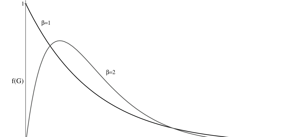
FIG. 4.: Point Contact Distribution Function.

FIG. 5.: Lowest order in $\zeta_{0}$ correction to the variance.

- [1] V.N. Prigodin, K.B. Efetov, and S. Iida, Phys. Rev. Lett. 71, 1230 (1993).
- [2] R.A. Jalabert, J.-L. Pichard, and C.W.J. Beenakker, Europhys. Lett. 27, 255 (1994).
- [3] M.L. Mehta, Random Matrices (Academic, New York, 1991).
- [4] K.B. Efetov, Adv. Phys. 32, 53 (1983).
- [5] B.L. Altshuler, V.E. Kravtsov, and I.V. Lerner, Mesoscopic Phenomena in Solids, edited by B.L. Altshuler, P.A. Lee, and R.A. Webb, (Elsevier, Amsterdam, 1991).
- [6] R. Kubo, J. Phys. Soc. Jap. 12, 570 (1957).
- [7] R. Landauer, Philos. Mag. 21, 863 (1970); M. Büttiker, Phys. Rev. Lett. 57, 1761 (1986).
- [8] V.I Fal’ko, and K.B. Efetov, Phys. Rev. B 50, 11267 (1994).
- [9] R.A. Jalabert, A.D. Stone, and Y. Alhassid, Phys. Rev. Lett. 68, 3468 (1992).
- [10] A.M. Chang, H.U. Baranger, L.N. Pfeiffer, K.W. West, and T.Y. Chang, Phys. Rev. Lett. 76, 1695 (1996); J.A. Folk, S.R. Patel, S.F. Godijn, A.G. Huibers, S.M. Cronenwett, C.M. Marcus, K. Campman, and A.C. Gossard, Phys. Rev. Lett. 76, 1699 (1996).
- [11] D.S. Fisher, and P.A. Lee, Phys. Rev. B 23, 6851 (1981).
- [12] S. Feng, C. Kane, P.A. Lee, and A.D. Stone, Phys. Rev. Lett. 61, 834 (1988).
- [13] A.A. Abrikosov, L.P. Gor’kov, and I.Y. Dzyaloshinskii, Quantum Field Theoretical Methods in Statistical Physics (Permagon, Oxford, 1965).
- [14] L.P. Gor’kov, A.I. Larkin, and D.E. Khmel’nitskii, JETP Lett. 30, 229 (1979); S. Hikami, Phys. Rev. B 24, 2671 (1981).
- [15] B. Shapiro, Phys. Rev. Lett. 57, 2168 (1986).
- [16] B. L. Altshuler, JETP Lett. 41, 648 (1985).
- [17] P. A. Lee and A. D. Stone, Phys. Rev. Lett. 55, 1622 (1985).
- [18] F.Wegner, Z. Phys. B 35 207 (1979); K.B. Efetov, A.I. Larkin, and D.E. Kheml’nitskii, Sov. Phys. JETP 52, 568 (1980).
- [19] I.V. Lerner, Phys. Lett. A 133, 253 (1988).
- [20] B.A. Muzykantskii, and D.E. Khmelnitskii, Phys. Rev. B 51, 5480 (1995). K.B. Efetov, and V.I Fal’ko, Phys. Rev. B 52, 17413 (1995).