Polaron and bipolaron formation in a cubic perovskite lattice

Abstract

The Rice-Sneddon model for BaBiO₃ is a nice model Hamiltonian for considering the properties of polarons and bipolarons in a three-dimensional oxide crystal. We use exact diagonalization methods on finite samples to study the stability and properties of polarons and bipolarons. Because polarons, when they form, turn out to be very well-localized, we are able to converge accurately our calculations for two-electron bipolaron wavefunctions, accounting for the Coulomb interaction without approximation. Some of our results are compared with and interpreted by reference to the variational method of Landau and Pekar. We calculate both electronic and vibrational excitations of the small polaron solutions, finding a single vibrational state localized with the full symmetry of the polaron, which has its energy significantly increased. Both on-site (Hubbard) and long-range Coulomb repulsion are included in the bipolaron calculation, but due to the high degree of localization, the long-range part has only a small influence. For a reasonable on-site repulsion $U$ equal to 2 times the band width $W$, bipolaron formation is significantly suppressed; there is a large window of electron-phonon coupling where the polaron is stable but the bipolaron decays into two polarons.

]

I introduction

The electron localized on an ion (or a few ions) can cause displacements of neighboring ions from their positions in the crystal lattice. The quasiparticle formed by an electron and corresponding lattice displacements is called a polaron [1]. The polaron is a small polaron if the electron is localized on a few ions or a large polaron otherwise [2]. It is possible that the surrounding ions “overscreen” the negative charge of the localized electron and attract another electron to the same site. Two electrons bound in such way form a bipolaron [2, 3]. The important issue for bipolaron formation is a quantitative analysis of the relative strength of the electron-lattice interaction responsible for two electrons being coupled and the electron-electron (Coulomb) forces which try to break the bipolaron apart. If the Coulomb repulsion between electrons exceeds some critical value the bipolaron is less stable than two separated polarons.

In present paper we study the polaron and bipolaron formation in a model originally proposed by Rice and Sneddon [4] for doped $\rm BaBiO_{3}$, such as $\rm Ba_{1-x}K_{x}BiO_{3}$ (BKBO). These materials are nearly cubic perovskites, with a fairly simple set of valence electron states, exhibiting superconducting transition temperatures as high as 30K at optimal doping. We choose this model both because of its relation to physically important materials (SrTiO₃ and WO₃ could be studied by a closely related model with $T_{2g}$ $d$-states instead of $s$-electron states) and also because it makes a nice test model for looking at the criteria for polaron formation and the properties of polarons. In this study, for simplicity, we consider the hypothetical case of an almost empty band, corresponding to KBiO₃, or BKBO with x=1.

Our principal results are (1) there is a sudden jump at a critical coupling strength from a large (delocalized) polaron to a very small, well-localized polaron; (2) the bipolaron breaks apart even at moderate strength of on-site Coulomb repulsion; and (3) small polaron formation is accompanied by a characteristic formation of localized vibrations of shifted energy which may serve as a good experimental signature.

II model Hamiltonian

The Rice-Sneddon Hamiltonian is

$$H=H_{t}+H_{e-ph}+H_{ph}+H_{C}\>,$$ (1)

where $H_{t}$, $H_{e-ph}$, $H_{ph}$ and $H_{C}$ are , correspondingly, hopping, electron-phonon, phonon, and Coulomb terms. For the hopping term, only one bismuth $s$-orbital per cell is used, with hopping only to nearest bismuth neighbors,

$$H_{t}=-t\sum_{\langle i,j\rangle\sigma}\hat{c}^{\dagger}_{i\sigma}\hat{c}_{j\sigma}\>.$$ (2)

This has the usual cosine dispersion relation with bandwidth, $W$, equal to $12t$. We take the value of $t$ to be 200 $meV$ following band-structure calculations [5]. We assume that the same model for electrons in BKBO can be applied to all the region of K concentration, because the antibonding Bi(6s)-O(2p) conduction band in cubic BKBO is minimally affected by substitutional K doping at the Ba sites[5]. First-principles LMTO calculations for different phases of BKBO: $\rm KBiO_{3}$, $\rm K_{0.5}Ba_{0.5}BiO_{3}$ and $\rm BaBiO_{3}$ reveal a single band near Fermi energy to be largely independent on potassium doping[6].

Hypothetical KBiO₃ in this model has no electrons. Each Bi atom is in the 5+ ionization state with no remaining valence electrons, whereas BaBiO₃ in this model has a half filled band of Bi⁴⁺ ions. Real BaBiO₃ is insulating, and is most simply understood as having alternating Bi³⁺ and Bi⁵⁺ ions. The Bi³⁺ ions have two valence electrons bound to them, and repel the surrounding 6 oxygen atoms, which are attracted to the more positive Bi⁵⁺ ions. A nice term for this state is that it is a “bipolaronic crystal.” The Rice-Sneddon Hamiltonian incorporates this possibility through the terms

$$H_{e-ph}=\frac{g}{a}\sum_{i\sigma}\sum_{\alpha=1}^{3}\Big{[}u_{i-,\alpha}-u_{i+,\alpha}\Big{]}\hat{c}^{\dagger}_{i\sigma}\hat{c}_{i\sigma}\>,$$ (3)

$$H_{ph}=\sum_{i}\sum_{\alpha=1}^{3}\Big{[}\frac{P^{2}_{i,\alpha}}{2M}+\frac{1}{2}M\omega_{0}^{2}u_{i,\alpha}^{2}\Big{]}\>.$$ (4)

The notation $u_{i,\alpha}$ refers to the displacement of the oxygen atom (labeled by { $i,\alpha$ } ) which neighbors the $i$-th Bi atom in the $\alpha$=x, y, z Cartesian direction. Only displacements in the direction $\hat{\alpha}$ of the bond are considered, because these are expected to dominate the physics of polaron formation. The notation $u_{i+,\alpha}$ means exactly the same as $u_{i,\alpha}$, whereas $u_{i-,\alpha}$ refers to the displacement of the oxygen atom which neighbors the $i$-th Bi atom in the $\alpha=\rm-x,-y,-z$ Cartesian direction. The atoms labeled by $(i-,\alpha)$ can also be labeled in the form $(i^{\prime},\alpha)$ by reference to the appropriate nearby Bi atom $i^{\prime}$. Eq. (3) contains the effect that an “inhaling” of the negative oxygen ions around a central Bi ion will raise the on-site energy of the bismuth $s$-orbital, by amount equal to $g$ per fractional displacement $u/a$ of each of the 6 surrounding atoms. However, this costs elastic energy as given in Eq. (4). We take M as the oxygen atomic mass, and $\omega_{0}$ to have the value 65 meV of a typical oxygen bond-stretching vibration. (It corresponds to spring energy $M\omega_{0}^{2}a^{2}/2$ being $\approx$ 4 eV.) Various values of $g$ will be used, in the physically expected range of 1-3 eV. The Bi-Bi interatomic distance $a=4.28\AA$ will be used as the unit of length, and the hopping parameter $t$ is used as the unit of energy. Finally, there is a Coulomb interaction between electrons,

$$H_{C}=U\sum_{i}\hat{n}_{i\uparrow}\hat{n}_{i\downarrow}+\sum_{i,j}\frac{e^{2}}{\varepsilon|r_{i}-r_{j}|}.$$ (5)

Various values of $U$ comparable with $W=12t$ will be used for the on-site (Hubbard) term in the Coulomb interaction, and the value $\varepsilon=5$ will characterize the long range Coulomb repulsion.

The vacuum of this model corresponds to KBiO₃, with no electrons, and only zero-point vibrational energy $3N\hbar\omega_{0}/2$. We will see that shifts of the zero point energy are not very important, so we can ignore this term and define the vacuum as having energy zero. For the half-filled case, the ground state (for not too strong Coulomb repulsion compared to electron-phonon coupling) has a period-doubling distortion of the oxygens. Alternate bismuth sites have the oxygens “breathing” either in or out, and electron charge either diminished or increased from the average of one electron per site. This corresponds to the experimental insulating state of BaBiO₃, and gives a new vacuum into which carriers can be introduced by doping. Neglecting Coulomb repulsion, this regime was was studied numerically by Yu et al. [7], who found, in agreement with experiment, that the insulating gap persisted for a wide range of K-doping. In d=2, this model was studied by Prelovšek et al. using an adiabatic treatment of the phonon degrees of freedom and the Hartree approximation for the Hubbard term [8].

III polaron

Our only approximation (apart from finite size errors which are well-controlled) is the Born-Oppenheimer (adiabatic) treatment of the vibrations. Inserting one electron into the empty-band vacuum, and letting the oxygen atoms have some fixed distortion pattern $\{u\}$, we look for the lowest energy one-electron state with wavefunction

$$\psi_{\uparrow}(\{u\})=\sum_{i}a_{i}(\{u\})c^{\dagger}_{i,\uparrow}|\rm{vac}\rangle\>,$$ (6)

where $a_{i}(\{u\})$ are the site amplitudes of the electron wave function. Later the dependence of $a_{i}$ etc. on the parameters $\{u\}$ will be implicit and not explicitly designated. This electron state has energy $\epsilon_{0}(\{u\})$, measured relative to the bottom of the band, $\epsilon_{0}(\{0\})$. The total energy is this plus the elastic energy $\langle H_{ph}(\{u\})\rangle$. Then we vary the displacements $\{u\}$ looking for the absolute minimum total energy. If the coupling constant $g$ is small, the minimum occurs at $\{u\}=\{0\}$ and has total energy 0. This corresponds to a large polaron solution, which in adiabatic approximation is just an electron in the bottom of the band of the undeformed crystal. If we were to include the non-adiabatic coupling of this electron with virtual phonons, there would be an alteration of the mass and energy of this electron. Specifically, the energy shift would be

$$\Delta\epsilon_{0}=\sum_{j,k}\frac{|M_{0j}^{k}|^{2}}{\epsilon_{0}-\epsilon_{j}-\hbar\omega_{k}}\\$$ (7)

in terms of the one electron energies $\epsilon_{j}$ and the phonon energies $\hbar\omega_{k}$ of the unperturbed band. This sum can be evaluated as follows,

$$\frac{\Delta\epsilon_{0}}{t} = \left(\frac{g}{t}\right)^{2}\frac{\hbar\omega_{0}}{2M\omega_{0}^{2}a^{2}}\left[1-S\left(\frac{\hbar\omega_{0}}{4t}\right)\right],$$ (8)

$$S(x) = \frac{1}{N}\sum_{\vec{Q}}\frac{x}{x+f({\bf Q})}\>,$$ (9)

$$f({\bf Q}) = sin^{2}(\frac{Q_{x}a}{2})+sin^{2}(\frac{Q_{y}a}{2})+sin^{2}(\frac{Q_{z}a}{2})\>.$$ (10)

For our choices of $\omega_{0}$ and $t$, the ratio $\hbar\omega_{0}/4t$ is 0.081 and the sum $S$ in Eq. (9) is 0.05. Thus the self-energy shift of the large polaron is $\approx 4\times 10^{-3}\times(g/t)^{2}$ which turns out to be small compared to the energies that we will find for the small polaron regime. Thus we can safely ignore the non-adiabatic effects. By a similar argument (which we will explain in more detail later) the zero-point contribution to the elastic energy can be ignored, and our elastic contribution to the small polaron energy is just the second term of Eq. (4).

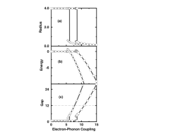
FIG. 1.: Calculated properties of a polaron: (a) radius $r_{P}/a$, (b) total energy per electron $E_{\rm tot}/t$, and (c) the gap $(\epsilon_{1}-\epsilon_{2})/t$ in the electron spectrum as a function of electron-phonon coupling $g/t$. The circles give results for the single-electron polaron and the diamonds give the radius, half the total energy, and the electronic gap for the bipolaron. The Coulomb repulsion is omitted for the bipolaron ($U=U^{\prime}=0$).

To evaluate the one-electron energy $\epsilon_{0}(\{u\})$ for the distorted lattice requires a finite size system, which we choose to be an orthorhombic cell (our “supercell”) with $N=N_{1}\times N_{2}\times N_{3}$ Bi atoms on a cubic lattice, and 3$N$ oxygens on the Bi-Bi bonds, and periodic boundary conditions. The Lanczos technique [9] was used for finding the ground state energy and a few lowest excited states of the Hamiltonian (1), and conjugate gradient minimization was used to find the optimum values of the oxygen displacements $\{u\}$. Beyond a critical value $(g/t)_{c}$=8.57 it becomes favorable for oxygens to distort and form a localized small polaron state. We define the location $\vec{r}_{0}$ and radius $r_{P}$ of the polaron by

$$\vec{r}_{0}=\sum_{i}|a_{i}|^{2}\vec{r}_{i}\>,$$ (11)

$$r_{P}^{2}=\sum_{i}|a_{i}|^{2}(\vec{r}_{i}-\vec{r}_{0})^{2}\>.$$ (12)

The radius of the polaron at the transition is 0.49 in units of Bi-Bi distance, that is, it is very well-localized with 90% of the electron density concentrated on one site. As $g$ increases beyond the critical value, the radius further shrinks, and the binding energy rapidly increases to values of order $t$ and bigger.

Our results are plotted in Fig. 1. For $g/t$ less than the critical value, the radius is shown as a finite number, $\approx 4a$, reflecting the finite size of the cell; the actual radius is infinite. For values of $g/t$ slightly less than critical, our minimization proceedure locates a metastable small polaron solution with a small positive energy, which is shown in Fig. 1 as a small hysteretic region.

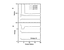
FIG. 2.: Tests of finite-size errors for different values of electron-phonon coupling constants. The cluster radius is in the units of the Bi-Bi distance. The clusters used are $N_{0}\times N_{0}\times N_{0}$ and $(N_{0}-1)\times N_{0}\times(N_{0}+1)$, out to a maximum of $N_{0}$ of 20. The cluster radius is $N_{0}$ in the former case or $N_{0}^{1/3}(N_{0}^{2}-1)^{1/3}$ in last case.

Because the small polaron is so well-localized, the error in our calculation due to the finite size supercell is easy to control. To test this, we have varied the size of the supercell from a minimum of $2\times 2\times 2$ to maximum of $20\times 21\times 22$. The results are shown in Fig. 2. The polaron radius and total energy are insensitive to cluster size if the number of Bi-atoms is $\gtrsim 200$. Near the transition, for cluster size not too big, the transition onset varies with cluster size. The total energy always diminishes with increase of cluster size until it becomes independent of cluster size. At $g/t$ far enough from the critical value the results are almost the same for all the clusters sizes. The results of Fig. 1 have no noticeable size dependence.

The non-adiabatic corrections to the large polaron energy are 0.0064$t$ at the transition point, which gives an unimportant correction to the critical value of $g/t$. The small polaron solution is $2N$-fold degenerate: it can form at any of the $N$ Bi sites, with either spin. In this paper we ignore another non-adiabatic effect, the weak vibration-assisted tunnelling which lifts the translational degeneracy to make a narrow band with only spin degeneracy remaining.

FIG. 3.: Total energy versus polaron radius calculated in Landau-Pekar approximation for electron-phonon coupling constants $g/t$=0., 8.23, 10., 12., and 15. from top to bottom. The energy minima for $g/t$= 10., 12., and 15. correspond to energies of stable localized states. The extremum at $g/t$=8.23 corresponds to a metastable localized state. Results from finite cluster diagonalization are shown as X’s. For numerical comparison see Table 1. The inset expands the large $r_{P}$ part of the same curves.

We now compare our numerical results with analytic results obtained by a variational method introduced by Landau and Pekar (LP) [10, 11]. The electronic wave function is chosen to have Gaussian form

$$a_{i}=C_{0}(\beta)\exp(-\beta^{2}(\vec{r}_{i}-\vec{r}_{0})^{2}/2)\>,$$ (13)

where $C_{0}$ is the normalization constant and $\beta$ is the variational parameter which we call the LP parameter. There are now two sequential minimizations to perform [12]. First for fixed $\beta$ the optimum displacements $\{u(\beta)\}$ are found. Then these are used to evaluate the trial total energy $E(\beta)$, and a second minimization is performed to find the optimum $\beta$. We find analytic formulas for $E(\beta)$ and the polaron radius $r_{P}(\beta)$,

$$E(\beta) = -6tq^{1/4}\frac{\theta_{2}(q)}{\theta_{3}(q)}-3\frac{{\rm g}^{2}}{M\omega_{0}^{2}}\frac{\theta_{3}(q^{2})^{2}}{\theta_{3}(q)^{6}}$$ (14)

$$\times [\theta_{3}(q^{2})-q^{1/2}\theta_{2}(q^{2})]\>,$$ (15)

$$r_{P}(\beta)^{2} = 6q\theta_{3}^{\prime}(q)/\theta_{3}(q)\>,$$ (16)

where $q={\rm exp}(-\beta^{2})$ and $\theta_{i}(q)=\theta_{i}(0,q)$ are Jacobi’s theta functions [13]. $\theta_{3}^{\prime}(q)$ is the derivative of $\theta_{3}(q)$. These equations define an implicit function $E(r_{P})$ which is plotted in Fig. 3 for the values $g/t$ equal to 0., 8.229, 10., 12. and 15. X-marks indicate the exact results from our finite cluster calculations. The agreement is remarkable, especially, for the values of minimal total energy (see Table 1). The LP solution gives a smaller value of the polaron radius. The variational solution for an infinite system agrees with the exact solution on finite clusters in finding a first-order large to small polaron transition, with no intermediate regime of large polarons exist. Figure 3 explains the hysteresis found in the numerical results obtained by exact-diagonalization. For a small range of $g$ just below the critical value the small polaron state is locally stable but separated by an energy barrier from the global (delocalized) minimum. The numerical solution follows this metastable branch until it disappears.

TABLE I.: Comparison of results obtained by Landau-Pekar (LP) variational method and by exact diagonalization of finite clusters (cluster). The electron-phonon coupling constants are in units of bandwidth ($W=12t$). The first row in the table corresponds to the critical coupling constant at which a metastable localized state occurs. The total energies $E_{\rm total}^{\rm LP}$ and $E_{\rm total}^{\rm cluster}$ are in units of $t$. The polaron radius is given in units of the Bi-Bi distance. Cluster calculations give a slightly smaller total energy and larger radius. The phonon spectrum is perturbed by the transition from delocalized state to localized (see text). In LP approximation only one mode, $\omega_{\rm max}^{\rm LP}$ changes from its initial value of $\omega_{0}$. In the cluster calculations, one mode, $\omega_{\rm max}^{\rm cluster}$, is well-separated from the others.

$g/W$	$E_{\rm total}^{\rm LP}$	$E_{\rm total}^{\rm cluster}$	$r_{p}^{\rm LP}$	$r_{p}^{\rm cluster}$	$\omega_{\rm max}^{\rm LP}/\omega_{0}$	$\omega_{\rm max}^{\rm cluster}/\omega_{0}$
0.686	0.398	0.377	0.448	0.490	1.176	1.163
0.833	-1.848	-1.853	0.290	0.299	1.075	1.065
1.000	-5.040	-5.041	0.198	0.200	1.035	1.028
1.250	-11.03	-11.03	0.126	0.126	1.014	1.011

IV Electronic and vibrational excitations of the polaron

An advantage of the exact diagonalization method is that is enables an equally good and easy calculation of electronic excitations of the Franck-Condon type where the lattice distortion is frozen in place. We simply examine the next higher-lying eigenstates without further alteration of the parameters $\{u\}$. In the range of parameter space we have explored, we have not encountered a second bound state in the polaronic well. The electronic spectrum has a gap, and the minimum energy electronic excitation is a delocalized state. The energy of this transition, denoted the “gap” energy, is plotted in Fig. 1.c. At the onset of polaron formation, the gap has a value $5.00t$ which increases rapidly for larger coupling constants. There is a small but noticeable finite size error in the gap calculation since the lowest electronic excited state is extended to infinity, but cut off at the supercell boundary in our work.

When a small polaron is formed, the interaction between the localized electron and the lattice vibrations can cause both a renormalization of the electron energy and of the phonon energy. Referring to Eq. (7), it is clear that the gap, or minimum value of $\epsilon_{0}-\epsilon_{j}$ in the denominator, makes a change in the electron self-energy shift relative to the one already calculated for the delocalized large polaron, probably reducing the shift because of the larger denominator (although matrix element changes need to be considered also.) However, since the shift is certainly small compared to the gap itself (of order $t$), this effect can be neglected.

A more interesting effect is the change in the local vibrations near the localized electron. If we know the one-electron energies $\epsilon_{j}$ and the corresponding states $|j\rangle$ at the optimal set of displacements $\{u_{0}\}$, then standard perturbation theory for small displacements around these displacements gives

$$\Delta\left[\frac{\partial^{2}E_{{\rm tot}}}{\partial u_{\ell,\alpha}\partial u_{\ell^{\prime},\beta}}\right] = \sum_{j}\frac{\langle 0|V_{\ell,\alpha}|j\rangle\langle j|V_{\ell^{\prime},\beta}|0\rangle}{\epsilon_{0}-\epsilon_{j}}\>,$$ (17)

$$V_{\ell,\alpha} = \frac{\partial H_{e-ph}}{\partial u_{\ell,\alpha}}\>.$$ (18)

This equation omits terms containing second derivatives of $H$ because they are consistently omitted in our model.

The LP approximation gives a particularly simple solution to this problem. Since we don’t have a complete set of states in this approach, instead, we find the energy as a general function of the displacements $\{u_{0}\}$ and the LP parameter $\beta$,

$$E(\vec{u},\beta)=\frac{1}{2}\vec{u}^{\dagger}\cdot\hat{A}\cdot\vec{u}+\vec{L}^{\dagger}(\beta)\cdot\vec{u}+f(\beta)\>,$$ (19)

where $\vec{u}$ is the $3N$-vector displacement, $\hat{A}$ is the bare force constant matrix (which is a constant times the unit matrix in our model), $\vec{L}$ is the force on the atoms caused by the localized electron, and $f$ is the localized electron hopping energy. Expressions for $\vec{L}$ and $f$ are easy to derive. Straightforward linear algebra leads to expressions for the optimum values $\{u_{0}\}$ and $\beta_{0}$. We then Taylor-expand Eq. (19) to second order for small deviations $\{\delta u\}$ and $\delta\beta$ around the optimum values. Finally, for fixed deviations $\{\delta u\}$ the optimum value of $\delta\beta$ is found. Inserting this into the Taylor expansion, the modified force constant matrix $\hat{A}^{\prime}$ is found,

$$\hat{A}^{\prime}=\hat{A}+\frac{\vec{L^{\prime}}\vec{L^{\prime}}^{\dagger}}{\vec{L}^{\dagger}\cdot\hat{A}^{-1}\cdot\vec{L^{\prime\prime}}-f^{\prime\prime}}\>.$$ (20)

The primes on the right hand side of Eq. (20) denote derivatives by $\beta$. Note that the alteration of the force constant matrix in LP approximation is factorizable, and since $\hat{A}$ is proportional to the unit matrix, only one eigenvalue is altered, the corresponding eigenvector being proportional to $\vec{L^{\prime}}$. The static displacements $\{u_{0}\}$ in LP approximation are given by $-\hat{A}^{-1}\vec{L}(\beta_{0})$. Thus in LP approximation, one vibrational eigenvector splits off from the degenerate frequency $\omega_{0}$, shifting to higher energy, and having an eigenvector proportional to the derivative of the static displacements by the LP parameter $\beta$. The symmetry of this mode is identical to the symmetry of the static displacement.

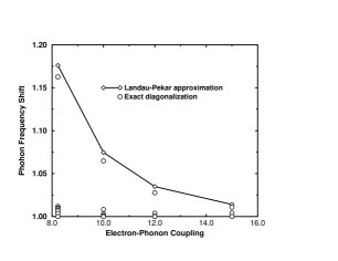
FIG. 4.: Phonon frequency shifts, $\omega_{ph}^{i}/\omega_{0}$, at coupling constants $g/t$=8.23, 10., 12., and 15. for cluster size $5\times 6\times 7$. The phonon modes (circles) are distributed from $\omega_{0}$ to $\omega_{\rm max}$, the last being well separated from others. Results from the Landau-Pekar approximation are shown by diamonds.

We have also made an exact calculation of the modified vibrational spectrum using finite clusters, and the answers, shown in Fig. 4, and also in Table 1, agree nicely with the LP approximation, but in addition to the one strongly altered frequency, a few other frequencies are pulled weakly above the unperturbed frequency $\omega_{0}$.

Thus we expect that a characteristic signature of the small polaron state should be a localized vibrational mode whose symmetry copies that of the polaronic distortion, that is, the symmetry is the same as the point symmetry in the crystal of the ion on which the polaron is centered (full cubic symmetry $A_{1}$ in our case.) Such modes might be measureable by Raman scattering using a laser which is resonant with an electronic transition of the polaron. Also they might appear as side-bands on the electronic polaron absorption spectrum.

V bipolaron

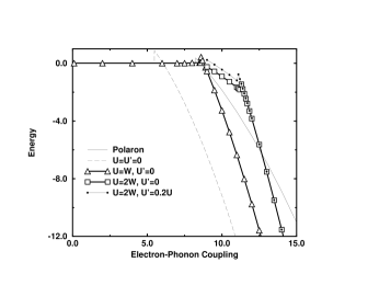
FIG. 5.: Total energy (per electron) of the bipolaron for different values of Coulomb repulsion. The supercell size is $5\times 6\times 7$. At $U=2W$ for $g/t$ between 8.6 and 11.3, the total energy corresponds to two small polarons separated as far as possible in the cell; because the cell is not infinitely large, there is Coulomb repulsion which raises the energy above the isolated polaron energy shown as the thin curve (identical to Fig. 1).

We now ask what happens in our model when a second electron is added. If we neglect the Coulomb interaction, the answer is that two spatially separated polarons are unstable relative to formation of a singlet bipolaron state in which both electrons are on the same site. If we allow no further lattice relaxation beyond the single electron polaron, then the energy of the bipolaron is already lower than two separated polarons because the (negative) electronic eigenvalue is doubled but the positive lattice strain energy is unchanged; additional lattice relaxation will occur only if it lowers the energy, and since there are now two electrons exerting each force $g$ on the neighboring oxygens, there will be additional relaxation. Results are shown in Fig. 1 where we plot the total energy per electron. The critical coupling for bipolaron formation is $g/t$=6.08, significantly less than for polaron formation which starts at $g/t$=8.57. At onset of bipolaron formation, the radius and the electronic gap (0.44$a$ and 5.00$t$, respectively) are approximately the same as for polaron formation at its onset, but at equal values of $g$ the bipolaron is smaller and has a larger gap.

Of course it is unrealistic to ignore the Coulomb repulsion which will act in the direction of destabilizing the bipolaron. Our model permits us to make exact (finite size) calculations for the bipolaron by solving the appropriate two-particle equation, that is, finding the exact two-particle wavefunction

$$\Psi(\{u\})=\sum_{i,j}a_{i,j}(\{u\})c^{\dagger}_{i,\uparrow}c^{\dagger}_{j,\downarrow}|\rm{vac}\rangle.$$ (21)

This calculation is of course far more demanding than the corresponding polaron case, Eq. (6), because it requires on each step of the minimization procedure finding the smallest eigenvalues of a $N^{2}\times N^{2}$ matrix rather than a $N\times N$ matrix. Our Lanzcos algorithm has allowed us to calculate for $N$ as large as $5\times 6\times 7$. Because the bipolaron turns out to be again well- localized, the finite system size does not cause a noticeable error. Also for the same reason, the long-range Coulomb repulsion is not very important.

FIG. 6.: Bipolaron radius as a function of $g/t$ for different values of Coulomb repulsion. Vertical lines indicate stability limits where bipolarons (with $U{\lesssim}W$) decay into isolated small polarons, or into isolated large polarons when $U{\gtrsim}W$. At $g/t$ less than the stability point, radii of metastable bipolaron states are shown. The domain of metastability is artificially enhanced by finite size effects.

Results for the bipolaron radius, energy, and excitation gap are shown in Figs. 5, 6, and 7. The onsite Coulomb strength $U$ (see Eq. (5)) is estimated as $e^{2}/2r_{\rm Bi}$, while the long-range Coulomb interaction is characterized by a parameter we call $U^{\prime}=e^{2}/\varepsilon a$. For $r_{\rm Bi}=0.5$ and $\varepsilon=5$ one finds $U$ = 3.5 eV = 1.46$W$ and $U^{\prime}$ = 0.7 eV = 0.29$W$, where the bandwidth $W$ is $12t$ or $\approx 2.4$ eV. Our calculations are shown for the cases $U/W$= 1 and 2 with $U^{\prime}$=0, and for $U/W$= 2 with $U^{\prime}$= 0.2. Fig. 5 shows that on-site Coulomb repulsion with the small value of $U=W$ destabilizes the bipolaron until $g/t$ reaches 8.95, slightly beyond the stability point $g/t=8.57$ for the polaron. A more physical choice of $U=2W$ prevents stable bipolaron formation until $g/t\approx$ 12.8. Our numerical solutions show bipolarons winning over separated polarons at somewhat smaller values of coupling constants ($g/t=8.60$ for $U=W$ and $g/t=11.3$ for $U=2W$.) This is a finite size error caused by the fact that in our cell, two separated polarons are only separated by half the cell diagonal, and have a small repulsion which artificially raises their energy, favoring bipolarons for smaller coupling than would be the case in a very large cell. But since we have already an accurate answer for the energy of two well-separated polarons, our numerics tells us the true stability point. As is seen in Fig. 5, there is also a small hysteretic regime indicating that the transition from separated polarons to bipolarons is first order. As is seen in Fig. 5, adding the long-range Coulomb term ($U^{\prime}=0.2U$) causes a small additional postponement of bipolaron formation, but hardly alters the properties for values of $g/t$ where it is stable.

The radius shown in Fig. 6 is defined exactly as in Eq. (12) after defining the probability $|a_{i}^{\prime}|^{2}$ for finding an electron on site $i$ in the usual way,

$$|a_{i}^{\prime}|^{2}=\sum_{j}|a_{i,j}|^{2}\>.$$ (22)

Fig. 6 shows that the radius of the bipolaron is increased by increasing the value of $U$, but decreased by increasing the value of $U^{\prime}$. In all cases the bipolaron has a smaller radius than the polaron at the same value of $g$.

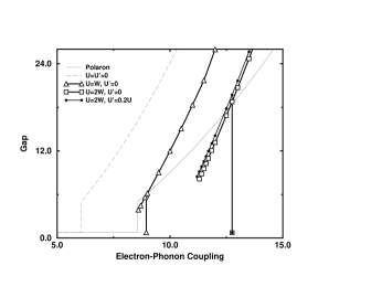
FIG. 7.: The gap in the electron spectrum as a function of $g/t$. Due to finite size of cluster the gap is finite even in delocalized state.

An interesting feature shown in Fig. 7 is that the gap is larger at the onset of bipolaron formation in the presence of the long-range Coulomb repulsion, presumably due to stronger localization of electrons. At fixed $g/t$ the Coulomb forces reduce the gap with increasing $U$.

VI summary

Bipolaron formation is strongly affected by Coulomb forces in a cubic perovskite lattice. Due to Coulomb repulsion between two electrons localized on the same site the onset of bipolaron formation can be postponed and polaron states are energetically favorable. The polarons and bipolarons formed in this lattice are small and exist only above some critical value of electron-phonon coupling. The transition from delocalized to localized polaron state is discontinuous, with no intermediate- size solution. This jump is not caused by finite-size errors and is present also in variational calculations using Landau-Pekar approximation. The total energy has hysteretic behavior with metastable states occuring near the critical coupling constant. These metastable states could in principal be observed, for example, by tuning the coupling constant with applied pressure. A gap opens in the electron spectrum at the transition from delocalized to localized polaron states, and new localized vibrational states occur with energies increased above those of the undoped host.

- [1] The concept of the polaron was first introduced by L. D. Landau in Phys. Z. Sowjetunion 3, 664 (1933).
- [2] A. S. Alexandrov and N. F. Mott, Polarons and Bipolarons (World Scientific, Singapore, 1995).
- [3] N. F. Mott, Metal-Insulator Transitions, 2nd ed. (Taylor & Francis, London, 1990).
- [4] T. M. Rice and L. Sneddon, Phys. Rev. Lett. 47, 689 (1981).
- [5] L. F. Mattheiss and D. R. Hamann, Phys. Rev. Lett. 60, 2681 (1988).
- [6] W. D. Mosley et al., Phys. Rev. Lett. 73, 1271 (1994).
- [7] J. Yu, X. Y. Chen, and W. P. Su, Phys. Rev. B 41, 344 (1990).
- [8] P. Prelovšek, T. M. Rice, and F. C. Zhang, J. Phys. C 20, L229 (1987).
- [9] J. K. Cullum and R. A. Willoughby, Lanczos Algorithms for Large Symmetric Eigenvalue Computations, v. 1-2 (Birkhäuser, Boston, 1985).
- [10] L. P. Landau and S. I. Pekar, Zh. Eksp. Teor. Fiz. 16, 341 (1946).
- [11] S. J. Miyake, J. Phys. Soc. Japan 41, 747 (1976).
- [12] G. D. Mahan, Many-Particle Physics (Plenum Press, New York, 1990).
- [13] Handbook of Mathematical Functions, edited by M. Abramowitz and I. A. Stegun (Dover Publications, New York, 1972).