Phase-dependent magnetoconductance fluctuations in a chaotic Josephson junction

The conductance of a mesoscopic metal shows small fluctuations of universal size $e^{2}/h$ as a function of magnetic field.[1] These universal conductance fluctuations are sample-specific, which is why a plot of conductance $G$ versus magnetic field $B$ is called a “magnetofingerprint”. The magnetoconductance is sample-specific because it depends sensitively on scattering phase shifts, and hence on the precise configuration of scatterers. Any agency which modifies phase shifts will modify the magnetoconductance. Altshuler and Spivak[2] first proposed to use a Josephson junction for this purpose. If the metal is connected to two superconductors with a phase difference $\phi$ of the order parameter, the conductance $G(B,\phi)$ contains two types of sample-specific fluctuations: aperiodic fluctuations as a function of $B$ and $2\pi$-periodic fluctuations as a function of $\phi$. The magnetic field should be sufficiently large to break time-reversal symmetry, otherwise the sample-specific fluctuations will be obscured by a much stronger $B$- and $\phi$-dependence of the ensemble-averaged conductance.[3, 4]

In a recent Letter, Den Hartog et al.[5] reported the experimental observation of phase-dependent magnetoconductance fluctuations in a T-shaped two-dimensional electron gas. The horizontal arm of the T is connected to two superconductors, the vertical arm to a normal metal reservoir. The observed magnitude of the fluctuations was much smaller than $e^{2}/h$, presumably because the motion in the T-junction was nearly ballistic. Larger fluctuations are expected if the arms of the T are closed, leaving only a small opening (a point contact) for electrons to enter or leave the junction. Motion in the junction can be ballistic or diffusive, as long as it is chaotic the statistics of the conductance fluctuations will only depend on the number of modes in the point contacts and not on the microscopic details of the junction.

In this paper we present a theory for phase-dependent magnetoconductance fluctuations in a chaotic Josephson junction. We distinguish two regimes, depending on the relative magnitude of the number of modes $M$ and $N$ in the point contacts to the superconductors and normal metals respectively. For $M\gg N$ the $\phi$-dependence of the conductance is strongly anharmonic. This is the regime studied by Altshuler and Spivak.[2] For $M\lesssim N$ the oscillations are nearly sinusoidal, as observed by Den Hartog et al.[5] The difference between the two regimes can be understood qualitatively in terms of interfering Feynman paths. In the regime $M\lesssim N$ only paths with a single Andreev reflection contribute to the conductance. Each such path depends on $\phi$ with a phase factor $e^{\pm i\phi/2}$. Interference of these paths yields a sinusoidal $\phi$-dependence of the conductance. In the opposite regime $M\gg N$, quasiparticles undergo many Andreev reflections before leaving the junction. Hence higher harmonics appear, and the conductance becomes a random $2\pi$-periodic function of $\phi$.

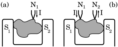
FIG. 1.: Josephson junction in a three-terminal (a) and four-terminal (b) configuration.

The system under consideration is shown schematically in Fig. 1. It consists of a chaotic cavity in a time-reversal-symmetry breaking magnetic field $B$, which is coupled to two superconductors and to one or two normal metals by ballistic point contacts. The superconductors (S₁ and S₂) have the same voltage (defined as zero) and a phase difference $\phi$. The conductance of this Josephson junction is measured in a three- or four-terminal configuration. In the three-terminal configuration (Fig. 1a), a current $I$ flows from a normal metal N₁ into the superconductors. The conductance $G=I/V_{1}$ is the ratio of $I$ and the voltage difference $V_{1}$ between N₁ and S₁, S₂. This corresponds to the experiment of Den Hartog et al.[5] In the four-terminal configuration (Fig. 1b), a current $I$ flows from a normal metal N₁ into another metal N₂. The conductance $G=I/(V_{1}-V_{2})$ now contains the voltage difference between N₁ and N₂. This is the configuration studied by Altshuler and Spivak.[2]

Following Ref. [5] we split the conductance $G(B,\phi)=G_{0}(B)+G_{\phi}(B,\phi)$ into a $\phi$-independent background

$$G_{0}(B) = \int_{0}^{2\pi}{d\phi\over 2\pi}\,G(B,\phi),$$ (1)

plus $2\pi$-periodic fluctuations $G_{\phi}$. In the absence of time-reversal symmetry, the ensemble average $\langle G(B,\phi)\rangle\equiv\langle G\rangle$ is independent of $B$ and $\phi$. Hence $\langle G_{0}(B)\rangle=\langle G\rangle$ and $\langle G_{\phi}(B,\phi)\rangle=0$. The correlator of $G$ is

$$C(\delta B,\delta\phi) = \langle G(B,\phi)G(B+\delta B,\phi+\delta\phi)\rangle-\langle G\rangle^{2}.$$ (2)

Fluctuations of the background conductance are described by the correlator of $G_{0}$,

$$C_{0}(\delta B) = \langle G_{0}(B)G_{0}(B+\delta B)\rangle-\langle G\rangle^{2}$$ (3)

$$= \int_{0}^{2\pi}{d\delta\phi\over 2\pi}\,C(\delta B,\delta\phi).$$ (4)

(In the second equality we used that $\langle G_{\phi}G_{0}\rangle=0$.) The difference $C_{\phi}=C-C_{0}$ is the correlator of $G_{\phi}$,

$$C_{\phi}(\delta B,\delta\phi) = \langle G_{\phi}(B,\phi)G_{\phi}(B+\delta B,\phi+\delta\phi)\rangle.$$ (5)

We compute these correlators for the three- and four-terminal configurations, beginning with the former.

In the three-terminal configuration, the cavity is connected to three point contacts (Fig. 1a). The contact to the normal metal has $N$ propagating modes at the Fermi energy, the contacts to the superconductors have $M/2$ modes each. The $(N+M)\times(N+M)$ scattering matrix $S$ of the cavity is decomposed into $M\times M$ ($N\times N$) reflection matrices $r$ ($r^{\prime}$) and $N\times M$ ($M\times N$) transmission matrices $t$ ($t^{\prime}$),

$$S=\left(\begin{array}[]{cc}r&t^{\prime}\\ t&r^{\prime}\end{array}\right).$$ (6)

The conductance at zero temperature is determined by the matrix $s_{he}$ of scattering amplitudes from electron to hole,[6, 7]

$$G = 2\,\mbox{tr}\,s_{he}^{\vphantom{dagger}}s_{he}^{\dagger},$$ (8)

$$s_{he}{\vphantom{dagger}} = -i\,t^{*}\left(1+e^{i\Phi}re^{-i\Phi}r^{*}\right)^{-1}\!e^{i\Phi}t^{\prime}.$$ (9)

The diagonal matrix $\Phi$ has diagonal elements $\Phi_{nn}=\phi/2$ if $1\leq n\leq M/2$ and $-\phi/2$ if $1+M/2\leq n\leq M$. We measure $G$ in units of $2e^{2}/h$.

For chaotic scattering without time-reversal symmetry, the matrix $S$ is uniformly distributed in the unitary group.[8] This is the circular unitary ensemble (CUE) of random-matrix theory.[9] The CUE does not specify how $S$ at different values of $B$ is correlated. The technical innovation used in this work is an extension of the CUE, which includes the parametric dependence of the scattering matrix on the magnetic field. The method (described in detail elsewhere[10]) consists in replacing the magnetic field by a time-reversal-symmetry breaking stub (see Fig. 2). This idea is similar in spirit to Büttiker’s method of modeling inelastic scattering by a phase-breaking lead.[11] The stub contains $N_{\rm stub}$ modes. The end of the stub is closed, so that it conserves the number of particles without breaking phase coherence. (Büttiker’s lead, in contrast, is attached to a reservoir, which conserves the number of particles by matching currents, not amplitudes, and therefore breaks phase coherence.) We choose our scattering basis such that the $N_{\rm stub}\times N_{\rm stub}$ reflection matrix $r_{\rm stub}(B)$ of the stub equals the unit matrix at $B=0$. For non-zero magnetic fields we take

$$r_{\rm stub}(B)=e^{BA},\ \ a^{2}\equiv\sum_{n<m}A_{nm}^{2},$$ (10)

where the matrix $A$ is real and antisymmetric: $A_{nm}^{\vphantom{*}}=A_{nm}^{*}=-A_{mn}^{\vphantom{*}}$. Particle-number is conserved by the stub because $r_{\rm stub}$ is unitary, but time-reversal symmetry is broken, because $r_{\rm stub}$ is not symmetric if $B\neq 0$. In order to model a spatially homogeneous magnetic field, it is essential that $N_{\rm stub}\gg N+M$. The value of $N_{\rm stub}$ and the precise choice of $A$ are irrelevant, all results depending only on the single parameter $a$.

The magnetic-field dependent scattering matrix $S(B)$ in this model takes the form

$$S(B)=U_{11}+U_{12}\left[1-r_{\rm stub}(B)U_{22}\right]^{-1}r_{\rm stub}(B)U_{21}.$$ (11)

The matrices $U_{ij}$ are the four blocks of a matrix $U$ representing the scattering matrix of the cavity at $B=0$, with the stub replaced by a regular lead. The distribution of $U$ is the circular orthogonal ensemble (COE), which is the ensemble of uniformly distributed, unitary and symmetric matrices.[9] The distribution of $S(B)$ resulting from Eqs. (10) and (11) crosses over from the COE for $B=0$ to the CUE for $B\to\infty$. One can show[10] that it is equivalent to the distribution of scattering matrices following from the Pandey-Mehta Hamiltonian[12] $H=H_{0}+iBH_{1}$ [where $H_{0}$ ($H_{1}$) is a real symmetric (antisymmetric) Gaussian distributed matrix].

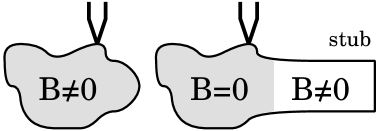
FIG. 2.: Schematic picture how the magnetic field is included in the scattering-matrix ensemble. A chaotic cavity with a spatially homogeneous magnetic field (left diagram) is statistically equivalent to a chaotic cavity in zero magnetic field (right diagram), which is coupled to a closed lead (a stub) having a non-symmetric reflection matrix.

It remains to relate the parameter $a$ to microscopic properties of the cavity. We do this by computing the correlator $\Sigma_{mn}(\delta B)=\langle S_{mn}^{\vphantom{*}}(B)S_{mn}^{*}(B+\delta B)\rangle$ from Eq. (11). Using the diagrammatic method of Ref. [13] to perform the average over the COE, we find (for $N+M\gg 1$)

$$\Sigma_{mn} = (N+M)^{-1}\left[1+(\delta B/B_{c})^{2}\right]^{-1},\ \ n\neq m,$$ (12)

with $B_{c}\equiv a^{-1}\sqrt{N+M}$. This correlator of scattering matrix elements has also been computed by other methods.[14, 15, 16, 17] Comparing results we can identify

$$a^{2}=ce^{2}v_{F}L^{2}\min(\ell,L)/\hbar\delta,$$ (13)

with $c$ a numerical coefficient of order unity depending on the shape of the cavity (linear dimension $L$, mean free path $\ell$, Fermi velocity $v_{F}$, level spacing $\delta$). For example, for a disordered disk or sphere (radius $L\gg\ell$) the coefficient $c=\pi/8$ for the disk and $\pi/15$ for the sphere.

We now proceed with the calculation of the correlator of the conductance. We consider broken time-reversal symmetry ($B\gg B_{c}$) and assume that $N$ and $M$ are both $\gg 1$. Using the method of Ref. [13] for the average over $U$, we obtain the average conductance $\langle G\rangle=2NM/(N+2M)$ and the correlator

$$C(\delta B,\delta\phi)={16KN^{2}M^{2}(N+M)^{2}}{(N+2M)^{-4}}$$ (14)

$$\mbox{}\times{(N+M)^{2}+(N^{2}+M^{2}K)\cos^{2}(\delta\phi/2)\over\left[(N+M)^{2}-M^{2}K\cos^{2}(\delta\phi/2)\right]^{2}},$$ (15)

where we have abbreviated $K=\left[1+(\delta B/B_{c})^{2}\right]^{-2}$. Eq. (14) simplifies considerably in the two limiting regimes $M\ll N$ and $M\gg N$. For $M\ll N$ we find

$$C_{0}(\delta B) = 24(M/N)^{2}K,$$ (17)

$$C_{\phi}(\delta B,\delta\phi) = 8\left({M/N}\right)^{2}K\cos\delta\phi,$$ (18)

whereas for $M\gg N$ we have (for $|\delta\phi|<\pi$)

$$C_{0}(\delta B) = {\sqrt{N\over 8M}}\left[1+{M\over N}\left({\delta B\over B_{c}}\right)^{2}\right]^{-3/2},$$ (20)

$$C_{\phi}(\delta B,\delta\phi) = {1\over 2}\left[1+{M\over N}\left({\delta B\over B_{c}}\right)^{2}+{M\over 8N}{\delta\phi}^{2}\right]^{-2}.$$ (21)

The two regimes differ markedly in several respects:

(1) The $2\pi$-periodic conductance fluctuations are harmonic if $M\ll N$ and highly anharmonic if $M\gg N$. A small increment $\delta\phi\simeq\sqrt{N/M}\ll 2\pi$ of the phase difference between the superconducting contacts is sufficient to decorrelate the conductance if $M\gg N$.

(2) The variance of the conductance $\mbox{var}\,G=C_{0}(0)+C_{\phi}(0,0)$ has the universal magnitude $1/2$ if $M\gg N$, while it is reduced by a factor $(8M/N)^{2}$ if $M\ll N$.

(3) The variance $\mbox{var}\,G_{\phi}=C_{\phi}(0,0)$ of the $\phi$-dependent conductance is larger than the variance $\mbox{var}\,G_{0}=C_{0}(0)$ of the background conductance if $M\gg N$ (by a factor $\sqrt{M/8N}$), while it is smaller if $M\ll N$ (by a factor $1/3$).

(4) The correlators $C_{\phi}(\delta B,0)$ and $C_{0}(\delta B)$ both decay as a squared Lorentzian in $\delta B/B_{c}$ if $M\ll N$. If $M\gg N$, on the contrary, $C_{\phi}(\delta B,0)$ decays as a squared Lorentzian, while $C_{0}(\delta B)$ decays as a Lorentzian to the power $3/2$.

The difference between the two limiting regimes is illustrated in Fig. 3. The “sample-specific” curves in the upper panels were computed from Eq. (6) for a matrix $S$ which was randomly drawn from the CUE. The correlators in the lower panels were computed from Eq. (14). The qualitative difference between $M\lesssim N$ (Fig. 3a) and $M\gg N$ (Fig. 3b) is clearly visible.

FIG. 3.: Top panels: conductance minus the ensemble average (in units of $2e^{2}/h$) as a function of the phase difference between the superconductors. Bottom panels: normalized correlator $c(\delta\phi)=C(0,\delta\phi)/C(0,0)$, computed from Eq. (14). (a) is for $N=120$, $M=60$; (b) is for $N=10$, $M=160$.

We now turn to the four-terminal configuration (Fig. 1b). The two point contacts to the superconductors have $M/2$ modes each, as before; The two point contacts to the normal metals have $N/2$ modes each. The conductance is given by the four-terminal generalization of Eq. (6),[18]

$$G=R_{21}^{ee}+R_{21}^{he}+{2(R_{11}^{he}R_{22}^{he}-R_{12}^{he}R_{21}^{he})\over R_{11}^{he}+R_{22}^{he}+R_{12}^{he}+R_{21}^{he}},$$ (23)

$$R_{ij}^{he}=\mbox{tr}\,s_{he}^{\vphantom{\dagger}}c_{j}s_{he}^{\dagger}c_{i},\ \ R_{ij}^{ee}=\mbox{tr}\,s_{ee}^{\vphantom{\dagger}}c_{j}s_{ee}^{\dagger}c_{i},$$ (24)

$$s_{ee}=r^{\prime}+te^{-i\Phi}r^{*}\left(1+e^{i\Phi}re^{-i\Phi}r^{*}\right)^{-1}e^{i\Phi}t^{\prime}.$$ (25)

Here $(c_{1})_{mn}=1$ if $m=n\leq N/2$ and $0$ otherwise, and $c_{2}=1-c_{1}$. The matrix $s_{he}$ was defined in Eq. (9). Performing the averages as before, we find $\langle G\rangle=N/4$ and

$$C(\delta B,\delta\phi) = \frac{1}{16}{N^{2}K[(N+M)^{2}+M^{2}K\cos^{2}(\delta\phi/2)]}$$ (27)

$$\mbox{}\times{[(N+M)^{2}-M^{2}K\cos^{2}(\delta\phi/2)]^{-2}}.$$

In the regime $M\ll N$ this simplifies to

$$C_{0}(\delta B) = \frac{1}{16}K$$ (29)

$$C_{\phi}(\delta B,\delta\phi) = \frac{3}{32}\left({M/N}\right)^{2}K^{2}\cos\delta\phi,$$ (30)

while in the regime $M\gg N$ we find again Eq. (Phase-dependent magnetoconductance fluctuations in a chaotic Josephson junction) (with an extra factor of $1/16$ on the r.h.s.).

The four-terminal configuration with $M\gg N$ is similar to the system studied by Altshuler and Spivak.[2] One basic difference is that they consider the high-temperature regime $k_{B}T\gg\hbar/\tau_{\rm dwell}$ (with $\tau_{\rm dwell}$ the mean dwell time of a quasiparticle in the junction), while we assume $T=0$ (which in practice means $k_{B}T\ll\hbar/\tau_{\rm dwell}$). Because of this difference in temperature regimes we can not make a detailed comparison with the results of Ref. [2].

The features of the regime $M\lesssim N$ in the three-terminal configuration agree qualitatively with the experimental observations made by Den Hartog et al.[5] In particular, they find a nearly sinusoidal $\phi$-dependence of the conductance, with $C_{\phi}(B,0)$ being smaller than $C_{0}(B)$, while having the same $B$-dependence. The magnitude of the fluctuations which they observe is much smaller than what we find for a point-contact coupling with $M$ and $N$ of comparable magnitude. This brings us to the prediction, that the insertion of a point contact in the vertical arm of the T-junction of Ref. [5] (which is connected to a normal metal) would have the effect of (1) increasing the magnitude of the magnetoconductance fluctuations so that it would become of order $e^{2}/h$; (2) introducing higher harmonics in the $\phi$-dependence of the conductance. This should be a feasible experiment which would probe an interesting new regime.

In conclusion, we have calculated the correlation function of the conductance of a chaotic cavity coupled via point contacts to two superconductors and one or two normal metals, as a function of the magnetic field through the cavity and the phase difference between the superconductors. If the superconducting point contacts dominate the conductance, the phase-dependent conductance fluctuations are harmonic, whereas they become highly anharmonic if the normal point contact limits the conductance. The harmonic regime has been observed in Ref. [5], and we have suggested a modification of the experiment to probe the anharmonic regime as well. We introduced a novel technique to compute the magnetoconductance fluctuations, consisting in the replacement of the magnetic field by a time-reversal-symmetry breaking stub. This extension of the circular ensemble is likely to be useful in other applications of random-matrix theory to mesoscopic systems.

We have benefitted from discussions with the participants of the workshop on “Quantum Chaos” at the Institute for Theoretical Physics in Santa Barbara, in particular with B. L. Altshuler. Discussions with B. J. van Wees are also gratefully acknowledged. This work was supported in part by the Dutch Science Foundation NWO/FOM and by the NSF under Grant no. PHY94–07194.

REFERENCES

- [1] B. L. Altshuler, Pis’ma Zh. Eksp. Teor. Fiz. 41, 530 (1985) [JETP Lett. 41, 648 (1985)]; P. A. Lee and A. D. Stone, Phys. Rev. Lett. 55, 1622 (1985).
- [2] B. L. Altshuler and B. Z. Spivak, Zh. Eksp. Teor. Fiz. 92, 609 (1987) [Sov. Phys. JETP 65, 343 (1987)].
- [3] For a review, see: C. W. J. Beenakker, in Mesoscopic Quantum Physics, edited by E. Akkermans, G. Montambaux, J.-L. Pichard, and J. Zinn-Justin (North-Holland, Amsterdam, 1995).
- [4] Sample-specific conductance fluctuations at zero magnetic field have been observed experimentally by P. G. N. de Vegvar, T. A. Fulton, W. H. Mallison, and R. E. Miller, Phys. Rev. Lett. 73, 1416 (1994).
- [5] S. G. den Hartog, C. M. A. Kapteyn, B. J. van Wees, T. M. Klapwijk, W. van der Graaf, and G. Borghs, Phys. Rev. Lett. 76, 4592 (1996).
- [6] Y. Takane and H. Ebisawa, J. Phys. Soc. Japan 60, 3130 (1991).
- [7] C. W. J. Beenakker, Phys. Rev. B 46, 12841 (1992).
- [8] R. Blümel and U. Smilansky, Phys. Rev. Lett. 60, 477 (1988).
- [9] M. L. Mehta, Random Matrices (Academic, New York, 1991).
- [10] P. W. Brouwer, unpublished.
- [11] M. Büttiker, Phys. Rev. B 33, 3020 (1986).
- [12] A. Pandey and M. L. Mehta, Commun. Math. Phys. 87, 449 (1983).
- [13] P. W. Brouwer and C. W. J. Beenakker, preprint (cond-mat/9604059).
- [14] R. A. Jalabert, H. U. Baranger, and A. D. Stone, Phys. Rev. Lett. 65, 1442 (1990).
- [15] Z. Pluhar̆, H. A. Weidenmüller, J. A. Zuk, and C. H. Lewenkopf, Phys. Rev. Lett. 73, 2115 (1994).
- [16] K. B. Efetov, Phys. Rev. Lett. 74, 2299 (1995).
- [17] K. Frahm, Europhys. Lett. 30, 457 (1995).
- [18] C. J. Lambert, J. Phys. Condens. Matter 3, 6579 (1991).