INTER-LAYER EDGE TUNNELING AND TRANSPORT PROPERTIES IN DOUBLE-LAYER QUANTUM HALL SYSTEMS

Abstract

A theory of transport in the quantum Hall regime is developed for separately contacted double-layer electron systems. Inter-layer tunneling provides a channel for equilibration of the distribution functions in the two layers and influences transport properties through the resulting influence on steady-state distribution functions. Resistences for various configurations of the electrodes are calculated as a function of the inter-layer tunneling amplitude. The effect of misalignment of the edges of the two layers and the effect of tilting the magnetic field away from the normal to the layers on the inter-layer tunneling amplitude near the sample edges are investigated. The results obtained in this work is consistent with recent experiments.

1 Introduction

Recently it has become possible to fabricate a multi-layer quantum Hall system, where current and voltage leads are attached separately to each layers.[1] For such a system it is expected that inter-layer interaction affects the resistances. For example, in a recent experiment by Ohno et al., [2] the Hall resistance and the longitudinal resistance on one layer is affected considerably by the presence of the other. Inspired by this experiment, we have investigated how the interlayer tunneling affects the resistance in the quantum Hall regime, where the electron distribution near the system edges determine the electrical conduction.[3] In Sect.2 we explain our theory briefly. We show the results where only one of the layer have leads attached. It is shown that the resistances are non-local, and depends on the strength of the inter-layer tunneling probability. Then in Sect. 3 we give our new result on how misalignment of the sample edges and tilting of the magnetic field affects the hopping probability. Finally brief discussions are given.

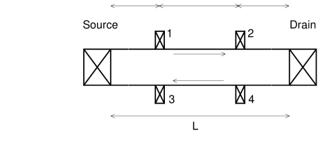
Figure 1: Geometry of the sample. Two identical layers are stacked vertically. The leads (source, drain, 1, 2, 3, and 4) can contact both layers or either layer. The drift directions along the edges are indicated by arrows. The lengths $L$, $a$, and $b$ specify the length of the sample and the positions of the leads.

2 Resistance

We consider a Hall bar type sample shown in Fig.1. The energy levels in the bulk are aligned in the two layers, and we consider the system in the lowest quantum Hall regime. For a single layer system the quantum Hall effect can be understood as a consequence of the spatial separation between left-going and right-going states on opposite edges of the sample.[4] At each edge we can define the chemical potential, which stays constant between the leads, and which differs between the opposite edges. However, in the case of a double layered system with finite inter-layer tunneling, the local chemical potential in each layer is generally not constant between the leads. We take $x$-axis along the edge and introduce $\mu_{\sigma}(x)$ for the local chemical potential, where $\sigma=\pm$ represents the layer index. Then the following equation governs the development of the chemical potentials between the leads:

$$\frac{d\mu_{\sigma}(x)}{dx}=-\frac{1}{\xi}[\mu_{\sigma}(x)-\mu_{-\sigma}(x)],$$ (1)

where $\xi$ is a parameter meaning the relaxation length for interedge equilibration. The current along an edge in layer $\sigma$ at position $x$ is given by

$$I_{\sigma}(x)=\frac{e}{h}[\mu_{\sigma}(x)-\epsilon_{0}],$$ (2)

with $\epsilon_{0}$ being a reference energy. The voltage leads will not affect the chemical potential, since the current will not flow through the lead. On the other hand the current leads give discontinuous change to the chemical potential. Following these rules we can solve for the chemical potentials of both layers, once the external current through each leads are given for any configuration of the leads.

As an example of such a solution, the followings are the obtained resistances for the case where only the minus layer has leads attached. Here current is fed to the minus layer through the source and extracted through the drain, and $\mu_{-}$ is observed at voltage leads 1 to 4 (see Fig.1). The longitudinal resistance $R_{xx}=R_{12}=R_{34}$ and the Hall resistance $R_{xy}=R_{13}$ are given as follows:

$$R_{xx}=\frac{h}{e^{2}}\frac{\exp(-2a/\xi)[1-\exp(-2b/\xi)]}{2[1+\exp(-2L/\xi)]},$$ (3)

$$R_{xy}=\frac{h}{e^{2}}\frac{1+\exp(-2a/\xi)+\exp[-2(L-a)/\xi]+\exp(-2L/\xi)}{2[1+\exp(-2L/\xi)]}.$$ (4)

where $a$ and $b$ specify the voltage probe positions as indicated in Fig. 1. Thus only in the strong (weak) coupling limit, where $L/\xi=\infty(0)$, the resistances are quantized: $R_{xx}=0$ and $R_{xy}=h/2e^{2}(h/e^{2})$.

3 Relaxation length $\xi$

The results for the resistances depend on the ratio $L/\xi$. Thus we need to know typical size of this parameter, and how it depends on various factors. The tunneling between the layers occur between state with the same energy. Let’s assume such pair of states are given by wave functions $\phi_{\sigma}(x,y,x)$ in the absence of tunneling. When the two edges of the two layers are aligned perfectly, they satisfy $\phi_{+}(x,y,z)=\phi_{-}(x,y,z-d)$, where $d$ is the interlayer separation. In the presence of the tunneling, they couple each other, and symmetric and antisymmetric combination of these states will become the eigen states. From the energy difference of these states, $\Delta_{SAS}$, the correlation length is estimated to be $\xi=\hbar v/\Delta_{SAS}$, where $v\simeq\ell\omega_{c}$ is the velocity of edge states, with $\ell$ being the magnetic length and $\omega_{c}$ being the cyclotron frequency. This estimate gives $L/\xi\simeq 50$ for $L=200\mu$m, and $\Delta_{SAS}=0.02$meV, which are typical values for an experimental situation. [2] This value of $L/\xi$ is quite large, and the system can be considered to be in the strong coupling regime. However, various factors reduce this value. Among them here we consider misalignment of the edges and in-plane magnetic field. We assume the center coordinate of $\phi_{+}$ projected on to the $xy$-plane cross many times with that of $\phi_{-}$. Among those crossings we focus on one of them, approximate the trajectory of the center coordinates around the crossing by straight lines, and calculate the contribution to the tunneling amplitude from a section of length $L_{s}(\gg\ell)$ around the crossing. We take the coordinate such that the $x$-axis bisects the two edges, so the two edges make angle $\pm\theta/2$ from the $x$-axis. The in-plane field $B_{x}$ and $B_{y}$ also refer to this coordinate. The tunneling amplitude, $I(B_{x},B_{y},\theta)$, is proportional to the overlap integral of $\phi_{+}$ and $\phi_{-}$. If we approximate $\phi_{\sigma}$ by the lowest Landau level wave function, the relative amplitude at $\theta=0$ is given as follows:

$${{I(B_{x},B_{y},0)}\over{I(0,0,0)}}={{2\ell}\over{L_{s}}}~{}{{\sin(L_{s}\beta_{y}/2\ell)}\over{\beta_{y}}}\exp(-{{\beta_{x}^{2}}\over{4}}),$$ (5)

where $\beta_{x}=B_{x}d/B_{z}\ell$, and $\beta_{y}=B_{y}d/B_{z}\ell$. So in this case, $B_{y}$ has a drastic effect: the amplitude is deminished by a small $B_{y}$, but $B_{x}$ dependence is small. For $\theta\gg(\ell/L_{s})^{2}$ the amplitude is much reduced and given by

$${{I(B_{x},B_{y},\theta)}\over{I(0,0,0)}}={{\ell}\over{L_{s}}}~{}\sqrt{{{2\pi}\over{\sin\theta}}}\exp[-{{(\beta_{x}^{2}+\beta_{y}^{2})}\over{4}}].$$ (6)

In this case $I(B_{x},B_{y},\theta)\ll I(0,0,0)$, and the effect of the in-plane magnetic field is quite weak.

4 Discussion

In recent experiments Ohno et al. [2] observed $R_{xy}\simeq h/e^{2}$ in the presence of finite $R_{xx}$ in the situation considered in Sec.2. This result is at a first glance inconsistent with our result, since $L/\xi\simeq 50$, if estimated using $\Delta_{SAS}=0.02$meV. However, the inconsistency is resolved, if the edges are not aligned perfectly. In this case the tunneling amplitude is reduced as shown in Eq. 6. In the experiments they observed that the effect of in-plane field is quite small. This insensitivity to the tilting is also in accordance with Eq. 6. Thus our theory is consistent with the experiments. It is general enough to treat various other configurations of leads. We hope such situations are realized experimentally, and results are compared with our theory.

References

References

- [1] J.P. Eisenstein, L.N. Pfeiffer, and K.W. West, Appl. Phys. Lett. 57, 2324 (1990).
- [2] Y. Ohno and H. Sakaki, Surf. Sci. (to be published), and Y. Ohno, M. Foley, and H. Sakaki, unpublished.
- [3] D. Yoshioka and A.H. MacDonald, Phys. Rev. B 53, 16168 (1996)
- [4] M. Büttiker, Phys. Rev. B 38, 9375 (1988).