Averaged Methods for Vortex-String Evolution

Abstract

We discuss friction-dominated vortex-string evolution using a new analytic model recently developed by the authors. By treating the average string velocity, as well as the characteristic lengthscale, as dynamical variables, we can provide a quantitative picture of the complete evolution of a vortex-string network. Previously known scaling laws are confirmed, and new quantitative predictions regarding loop production and evolution are made.

I Introduction

The concept of symmetry breaking plays a crucial role in modern physics, and one of its most interesting consequences is the formation of topological defects. These defects have been observed and studied in a wide variety of condensed matter contexts, including metal crystallization[1], liquid crystals[2, 3], superfluid helium[4, 5] and superconductors[6]. In models where they are allowed, defects will form whenever the rate of the phase transition is fast relative to the scale of the system size (in other words, a ‘quench’).

On the other hand, they are also believed to have formed in the early universe, and they can play an extremely important part in its evolution[7]. In this context, the conditions for their formation were first established by Kibble[8]—except for some subtleties in the case of the breaking of a gauge symmetry[9], they are entirely analogous.

The scaling evolution of vortex-string networks has been extensively studied analytically in both condensed matter and cosmological settings[10, 11, 12], but using rather different methods. This difference is perhaps understandable given the extremity of these two physical regimes, but it may not be necessary. Condensed matter descriptions tend to focus on a coarse-grained order parameter $\phi$, providing a low-level picture of defect motion by estimating energy dissipation rates. On the other hand, high energy physicists take an ‘idealized’ one-dimensional view of string dynamics by integrating out the radial degrees of freedom (in the Higgs $\phi$ and other fields) to obtain a low-energy effective action—the Nambu action. The resulting relativistic equations of motion can then be averaged to describe the large-scale evolution of the string network. Naturally one should also account for energy loss mechanisms, such as loop production—something that is not done in condensed-matter contexts.

The analytical study of cosmological string networks was started one decade ago by Kibble’s ‘one-scale’ model[10] (later modified by Bennett[13] and Albrecht & Turok[14]). There it was assumed that the evolution of the long-string network could be described by a single lengthscale, which is usually called the ‘correlation length’. One then supposes that a scaling solution exists at late times and ends up showing that such a solution will in fact exist and be stable subject to conditions on the loop production mechanisms. One of the caveats of this model is that it is only valid in the latter evolutionary stages when strings are moving relativistically. However, at early times the string dynamics is friction-dominated, due to particle–string scattering. Of course, this is also the relevant case in condensed matter physics.

A model of string evolution including the effects of frictional forces has been recently proposed by the authors[15, 16]. It is a simple generalization of the ‘one-scale’ model in which the average string rms velocity becomes a dynamical variable. This simple model provides the first quantitative description of the complete evolution of a string network in the early universe[15, 16]. In this paper, we will use it to study string evolution at constant temperature, which is relevant in condensed matter contexts. The main advantage of this approach is that one can easily account for the production and evolution of string loops. Although it should be seen as the basis for further work, the model is already predictive enough to be testable in laboratory experiments.

The structure of this paper is as follows. In the next section, after a review of string dynamics, the evolution equations for the ‘characteristic lengthscale’ and the average velocity of the long string network and each individual loop are derived and justified. The cases of strings arising from the breaking of gauge and global symmetries are both considered. The validity of these ‘averaged’ evolution equations is then tested against a simple—but physically relevant—loop solution in section 3. In section 4 we describe string evolution at constant temperature. The case where the dynamics is friction-dominated is directly applicable to a whole range of situations in condensed-matter systems. It will be shown that this model can easily reproduce some well-known results, notably the $L\propto t^{1/2}$ law. Furthermore, new quantitative predictions regarding loop evolution are made. We also discuss the opposite limit, where strings are initially ‘free’ and find that in that case a network quickly evolves towards the previous regime. We note that the evolution equations for the string network and the string loops are relatively straightforward, but the intervening derivation is not. First-time readers may wish to skip straight to the results in section IV.

II The averaged evolution equations

A Basics of string dynamics

The usual condensed matter approach to vortex dynamics is based on a ‘coarse-grained’ complex scalar field $\phi$. In quantum field theory, for example, one can consider the abelian-Higgs model, which is a relativistic generalization of the Ginzburg-Landau theory of superconductivity. It is also of interest to consider the global version of this, that is the Goldstone model.

In high-energy physics it also proves to be convenient to adopt a one-dimensional view of string dynamics (see [7] for a detailed discussion of the issues below). In this description a string sweeps out a two-dimensional surface (the worldsheet) which can be described by two ‘worldsheet coordinates’—one is time-like and can in fact be identified with the background time (which we will denote by $t$), while the other is space-like and simply labels points along the string (we will call it $\sigma$).

This one-dimensional description is essentially acheived by integrating over the radial modes of the vortex solution on the assumption that the scale of perturbations along the string is much larger than its width—thereby obtaining a low-energy effective action. For the case of a gauge (global) string, one thereby obtains the Nambu (Kalb-Ramond) action from the abelian-Higgs (Goldstone) model. Note that in the global case there are long range forces between the strings, in general there can be both external and self-field contributions to this. However, it can be shown (again, see [7] for a detailed discussion) that the later can be ‘renormalized out’, yielding the well-known logarithmically divergent string energy per unit length $\mu$ (which is a constant for gauge strings). By varying these actions it is then straightforward to obtain the string equations of motion.

There is, however, a crucial ingredient for string evolution missing. Since strings move through a background fluid, their motion is retarded by particle scattering. Vilenkin has shown[17] that this effect can be described by a frictional force per unit length that can be written

$${\bf F}_{\rm f}=-\frac{\mu}{\Gamma}\gamma{\bf v}\,,$$ (1)

where ${\bf v}$ is the string velocity, $\gamma$ is the Lorentz factor and $\Gamma$ is a constant damping coefficient, that can be written as the square of a characteristic propagation speed (which need not necessarily be the speed of light) times a ‘friction timescale’ $\tau_{\rm f}$, whose explicit value depends on the type of symmetry involved. For a gauge string, the main contribution comes from Aharonov-Bohm scattering[18], while in the global case it comes from Everett scattering[19]. For example, if the background fluid is a perfect gas, we have

$$\tau_{\rm f}=\left\{\begin{array}[]{ll}\frac{2\pi\hbar}{\beta}\frac{(k_{B}T_{c})^{2}}{(k_{B}T)^{3}}&\mbox{Gauge}\\ \frac{2\pi\hbar}{\beta}\frac{(k_{B}T_{c})^{2}}{(k_{B}T)^{3}}\ln\left(\frac{R}{\delta}\right)\ln^{2}(T\delta)&\mbox{Global}\end{array}\right.$$ (2)

where $T$ is the background temperature and $\beta$ is a numerical factor related to the number of particle species interacting with the string (strictly speaking, its value is slightly different in the two cases, but a common symbol will be used for simplicity). It should also be noted that the Everett scattering formula is only valid when the particle wavelength is much larger than the string thickness $\delta$. Alternatively, $\Gamma$ can be written as the characteristic propagation speed times a ‘friction lengthscale’ $\ell_{\rm f}$.

For string motion in a flat background, the string equations of motion with the frictional force (1) can then be written as[16]

$$\frac{1}{c^{2}}{\ddot{\bf x}}+\left(1-\frac{{\dot{\bf x}}^{2}}{c^{2}}\right)\frac{\dot{\bf x}}{\Gamma}=\frac{1}{\epsilon}\left(\frac{{\bf x}^{\prime}}{\epsilon}\right)^{\prime}\,,$$ (3)

$${\dot{\epsilon}}+\frac{{\dot{\bf x}}^{2}}{\Gamma}\epsilon=0\,,$$ (4)

where the dimensionless parameter $\epsilon$ (which can be interpreted as a ‘coordinate energy per unit length’) is defined by

$${\epsilon^{2}=}\frac{{{\bf x}^{\prime}}^{2}}{{1-{\dot{\bf x}}^{2}/c^{2}}}\,,$$ (5)

and dots and primes respectively denote time and space derivatives. This form of the evolution equations proves to be particularly useful because dissipation is naturally incorporated in the decay of the coordinate energy density $\epsilon$, while preserving the gauge conditions. Note that while this is a truly relativistic formalism, it is straightforward to obtain the non-relativistic limit that will be adequate to condensed matter contexts where the dynamics is friction-dominated. In this case, Eqns. (3-5) reduce to

$$\frac{{\dot{\bf x}}}{\Gamma}=-\frac{1}{{{\bf x}^{\prime}}^{4}}\left[{\bf x}^{\prime}\wedge\left({\bf x}^{\prime}\wedge{\bf x}^{\prime\prime}\right)\right]\,,$$ (6)

and one can recognize the right-hand side as the friction force term (which is dominant in this limit), e.g. on a superfluid vortex[20]

Incidentally, it has been shown[21] that a global string will behave as a superfluid vortex if it is introduced in a homogeneous background (with a density $\rho_{h}$, say)—physically, this corresponds to giving it angular momentum. The interaction between this background and the string originates an additional force, known as the (relativistic) Magnus force, and (3) becomes

$$\frac{1}{c^{2}}{\ddot{\bf x}}+\left(1-\frac{{\dot{\bf x}}^{2}}{c^{2}}\right)\frac{\dot{\bf x}}{\Gamma}=\frac{1}{\epsilon}\left(\frac{{\bf x}^{\prime}}{\epsilon}\right)^{\prime}+\Gamma^{\prime}\dot{\bf x}\wedge\frac{{\bf x}^{\prime}}{\epsilon}\,,$$ (7)

where $\Gamma^{\prime}\propto\rho_{h}^{1/2}$; note that (4) remains unchanged.

B Lengthscale evolution

We can now proceed to average the string equations of motion to describe the large-scale evolution of the string network. We therefore define the total string energy and the average rms string velocity to be

$$E=\mu\int\epsilon d\sigma\,,$$ (8)

$$v^{2}\equiv\langle{\dot{\bf x}}^{2}\rangle=\frac{{\int{\dot{\bf x}}^{2}\epsilon d\sigma}}{{\int\epsilon d\sigma}}\,.$$ (9)

Differentiating (8) and using (4) and (9), we see that the total string energy density will obey the following evolution equation:

$$\frac{d\rho}{dt}+\frac{v^{2}}{\Gamma}\rho=0\,.$$ (10)

This includes both long strings and loops which have a low probability of interacting with other strings before decaying. We shall study the evolution of the long-string network on the assumption that it can be characterized by a single lengthscale $L$; this can be interpreted as the inter-string distance or the ‘correlation length’. Strings larger than $L$ will be called long or ‘infinite’; otherwise they will be called loops. For Brownian long strings, we can define the ‘correlation length’ $L$ in terms of the network density $\rho_{\infty}$ as

$$\rho_{\infty}\equiv\frac{\mu}{L^{2}}\,.$$ (11)

Following Kibble[10], the rate of loop production from long-string collisions can be estimated as follows. Conceptually, we divide the network into a collection of segments of length $L$, each in a volume $L^{3}$. Consider another segment of length $l$ moving with a velocity $v_{\infty}$; the probability of it encountering one of the other segments within a time $\delta t$ is approximately $lv_{\infty}\delta t/L^{2}$. Consistently with our ‘one-scale’ assumption, we then assume that the probability of such an intersection creating a loop of length in the range $l$ to $l+dl$ will be given by a scale-invariant function $w\left({l/L}\right)$. The rate of energy loss into loops is then given by

$$\left(\frac{d\rho_{\infty}}{dt}\right)_{\rm to\ loops}=\rho_{\infty}\frac{v_{\infty}}{L}\int w\left(\frac{\ell}{L}\right)\frac{\ell}{L}\frac{d\ell}{L}\equiv{\tilde{c}}v_{\infty}\frac{\rho_{\infty}}{L}\,.$$ (12)

where the loop ‘chopping’ efficiency ${\tilde{c}}$ is assumed to be constant. By subtracting the loop energy losses (12) from (10) and then using (11), we obtain the overall evolution equation for the characteristic lengthscale $L$,

$$2\frac{dL}{dt}=\frac{v_{\infty}^{2}}{\Gamma}L+{\tilde{c}}v_{\infty}\,.$$ (13)

C Loop evolution

The main advantage of the present approach is that we can also study the evolution of the loop density and distribution, which have so far been neglected in the condensed matter literature. The traditional approach in cosmology is to define $n_{\ell}(\ell,t)d\ell$ to be the number density of loops with length in the range $(\ell,\ell+d\ell)$ at time $t$; the corresponding loop energy density distribution is

$$\rho_{\ell}(\ell,t)d\ell=\mu\ell n_{\ell}(\ell,t)d\ell\,.$$ (14)

Note that the total loop energy density is

$$\rho_{o}\equiv\int\rho_{\ell}(\ell,t)d\ell\,,$$ (15)

and $\rho=\rho_{\infty}+\rho_{o}$ From our assumptions on the loop production rate (12) it is then easy to see that

$$\frac{d\rho_{\ell}}{dt}+\frac{v_{\ell}^{2}}{\Gamma}\rho_{\ell}=\mu\frac{v_{\infty}\ell}{L^{5}}w\left(\frac{\ell}{L}\right)\,.$$ (16)

However, note that this equation is ‘static’, in the sense that it does not include loop decay mechanisms.

Instead, we start by using our analytic model to describe the evolution of each individual loop. Knowing the energy density transferred from long strings into loops and estimating their sizes at formation (see below), one can determine the energy density in loops and other relevant quantities at all times. This formalism does not allow for possible loop reconnections or self-intersections but these should not be important in a friction-dominated regime.

The physical size of a loop is simply given by

$$\ell=\int_{loop}\epsilon d\sigma\,,$$ (17)

and its time evolution is easily found to be

$$\frac{d\ell}{dt}=-\ell\frac{v^{2}_{\ell}}{\Gamma}\,.$$ (18)

Now, we will assume that loop production is ‘monochromatic’, ie that loops formed at a time $t_{p}$ have an initial length

$$\ell(t_{p})=\alpha(t_{p})\ L(t_{p})\,,$$ (19)

where $\alpha$ is a parameter of order unity.

With this ansatz the scale-invariant loop production function $w$ (see (12)) becomes

$$w\left(\frac{\ell}{L}\right)=\frac{{\tilde{c}}}{\alpha}\delta\left(\frac{\ell}{L}-\alpha\right)\,,$$ (20)

and the rate of energy loss into loops becomes

$$\left(\frac{d\rho_{\infty}}{dt}\right)_{\rm to\ loops}=\mu{\tilde{c}}\frac{v_{\infty}}{L^{3}}\,.$$ (21)

Hence the energy density converted into loops from time $t$ to $t+dt$ is

$$d\rho_{o}(t)=\mu{\tilde{c}}\frac{v_{\infty}}{L^{3}}dt\,;$$ (22)

this corresponds to a fraction

$$\frac{d\rho_{o}(t)}{\rho_{\infty}(t)}={\tilde{c}}\frac{v_{\infty}}{L}dt\,,$$ (23)

of the energy density in the form of long strings at time $t$. Then using our ansatz (20), the corresponding number of loops produced in a volume $V$ is

$$dN(t)=\frac{{\tilde{c}}}{\alpha}\frac{v_{\infty}}{L^{4}}Vdt\,;$$ (24)

hence the ratio of the energy densities in loops and long strings at time $t$ is (neglecting the initial loop population at $t=t_{c}$)

$$\varrho(t)\equiv\frac{\rho_{o}(t)}{\rho_{\infty}(t)}=L^{2}(t)\int_{t_{c}}^{t}\frac{dN(t^{\prime})\ell(t,t^{\prime})}{V}={\tilde{c}}L^{2}(t)\int_{t_{c}}^{t}\frac{v_{\infty}(t^{\prime})}{L^{4}(t^{\prime})}\frac{\ell(t,t^{\prime})}{\alpha(t^{\prime})}dt^{\prime}\,,$$ (25)

where $t_{c}$ is the moment of the network formation and $\ell(t,t^{\prime})$ is the length at time $t$ of loops produced at time $t^{\prime}$.

We can therefore numerically (and, in some simple limit cases, analytically) determine the loop density at all times. This generalized ‘one-scale’ model can therefore provide a complete description of a string network.

D Velocity evolution

We now consider the evolution of the average string velocity $v$. A non-relativistic equation can be easily obtained: it is just Newton’s law,

$$\frac{\mu}{c^{2}}\frac{dv}{dt}=\frac{\mu}{R}-\mu\frac{v}{\Gamma}\,.$$ (26)

This merely states that curvature accelerates the strings while friction slows them down. On dimensional grounds, the force per unit length due to curvature should be $\mu$ over the curvature radius $R$. The form of the damping force can be found similarly.

A relativistic generalization of the velocity evolution equation (26) can be obtained more rigorously by differentiating (9):

$$\frac{1}{c^{2}}\frac{dv}{dt}=\left(1-\frac{v^{2}}{c^{2}}\right)\left(\frac{k}{R}-\frac{v}{\Gamma}\right)\,.$$ (27)

This is exact up to second-order terms. In the curvature term, we have introduced $R$ via the definition of the curvature radius vector,

$$\frac{\hat{\bf u}}{R}=\frac{d^{2}{\bf x}}{ds^{2}}\,,$$ (28)

where $\hat{\bf u}$ is a unit vector and $s$ is the physical length along the string (related to the coordinate length $\sigma$ by $ds=|{\bf x}^{\prime}|d\sigma=\left(1-{\dot{\bf x}}^{2}/c^{2}\right)^{1/2}\epsilon d\sigma$). The dimensionless parameter $k$ is defined by

$$\langle(1-\frac{{\dot{\bf x}}^{2}}{c^{2}})({\dot{\bf x}}\cdot\hat{\bf u})\rangle\equiv kv\left(1-\frac{v^{2}}{c^{2}}\right)\,.$$ (29)

Note that in the case of long strings, our ‘one-scale’ assumption implies that the curvature radius coincides with the correlation length, $R\equiv L$; on the other hand, for a loop of size $\ell$ we should have $\ell\approx 2\pi R$.

The parameter $k$ is ‘phenomenological’, and is related to the presence of small-scale ‘wiggles’ on strings: on a perfectly smooth string, $\hat{\bf u}$ and ${\dot{\bf x}}$ will be parallel so $k=1$ (up to a second-order term as above); however this need not be so for a wiggly string[16]. On the other hand, one can show that in flat spacetime (with no friction) $k=0$.

In the case of long strings, we should expect $k=1$ since the correlation length $L$ is much larger than the ‘friction length’ $\ell_{\rm f}$. Now, consider a particular string loop. While it is large compared with the friction lenghtscale, taking $k\approx 1$ should again be a good assumption. In the opposite limit friction is no longer effective in damping its motion, and it moves as if it was in flat spacetime. Thus one requires that $k\rightarrow 0$ as $R\rightarrow 0$. In particular, demanding that their limiting velocity be $v^{2}_{\ell}/c^{2}=1/2$ leads to the requirement that $k\propto R$ as $R\rightarrow 0$. With these requirements in mind, and after comparing with the ‘microscopic’ (ie, unaveraged) evolution of some simple solutions (to be described in the next section) one arrives at the following ansatz:

$$k=\left\{\begin{array}[]{ll}1\,,&\mbox{$\frac{R}{\ell_{\rm f}}>\chi$}\\ \frac{1}{\sqrt{2}}\frac{R}{\ell_{\rm f}}\,,&\mbox{$\frac{R}{\ell_{\rm f}}<\chi$}\end{array}\right.$$ (30)

where $\chi$ is a numerical coefficient[22] of order one. Recall that the physical loop length is approximately $\ell=2\pi R$, while for the long-string network $L=R$.

Equations (13), (18) and (27) form the basis of our generalized ‘one-scale’ model, which we will now proceed to apply.

III ‘Averaged’ versus ‘microscopic’ evolution

In order to check the validity of our ‘averaged’ evolution model, and in particular our ansatz for $k$, we will test it against a simple loop solution.

Consider a circular loop in a flat background with a constant friction timescale—that is, a condensed-matter-like situation. We can describe the loop trajectory simply by

$${\bf x}=r(t)(\sin\theta,\cos\theta,0)\,,\,\theta\in[0,2\pi]\,.$$ (31)

Then equations (3,4) reduce to

$$\frac{1}{c^{2}}{\ddot{r}}+(1-\frac{{\dot{r}}^{2}}{c^{2}})\left(\frac{{\dot{r}}}{\Gamma}+\frac{1}{r}\right)=0\,.$$ (32)

Note that the physical (‘invariant’) loop radius is $R=r/\sqrt{1-{\dot{r}}^{2}/c^{2}}$, obeying

$${\dot{R}}=-R\frac{{\dot{r}}^{2}}{\Gamma}\,;$$ (33)

also the ‘microscopic’ velocity is $v=-{\dot{r}}$ and obeys

$$\frac{1}{c^{2}}{\dot{v}}=\left(1-\frac{v^{2}}{c^{2}}\right)\left(\frac{1}{r}-\frac{v}{\Gamma}\right)\,.$$ (34)

On the other hand, our averaged evolution equations (18,27) take the form

$$\frac{d{\bar{R}}}{dt}=-{\bar{R}}\frac{{\bar{v}}^{2}}{\Gamma}\,,$$ (35)

$$\frac{1}{c^{2}}\frac{d{\bar{v}}}{dt}=\left(1-\frac{{\bar{v}}^{2}}{c^{2}}\right)\left(\frac{k({\bar{R}})}{{\bar{R}}}-\frac{{\bar{v}}}{\Gamma}\right)\,.$$ (36)

Notice the similarity between the two approaches. Loops with size much larger than a ‘friction lengthscale’ that can be defined in the obvious way from the friction timescale will be overdamped, with the velocity being approximately given by

$$v\sim\frac{\Gamma}{r}\,.$$ (37)

In this case the two sets of evolution equations actually coincide—hence justifying our $k=1$ ansatz for large R. As the loop gains velocity $r$ and $R$ become significantly different and this equivalence ceases to be valid. When $R$ becomes much smaller than $\ell_{\rm f}$, the loop still looses energy due to friction, but this is no longer effective in damping its motion—the loop now begins to oscillate relativistically. In particular, over one ‘period’ $v$ oscillates between $0$ and $1$. But we know that the averaged velocity should (in the limit) be ${\bar{v}}^{2}/c^{2}=1/2$; this is the physical reason why we need a ‘phenomenological’ varying $k$ on small scales. As we mentioned previously, this requirement fixes the behaviour of $k$ on small scales to be as shown in (30). The remaining question is then how to match the two regimes.

First of all, we need a clear idea of when (and where) the transition occurs. A good guess would be the moment of the ‘first collapse’, ie, the moment when we first have $v=c$. In fact, this turns out to be a well-defined event. As was first pointed out by Garriga and Sakellariadou[22] (and can be easily seen by analytical or numerical study of the equation of motion (32)), circular loops with initial radius much larger than the friction length always reach $v=c$ for the first time when

$$\left(\frac{R}{\ell_{\rm f}}\right)_{col}=\chi_{c}\simeq 0.5691\,.$$ (38)

Note that $r_{i}\gg\ell_{\rm f}$ is the physically relevant case for string dynamics in condensed matter contexts (recall that the dynamics in that case is always friction-dominated). Also note that because of friction, all loops will rapidly become (almost) circular.

After numerically comparing the averaged and microscopic evolution equations, we find that the simplest possibility,

$$k=\left\{\begin{array}[]{ll}1\,,&\mbox{$\frac{R}{\ell_{\rm f}}>\chi$}\\ \frac{1}{\sqrt{2}}\frac{R}{\ell_{\rm f}}\,,&\mbox{$\frac{R}{\ell_{\rm f}}<\chi$}\end{array}\right.$$ (39)

(see figure 1) provides the best answer (see figures 2,3). In particular, this turns out to be significantly better than assuming smoother (and slower) transitions between the two regimes. As can be readily seen, this ansatz provides a very good fit, considering the lack of parameters available.

In passing, it is worth pointing out that one can also easily calculate the loop lifetime[22]. In the relativistic regime, the ${\bar{R}}$ evolution equation can be written

$$\frac{d{\bar{R}}}{dt}=-\frac{{\bar{R}}}{\tau_{\rm f}}\,,$$ (40)

so we can immediately estimate that the loop will disappear in a time $t_{dec}\sim 2\tau_{\rm f}$ after its first collapse.

Having thus established, in a simple but physically relevant case, the validity of our generalized ‘one-scale model’, and in particular of the ansatz for $k$, we now proceed to apply it to the study of string evolution in condensed matter contexts.

IV String evolution at constant temperature

A The condensed-matter context

1 Network scaling

As we already noted, in this case the dynamics is always dominated by friction. This means that the ‘correlation length’ $L$ should always be larger than the (constant) friction length, so we can take $k=1$. Then the evolution equations can be approximated by

$$2\frac{dL}{dt}=L\frac{v^{2}}{\Gamma}+{\tilde{c}}v\,,$$ (41)

$$\frac{dv}{dt}=c^{2}\left(\frac{1}{L}-\frac{v}{\Gamma}\right)\,;$$ (42)

the friction lengthscale and the string energy per unit length being respectively

$$\ell_{\rm f}=\left\{\begin{array}[]{ll}s&\mbox{Gauge}\\ s\ln\left(\frac{L}{\delta}\right)&\mbox{Global}\end{array}\right.$$ (43)

and

$$\mu=\left\{\begin{array}[]{ll}T_{c}^{2}&\mbox{Gauge}\\ T_{c}^{2}\ln\left(\frac{L}{\delta}\right)&\mbox{Global}\end{array}\right.$$ (44)

where $T_{c}$ is the temperature at which the strings form and $s$ is a constant. We then find the following late-time asymptotic behaviour:

$$L=\sqrt{1+{\tilde{c}}}\left(\Gamma t\right)^{1/2}\,,$$ (45)

$$v=\frac{\Gamma}{L}\,.$$ (46)

Note that in both cases the asymptotic behaviour of the long-string density is

$$\rho_{\infty}=\frac{(k_{B}T_{c})^{2}}{(1+{\tilde{c}})\hbar sc^{2}t}\,;$$ (47)

the extra logarithmic dependencies in the global case cancel out. It should be emphasized that in condensed-matter analyses one does not consider loop formation, although there is experimental[2] and computational evidence for them. Our results show that loop formation can play an important evolutionary role. The asymptotic ratio of the loop production and friction terms is a constant, which is precisely ${\tilde{c}}$—which in this way acquires a clearer physical meaning. As expected, increasing ${\tilde{c}}$ (or including loop losses in the first place) leads to a lower network scaling density and a smaller average velocity $v$; furthermore, the approach to the scaling regime is also faster.

Figure 4 illustrates the relaxation to scaling of a network of gauge strings for a particular set of initial conditions, with and without loop production. The differences between the two cases are clearly visible. Notice that in the gauge case the temperature only enters the scaling solution in the prefactor $s$; hence the plots of figure 4 (where the dimensionless variable $L/s$ is used) are ‘universal curves’, that is, hold for all relevant temperatures.

In the global case, the logarithmic dependence of the friction lengthscale gives rise to an additional logarithmic dependence of the scaling solution on temperature. One can define $d$ via $L/\delta\equiv L/sd$; in the Goldstone model we then have

$$d^{-1}(T)=\sqrt{\frac{\lambda}{6}}\left(\frac{T_{c}}{T}\right)^{3}\ln^{2}\left(\sqrt{\frac{\lambda}{6}}\frac{T}{T_{c}}\right)\,.$$ (48)

The approach to scaling of a network of global strings is shown in figure 5 for two different temperatures. Note the enhancement of loop production at the early stages, since the string velocity is high; correspondingly, there is a fast growth of the correlation length. Comparing with the gauge case (see figure 4), one finds that the effect of the extra logarithmic terms is significant for at least three orders of magnitude in time.

2 Loop populations

Now let us consider the loop populations. In the traditional (that is, ‘static’) approach one would simply calculate the loop distribution $\rho_{\ell}(\ell,t)$ in the scaling regime—which we assume starts at some time $t_{s}$. The corresponding evolution equation is then

$$\frac{d\rho_{\ell}}{dt}+\frac{v^{2}_{\ell}}{\Gamma}\rho_{\ell}=g\mu\frac{v\ell}{L^{5}}w\left(\frac{\ell}{L}\right)\,.$$ (49)

Since the loop size and velocity are initially (that is, while the loops are overcritically damped) slowly-varying quantities, this approach will only be accurate at the early stages of evolution of each lengthscale $\ell$. Afterwards $\ell$ and $v$ will vary quickly (the averaged $v$ will be a constant later), and in this situation this approach is no longer useful. Note that since friction is dominating the dynamics, irregularities are quickly erased and all loops become circular—hence the discussion of section 3 is particularly relevant here.

Consistent with what we found there, we will use the following simplifying ansatz

$$\frac{v_{\ell}(R,t)}{c}=\left\{\begin{array}[]{ll}\frac{\ell_{\rm f}}{R}&\mbox{$\frac{R}{\ell_{\rm f}}\geq\sqrt{2}$}\\ \frac{1}{\sqrt{2}}&\mbox{$\frac{R}{\ell_{\rm f}}\leq\sqrt{2}$}\end{array}\right.$$ (50)

(where $\ell=2\pi R$); naturally in this approach only the first case is relevant. Furthermore, the loop production parameter $\alpha$ (defined is (19)) should be a constant (we are considering a scaling regime) of order unity.

After some algebra, we find the following solution

$$\rho_{\ell}(\ell,t)=\left\{\begin{array}[]{ll}\frac{2g{\tilde{c}}\alpha^{2}\mu}{1+{\tilde{c}}}\ell^{-3}\exp{\left[-4\pi^{2}c\ell_{\rm f}t\left(\frac{1}{\ell^{2}}-\frac{1}{\alpha^{2}L^{2}}\right)\right]}&\mbox{$\alpha L_{s}<\ell<\alpha L$}\\ 0&\mbox{otherwise}\end{array}\right.$$ (51)

where we have neglected any loops present at time $t_{s}$. Note that in the global string case these expressions are only approximate, since there are additional logarithmic dependencies in the energy per unit length $\mu$ and the friction length $\ell_{\rm f}$.

However, we can do more than that. To begin with, we can determine the loop lifetime. During most of it the loop will have a length greater than the friction lenghtscale, so we can approximate their velocity by (50). Then its length will vary according to

$$\frac{d\ell}{dt}\approx-4\pi^{2}\frac{\Gamma}{\ell}\,,$$ (52)

so its lifetime is

$$\frac{\tau(\ell)}{\tau_{\rm f}}=\frac{1}{8\pi^{2}}\left(\frac{\ell}{\ell_{\rm f}}\right)^{2}\,.$$ (53)

Of course a more accurate result can be obtained numerically (see figure 6); for large enough loops we find

$$\frac{\tau(\ell)}{\tau_{\rm f}}=\iota\left(\frac{\ell}{\ell_{\rm f}}\right)^{2}\,,\,\iota\sim 0.0126\,,$$ (54)

showing our analytical estimate to be correct to within a fraction of one percent.

On the other hand, we can simply use (25) to determine the ratio of the energy densities in the form of loops and long strings. In this case, taking $\alpha\sim 1$, it simplifies to

$$\varrho(t)=\frac{\rho_{o}(t)}{\rho_{\infty}(t)}={\tilde{c}}L^{2}(t)\int_{t_{c}}^{t}\frac{v_{\infty}(t^{\prime})}{L^{4}(t^{\prime})}\ell(t,t^{\prime})dt^{\prime}\,.$$ (55)

In fact, an approximate analytic solution for $\varrho$ can be found in the scaling regime. We will assume that such a regime starts at a time $t_{s}$ and neglect any existing loops at $t_{s}$. The contribution of each loop to the loop density will only be significant while it overdamped. In this regime we can assume that its length is approximately constant, $\ell(t,t^{\prime})\sim\ell(t^{\prime})=L(t^{\prime})$ (hence we will be deriving an overestimate of $\varrho$). On the other hand, the end of this regime approximately coincides with the moment of loop decay, which according to (54) for a loop formed at time $t^{\prime}$ happens at

$$t\equiv\xi^{-1}t^{\prime}=\left[1+\iota(1+{\tilde{c}})\right]t^{\prime}\,,$$ (56)

for a loop formed at time $t^{\prime}$. Then we have

$$\ell(t,t^{\prime})=\left\{\begin{array}[]{ll}L(t^{\prime})&\mbox{$t^{\prime}\leq t\leq\xi t^{\prime}$}\\ 0&\mbox{otherwise}\end{array}\right.$$ (57)

and there are two corresponding cases to consider for the integral (55) (see figure 7), according to whether or not loops have decayed at the time in question,

$$\varrho(t)={\tilde{c}}L^{2}(t)\int_{f(t)}^{t}\frac{v_{\infty}(t^{\prime})}{L^{3}(t^{\prime})}dt^{\prime}\,,$$ (58)

where

$$f(t)=\left\{\begin{array}[]{ll}t_{s}&\mbox{$t\leq\xi^{-1}t_{s}$}\\ \xi t&\mbox{$t\geq\xi^{-1}t_{s}$}\end{array}\right.$$ (59)

We then obtain

$$\varrho_{scaling}=\left\{\begin{array}[]{ll}\frac{{\tilde{c}}}{1+{\tilde{c}}}\left(\frac{t}{t_{s}}-1\right)&\mbox{$t\leq\xi^{-1}t_{s}$}\\ \iota{\tilde{c}}&\mbox{$t\geq\xi^{-1}t_{s}$}\end{array}\right.$$ (60)

This is easily confirmed numerically. Figure 8 displays the evolution of the ratio of the loop and long string densities corresponding to the gauge string network of figure 4. In this case ${\tilde{c}}=1$, so our analytical estimate is $\varrho_{scaling}=0.0126$, while numerically we find $\varrho_{scaling}\sim 0.0089$. Notice that with our initial conditions the ratio of the energy densities in loops and long strings is larger while the network is approaching scaling than in the scaling regime. This is simply due to the fact that loops with initial sizes not much larger than the friction lengthscale live longer than predicted by (54) (as can be seen in figure 6).

Naturally, since we can find out how each loop evolves, it is always possible to find out how many loops there are at any time on any given length interval. Note that in this context reconnections and self-intersections should be negligible, at least when the loops are large compared to $\ell_{\rm f}$ (because they are non-relativistic)—which is when their contribution to the loop density is significant.

Furthermore, using the results from our discussion in section 2C, we easily find that the fraction of the energy density in long strings at time $t$ that is converted into loops in the time interval $\Delta t=\tau_{\rm f}$ is asymptotically

$$f_{\tau_{\rm f}}=\frac{{\tilde{c}}}{1+{\tilde{c}}}\frac{\tau_{\rm f}}{t}\,;$$ (61)

note that this is a very small number. Furthermore, note that as we increase ${\tilde{c}}$ there is a limiting fraction. Also, the number of loops formed in a time interval $\Delta t=\tau_{\rm f}$ and volume $\ell_{\rm f}^{3}$ is

$$n_{\tau_{\rm f}}=\frac{{\tilde{c}}}{(1+{\tilde{c}})^{3/2}}\left(\frac{\tau_{\rm f}}{t}\right)^{5/2}\,;$$ (62)

in this case, $n_{\tau_{\rm f}}$ goes to zero as ${\tilde{c}}$ grows—this is because $L$ and hence the loop size at formation grow with ${\tilde{c}}$.

3 Discussion

The $t^{1/2}$ scaling law for the characteristic lengthscale is a well-known result in the theory of phase ordering (that is, the growth of ‘order’—as measured by some correlation length—by domain coarsening when a system is ‘quenched’ from a homogeneous phase into a broken-symmetry phase) with a non-conserved order parameter. In this context it is usually called the Lifshitz-Allen-Cahn[23] growth law, and it is widely supported by simulations and experiment[24] (see also ref. [12] for a recent review). In the usual approach, one sets up a continuum description in terms of a coarse-grained order parameter $\phi$ and then assumes a scaling hypothesis, that is, that at late times there is a single lengthscale such that the domain structure is time-independent (in a statistical sense) when all lengths are rescaled by it. The growth law is usually derived by studying the dynamics of the defects in $\phi$ (see, for example, Section 3 in Bray’s review[12]). A recent alternative approach[25] proceeds instead by comparing the global rate of energy change due to the energy dissipation to the local evolution of the order parameter; with the scaling hypothesis, the time-dependence of the lengthscale can be determined self-consistently.

In particular, the $L\propto t^{1/2}$ law has been experimentally confirmed for the evolution of a string network in a nematic liquid crystal (roughly speaking, a liquid made of rod-like molecules)—eg, see ref. [2] where, as mentioned, loop formation and decay have been seen.

The $v\propto L^{-1}\ln L$ scaling law is also known in hydrodynamical contexts. Furthermore, it has been shown that it holds for superfluid vortex-rings[21] in the context of a modified Goldstone model (in a way described in the previous section). Hence the above result seems to indicate that a global string network at constant temperature asymptotically behaves as if it was made of loops of size $L$.

As we hopefully made clear, the above discussion of the loop lifetime and density is entirely new in this context. It is hoped that these results, obtained in a fairly simple way in this approach will stimulate condensed matter theoreticians an experimentalists…

Finally, in the case of superfluid vortices, despite the additional Magnus force term, the evolution equations also have the form (41,42). In this case, however, the physical meaning of the friction lengthscale is not clear. Furthermore, it is also not clear how one can describe the effect of the Magnus force on the evolution of the network. We hope to address these issues at a later stage.

Therefore, a model aimed at describing the evolution of cosmic strings[15, 16] can be straightforwardly applied to rather more ‘down-to-earth’ situations, with some advantages over previously existing analytical approaches (in particular, allowing a precise treatment of loop production). This is rather remarkable, considering the difference in the energy scales involved.

B The ‘relativistic’ regime

As a matter of completeness as well as mathematical curiosity, we now consider the evolution of a string network in flat space with a constant friction lengthscale when the initial conditions are such that the correlation length is much smaller than the friction lengthscale. This is therefore the opposite regime to that usually observed in condensed matter.

The evolution equations will now be

$$2\frac{dL}{dt}=\frac{v^{2}}{\Gamma}L+{\tilde{c}}v\,,$$ (63)

$$\frac{dv}{dt}=\left(c^{2}-v^{2}\right)\left(\frac{k(L)}{L}-\frac{v}{\Gamma}\right)\,,$$ (64)

where we will assume that our ansatz for $k$ for string loops also holds for long strings (see ref. [16] for a more complete discussion of this point), that is

$$k=\left\{\begin{array}[]{ll}1\,,&\mbox{$\frac{L}{\ell_{\rm f}}>\chi$}\\ \frac{1}{\sqrt{2}}\frac{L}{\ell_{\rm f}}\,,&\mbox{$\frac{L}{\ell_{\rm f}}<\chi$}\end{array}\right.$$ (65)

In the regime where $R\ll\ell_{\rm f}$ the $v$-equation is independent of $L$, so its particularly easy to find the scaling regime

$$\frac{L}{\ell_{\rm f}}=\left(\frac{L_{o}}{\ell_{\rm f}}+2\sqrt{2}{\tilde{c}}\right)\exp\left[\frac{c}{4\ell_{\rm f}}(t-t_{0})\right]-2\sqrt{2}{\tilde{c}}\,,$$ (66)

$$\frac{v}{c}=\frac{1}{\sqrt{2}}\,.$$ (67)

Hence $L$ grows exponentially fast and quickly ‘catches up’ with $\ell_{\rm f}$; in other words, a network starting in the ‘free’ regime rapidly evolves to the usual friction-dominated regime. Figure 9 displays the evolution of a gauge string network in the free regime, and in particular the transition to the damped regime. Note that if loop production is allowed, this fast growth of the correlation length will obviously mean that an extremely large number of loops is produced. In this case, the energy density in loops actually exceeds the energy in long strings—in the above plot, by a factor of $10^{4}$. A word of caution is however needed here. In this case, loop reconnections onto the long string network should play an important role. However, since we still get an exponential growth if loop production is switched off (${\tilde{c}}=0$)—although the growth rate of $L$ is obviously much larger for ${\tilde{c}}\not=0$—our results should at least be qualitatively correct.

V Conclusions

In this paper we have discussed the applicability in condensed matter contexts of a recently-developed model of string evolution[15, 16], where a ‘characteristic lengthscale’ and the average velocity are the dynamical variables. This has allowed us to properly describe friction-dominated string dynamics, hence providing the first complete and fully quantitative study of string networks and their corresponding loop populations in condensed matter (as well as cosmological[16]) contexts. The fact that these results can be obtained in a model initially aimed at describing cosmic string evolution is, of course, a manifestation of the universality of symmetry breaking and defect formation phenomena, but it also lends weight to the validity of this approach because these cosmological models have been extensively tested numerically.

We have confirmed two previously known condensed matter scaling laws, while noting the significant effects of loop production (which is not considered in standard approaches). We also presented the first (analytic or otherwise) discussion of the evolution of the overall loop density, while also determining loop lifetimes. As we have already stated, the literature on string loops in phase ordering kinetics appears to be restricted to a few references to the observation of loop production and decay in laboratory experiments[2]. It is hoped that these more quantitative predictions will trigger further efforts from the condensed matter community.

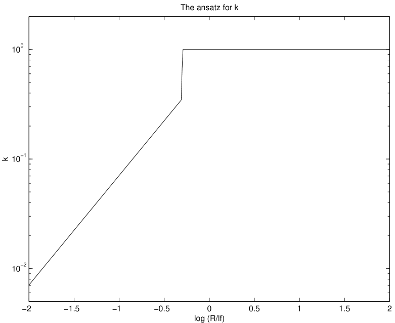
FIG. 1.: The ansatz for parameter $k$ for string loops in a condensed-matter context as a function of the rescaled loop radius. The behaviour at large and small scales has a physical justification (see text); matching was done numerically.

         

         

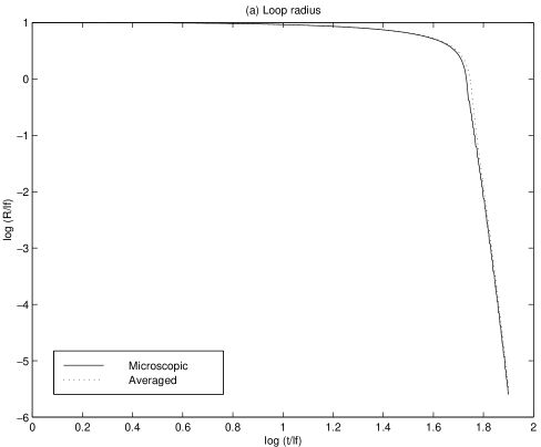
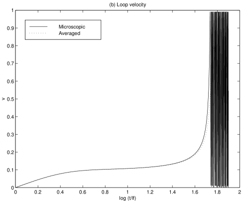
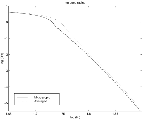
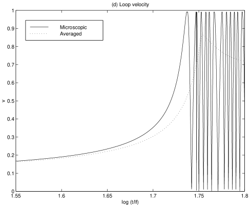
FIG. 2.: Comparing the ‘microscopic’ (solid lines) and ‘averaged’ (dashed) evolution equations for a circular loop in a condensed-matter context. Length and time are in units of $\ell_{\rm f}$, and the time axis is with a logarithmic scale. Plot (a) depicts the log of the (rescaled) radius, while (b) depicts the loop velocity (in units of $c$). The lower graphs are close-ups of the upper ones.

         

         

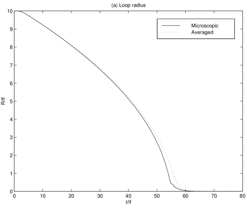
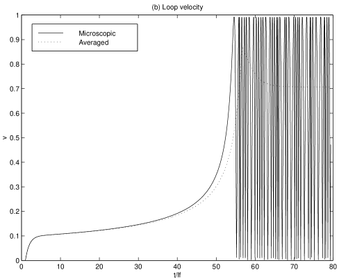
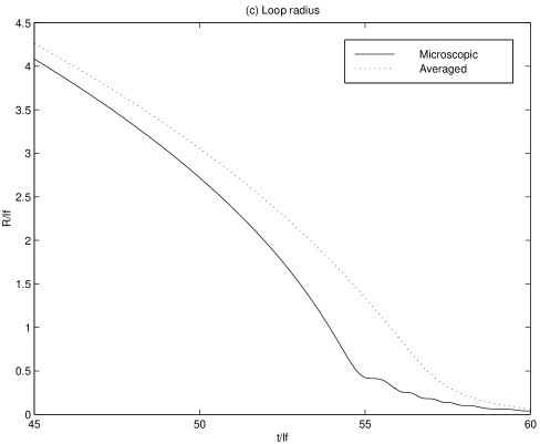
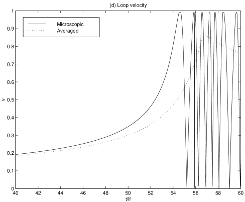
FIG. 3.: Comparing the ‘microscopic’ (solid lines) and ‘averaged’ (dashed) evolution equations for a circular loop in a condensed-matter context. Length and time are in units of $\ell_{\rm f}$, and the time axis is with a linear scale. Plot (a) depicts the log of the (rescaled) radius, while (b) depicts the loop velocity (in units of $c$). The lower graphs are close-ups of the upper ones.

         

         

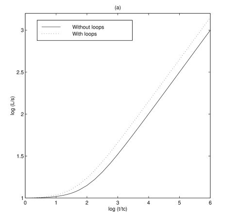
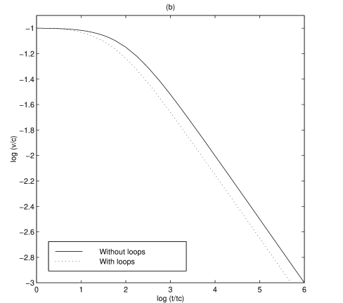
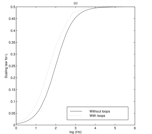
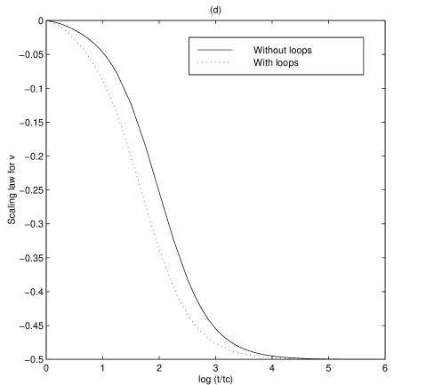
FIG. 4.: The approach to scaling of a network of gauge strings at constant temperature for ${\tilde{c}}=0$ (solid lines) and ${\tilde{c}}=1$ (dotted lines); $k=1$ and the initial conditions are $0.1L_{i}=ct_{i}=s$, $v_{i}=0.1\,c$. The plots correspond to the evolution of $L/s$ (a) and $v$ (in units of $c$) (b) and the exponents of the power-law dependence of $L$ (c) and $v$ (d). The horizontal axis is labeled in orders of magnitude in time form the moment of string formation; in (a) an (b), the ‘y’ axis is also in a logarithmic scale.

         

         

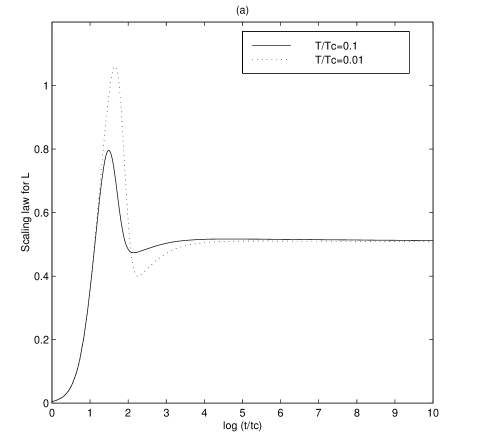
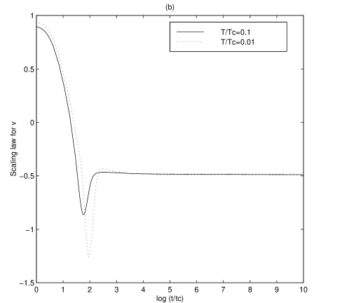
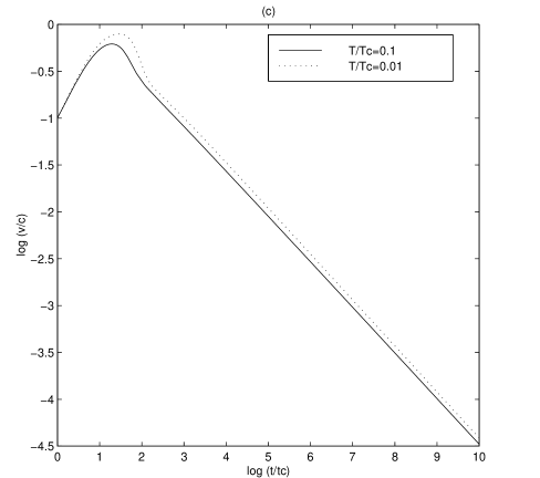
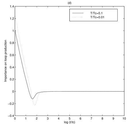
FIG. 5.: The approach to scaling of a network of global strings at constant temperature for $T/T_{c}=0.1$ (solid lines) and $T/T_{c}=0.01$ (dotted lines); ${\tilde{c}}=1$, $k=1$ and the initial conditions are $0.1L_{i}=ct_{i}=s$, $v_{i}=0.1\,c$. The plots correspond to the evolution of the exponents of the power-law dependence of $L$ (a) and $v$ (b), $v$ itself (in units of $c$) (c) and the ratio of the loop formation and friction terms (d). The horizontal axis is labeled in orders of magnitude in time from the moment of string formation; in (c) an (d), the ‘y’ axis is also in a logarithmic scale.

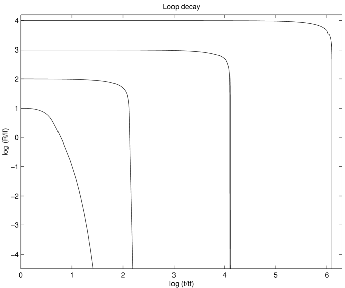
FIG. 6.: The evolution of loops of different sizes relative to the friction lengthscale. For large enough loops, the lifetime is proportional to the square of the length.

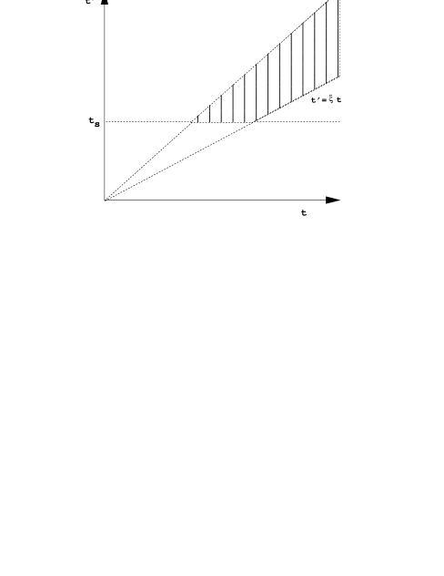
FIG. 7.: The interval in t’ giving a non-zero loop length contribution to the integral (55) for different times t.

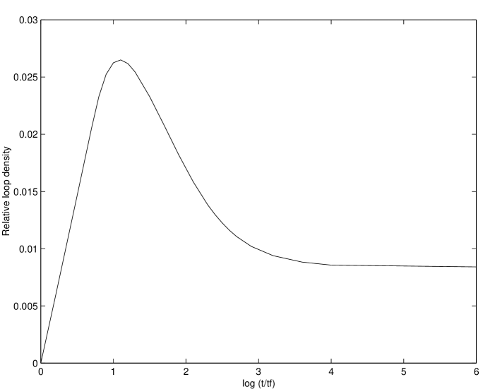
FIG. 8.: The ratio of the loop and long string densities for a network of gauge strings with ${\tilde{c}}=1$. Initial conditions are as in the corresponding case of figure 4

         

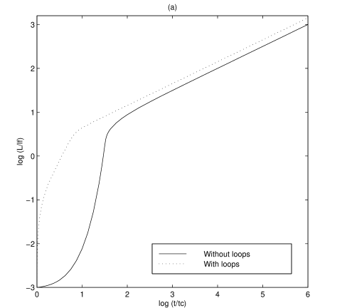
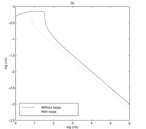
FIG. 9.: The evolution of an initially free network at constant temperature, for ${\tilde{c}}=0$ (solid lines) and ${\tilde{c}}=1$ (dotted lines). Plots represent the lengthscale relative to the friction length (a), velocity (in units of $c$) (b) and ratio of long-string and loop energy densities (c); all are log-log plots (time is in orders of magnitude after the network formation). Notice that the exponential growth in $L$ (aided by the relativistic velocity) leads to a period of loop domination.

- [1] D. Mermin, Rev. Mod. Phys. 51, 591 (1979).
- [2] I. Chuang et al., Science 251, 1336 (1991).
- [3] P. de Gennes, ‘The physics of liquid crystals’, Clarendon Press, Oxford (1981); M. Bowick et al., Science 263, 947 (1994).
- [4] M. Salomaa and G. Volovik, Rev. Mod. Phys. 59, 533 (1987); U. Parts et al., Phys. Rev. Lett. 75, 3320 (1995).
- [5] W. H. Zurek, Nature 317, 505 (1985); P C. Hendry et al., Nature 368, 315 (1994).
- [6] A. Abrikosov, Sov. Phys. JETP 5, 1174 (1957).
- [7] A. Vilenkin and E. P. S. Shellard, ‘Cosmic Strings and other Topological Defects’, Cambridge University Press (1994).
- [8] T. W. B. Kibble, J. Mod. Phys. A9, 1387 (1976).
- [9] M. Hindmarsh, A.-C. Davis and R. H. Brandenberger, Phys. Rev. D49, 1944 (1994); R. H. Brandenberger and A.-C. Davis, Phys. Lett. B332, 305 (1994).
- [10] T. W. B. Kibble, Nucl. Phys. B252, 227 (1985); B261, 750 (1986).
- [11] D. Austin, E. J. Copeland and T. W. B. Kibble, Phys. Rev. D48, 5594 (1993).
- [12] A. J. Bray, Adv. Phys. 43, 357 (1994), and references therein.
- [13] D. P. Bennett, Phys. Rev. D33, 872 (1986); Phys. Rev. D34, 3592 (1986).
- [14] A. Albrecht and N. Turok, Phys. Rev. D40, 973 (1989).
- [15] C. J. A. P. Martins and E. P. S. Shellard, Phys. Rev. D53, 575 (1996).
- [16] C. J. A. P. Martins and E. P. S. Shellard, Phys. Rev. D54, 2535 (1996).
- [17] A. Vilenkin, Phys. Rev. D43, 1060 (1991).
- [18] R. Rohm, Ph.D. thesis, Princeton University (1985); P. de Sousa Gerbert and R. Jackiw, Comm. Math. Phys. 124, 229 (1988); M. G. Alford and F. Wilczek, Phys. Rev. Lett. 62, 1071 (1989).
- [19] A. E. Everett, Phys. Rev. D24, 858 (1981); W. B. Perkins et al., Nucl. Phys. B353, 237 (1991).
- [20] K. W. Schwarz, Phys. Rev. B38, 2398 (1988).
- [21] R. L. Davis and E. P. S. Shellard, Phys. Rev. Lett. 63, 2021 (1989).
- [22] J. Garriga and M. Sakellariadou, Phys. Rev. D48, 2052 (1993).
- [23] I. M. Lifshitz, Zh. Eksp. Teor. Fiz. 42, 1354 (1962); S. M. Allen & J. W. Cahn, Acta Metall. 27, 1085 (1979).
- [24] R. E. Blundell and A. J. Bray, Phys. Rev. E49, 4925 (1994); M Mondello and N. Goldenfeld, Phys. Rev. A45, 657 (1992); H. Toyoki, J. Phys. Soc. Jpn. 60, 1433 (1991).
- [25] A. J. Bray and A. D. Rutenberg, Phys. Rev. E49, R27 (1994).