Griffiths singularities in the two dimensional diluted Ising model

Abstract

We study numerically the probability distribution of the Yang-Lee zeroes inside the Griffiths phase for the two dimensional site diluted Ising model and we check that the shape of this distribution is that predicted in previous analytical works. By studying the finite size scaling of the averaged smallest zero at the phase transition we extract, for two values of the dilution, the anomalous dimension, $\eta$, which agrees very well with the previous estimated values.

1 Introduction

The Yang-Lee theorem provides a theoretical, and powerful, tool to study phase transitions. In systems without disorder (e.g. the usual $\phi^{4}$ theories or Ising models, XY model, etc) this theorem allows to characterize and to estimate numerically the phase transition and the anomalous dimension [1, 2].

In the disordered case (i.e. systems with a random interactions) the theorem provides a tool to study (and to define) the Griffiths phase (or in other words the Griffiths singularities) [3]. The Griffiths phase is a peculiar phenomenon of disordered systems. Roughly, it is a region above the critical temperature of the disordered system and below that of the pure system (for some choices of the disorder distribution this temperature could be infinite [4]). Below the critical temperature of the pure system, which we denote $T_{c}(p=1)$, but above the critical temperature of the disordered one, which we denote $T_{c}(p)$, there exist magnetized domains (geometrical clusters, since of course, the total magnetization is zero, as we are still in the paramagnetic phase of the diluted system). These domains of non-zero magnetization induce a complex singularity (Yang-Lee zeroes) in the free energy as a function of the magnetic field (Griffiths singularity [3]).

In classical statistical mechanics the Griffiths singularities are essential singularities and so have no effect on the static properties of the system (nothing diverges in the Griffiths phase, except at the critical point).

But dynamically this phase induces a slow behavior in the spin-spin autocorrelation functions [6] , the dynamic of the system becomes slower than in the “usual” paramagnetic phase [4].

For instance, in the three dimensional spin glass case, numerically there is a change in the autocorrelations functions from those of the paramagnetic case ($C(t)\sim t^{-x}\exp(-at)$) to a short range correlations (like a behavior : $C(t)\sim t^{-x}\exp(-at^{\beta}),\;\;\beta\neq 1$ ) just at the critical point of the pure Ising model. Obviously at the critical point of the $3d$ spin glass there exists another change in the behavior of the autocorrelation function to a spin glass regime [6].

In this paper we will focus our attention on the probability distribution of the smallest zero in the Griffiths phase and we will confront our numerical results with the analytical prediction of reference [4]. We have obtained a clear numerical picture about the construction of the Griffiths singularities.

We will also extract, using the scaling of the average of the smallest zeroes at the critical point, the anomalous dimension of the system and we will compare this value with previous numerical simulations of the system [8].

2 Yang-Lee singularities

By regarding the partition function of the pure Ising model in a finite volume $L^{d}$ as a function of the variables

$$\rho=e^{-2h}\;\;,\;\;\;\tau=e^{-2\beta},$$

where $h$ is the magnetic field and $\beta$ is the inverse of the temperature, Yang and Lee [9, 10] found that the complex zeroes of the partition function in the $\rho$ variable lie in the unit circle and there are no zeroes on the real axis. Moreover in the thermodynamical limit, and for $\beta\geq\beta_{c}$, the point $\rho=1$ becomes an accumulation point giving rise to a singularity in the free energy.

Near the critical point, in the paramagnetic phase, the imaginary part of the zero nearest to the real axis, $h_{s}$, behaves

$$h_{s}\sim(\beta_{c}-\beta)^{\Delta},$$ (1)

and then, in the standard way, we can write down the finite–size dependence of $h_{s}$ at the critical point

$$h_{s}\sim L^{-(\Delta/\nu)}.$$ (2)

Using the scaling relation $\Delta=\nu d-\beta$, where $d$ is the dimension, we can rewrite the last equation as

$$h_{s}\sim L^{-(2-\eta/2)}.$$ (3)

Below the phase transition, in the ferromagnetic phase, the scaling law is

$$h_{s}\sim L^{-d}.$$ (4)

In the disordered case, each sample will have a smallest $h$, that we hereafter denote as $h_{\epsilon}$. We will investigate numerically the functional form of the probability distribution of $h_{\epsilon}$, that we will write as $p(h_{\epsilon})$.

There are some analytical results about the density of the zeroes in the Griffiths phase. The authors of reference [4] obtain for the density of zeroes, with imaginary part $h_{i}$, of a diluted Ising system with a proportion of spins $p$ the following law

$$\rho(h_{i})\propto\exp(\frac{A\log(p)}{h_{i}}),$$ (5)

as $h_{i}\ll 1$, which is a very weak dependence.

It has been assumed that a cluster of size $L$ introduces a zero, which induces the previous law, that scales as (see equation (4))

$$h_{i}=\frac{A}{L^{d}}.$$ (6)

where $A$ is the inverse of the site magnetization of the cluster [4].

It is possible to obtain a better estimate of the prefactor of $1/h_{i}$ in the exponential of the formula (5) using a variational method [4].

The important point is that there is a finite probability to have a zero in any neighborhood of $h=0$.

To complete this discussion we will add that at the critical point the density arrives with a non zero slope to the origin, in the broken phase the density at the origin is finite, and above of the critical temperature of the pure system the density is zero in a neighborhood of the origin [4].

3 The model and the numerical method

The simplest disordered system is the diluted Ising model. This model describes, for instance, the Anderson localization [11], and has been studied analytically (using the mapping to a O($N$) theory with cubic anisotropy in the limit $N\rightarrow 0$) [11, 12] and numerically [13, 17, 14, 8].

The Hamiltonian of the two dimensional site diluted Ising model in a hypercubic lattice of size $L$ with periodic boundary conditions is

$${\cal H}_{\epsilon}=-\sum_{<ij>}\epsilon_{i}\epsilon_{j}\sigma_{i}\sigma_{j},$$ (7)

where $<ij>$ denotes nearest neighbors pairs, $\sigma_{i}$ are the usual spin variables and $\epsilon_{i}$ are independent quenched noises which are $1$ with probability $p$ and $0$ with probability $1-p$. Obviously the system will have a phase transition only if $p\geq p_{c}$ where $p_{c}$ is the percolation threshold for the $d$-dimensional site percolation. For instance, in two dimension $p_{c}=0.592746$ [15].

There are analytical results for this model mainly by Dotsenko and Dotsenko, and Shalaev [16] (DDS) using Renormalization Group techniques. There is a change in the functional form of the specific heat (from $\log|t|$ to $\log[1+a\log|t|]$, where $|t|$ is the reduced critical temperature and $a$ is a constant), but there is no change in the $\nu$ exponent. This result must hold for a lower dilution of spins. For this weak disorder there are numerical results that support this picture [17].

But the authors of reference [8] claim that the specific heat follows the prediction of (DDS) but only for a lower degree of dilution, moreover they found a dependence of the $\nu$ and $\gamma$ exponents with the dilution such that the $\eta$ exponent is constant (we remark that $\gamma/\nu=2-\eta$).

The end-point of the critical line (in the plane $(\beta,p)$), $(\beta=\infty,p_{c})$, has critical exponents $\nu=4/3$ and $\gamma=43/18$ which implies $\eta=5/24\approx 0.2083$ [15].

The partition function for a purely imaginary magnetic field, $ih$, in a $d$-dimensional lattice of size $L$ is

$${\cal Z}(\beta,h)=\sum_{[\sigma]}\exp(\beta\sum_{<ij>}\sigma_{i}\sigma_{j}+ih\sum_{i}\sigma_{i}).$$ (8)

By defining $M=\sum_{i}\sigma_{i}$, the total magnetization of the system, we obtain

$${\cal Z}(\beta,h)=\langle\cos(hM)\rangle+i\langle\sin(hM)\rangle,$$ (9)

where the average $\langle(\cdot\cdot)\rangle$ is taken with ${\cal Z}(\beta,h=0)$, i.e. a real measure. In the paramagnetic phase all the odd moments of the magnetization vanish, which implies $\langle\sin(hM)\rangle=0$ and the only singularities of the free energy ($\log{\cal Z}(\beta,h)$) will arise from the zeroes of $\langle\cos(hM)\rangle$.

This is the scenario for the pure systems. In the diluted case we need to replace $\sigma_{i}$ by $\epsilon_{i}\sigma_{i}$ and so each samples will have its own smallest zero ($h_{\epsilon}$). The averaged values over all the samples, ${\overline{h_{\epsilon}}}$, should follow the previous finite–size scaling relation (3) at criticality.

4 Probability distribution of the Yang-Lee zeroes in the Griffiths phase

To check the analytical form of the probability distribution, $p(h_{\epsilon})$, of the smallest Yang-Lee zeroes we have done numerical simulations with $\beta=0.52$ and $p=0.889$ which is inside of the Griffiths phase. We used the Wolff algorithm [19] and we simulated the sizes $L=4$ (8000 samples), $L=8$ (15000 samples), $L=12$ (2200 samples) and $L=16$ (3926 samples). The results are shown in Figure 1.

Figure 1: Probability distribution of the smallest zeroes for (right to left) $L=8$, $L=12$ and $L=16$.

We expect that the minimum value of $h_{\epsilon}$, at fixed $L$, should be due to the sample with all the points filled (i.e. a pure Ising model of size $L$). We find that the minimum smallest zero, as a function of the lattice size, follow the rule

$$h_{\epsilon}^{\rm min}=\frac{1.5(1)}{L^{1.93(4)}},$$ (10)

where we have fitted using $4\leq L\leq 12$ with $\chi^{2}/{\rm DF}=0.2/1$ (DF means degrees of freedom).

For $L\geq 16$ lattices the previous fit (10) does not hold. This discrepancy comes from the fact that the number of samples that we need to pick up this minimum value is larger than the number that we have simulated.

Simulating directly the pure Ising model we find that the smallest zero (simulating up to $L=32$), as a function of the sizes, at $\beta=0.52$ (ordered phase of the pure model) behaves

$$h^{\rm min}_{\rm pure}=\frac{1.55(4)}{L^{1.97(1)}},$$ (11)

following very well the law (4). The agreement with eq. (10) is also very good.

We have also fitted the mean value of the probability distribution as a function of $L$ (for $L$=$8$, $12$, $16$, $64$, $128$, $192$) in the diluted case and we have found that the numerical data behave

$$\overline{h_{\epsilon}}=0.0041(1)+1.67(2)L^{-1.84(1)},$$

with a very good $\chi^{2}/{\rm DF}=4.9/4$. The samples used for $L\geq 64$ are written in Table 1.

We plot in Figure 2 the head (i.e. the region of lower values of $h$) of the probability distribution for the $L=8$ lattice in the variables $(1/h_{\epsilon},\log p(h_{\epsilon}))$ in order to check the formula (5).

We see two different regions that we mark with two linear fits. The first region (left part of the figure) has a slope ($-0.11(3)$) which agrees, is a two standard deviation, with the naive theoretical prediction ($(\log p)A=(1.5(1)\times\log\frac{8}{9})=-0.18(1)$), where we have used for $A$ the numerator of the fit (10). The second region decays with a behavior compatible with the equation (5) but the slope is wrong (slope= $-0.94(4)$). We think that this decay is due to a finite–size effect (the lattice size is 8) and hides the decay with the “naive” slope ($\approx-0.18$).

Bray [4] shows that the real slope (in absolute value) has as upper bound the “naive value” (0.18). Our numerical results go in this direction. In particular as $T\rightarrow T_{c}(p)^{+}$ the real slope, in absolute value, goes to zero however the “naive” value will clearly be different from zero.

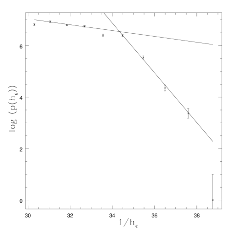
Figure 2: Head of the logarithm of the probability distribution (modulo a normalization factor) of the smallest zeroes for $L=8$ as a function of $1/h_{\epsilon}$.

Hence, the numerical picture is as follows (we remark that we are in the Griffiths phase): we have a narrow probability distribution with its mean value having a non zero thermodynamic limit. But the minimum value of this probability distribution follows the law of the pure Ising model in the ferromagnetic phase so that goes to zero and introduces a singularity in the free energy. We have seen this behavior when simulating a large number of samples up to $L=12$. Using a very large number of samples could be possible to continue this result to large lattices ($L\geq 16$).

We will see in the next section how, at the critical point, the mean value of the smallest zeroes goes to zero following a power law.

5 Scaling of the Yang-Lee zeroes at $T_{c}$

At $T_{c}$ we have performed numerical simulations using the Wolff algorithm with two degree of dilution, $p=0.889$ and $p=0.75$, and lattice sizes $L=64,128,192$ and $256$. We report in Table 1 the number of samples used.

$L$	$p=0.889$	$p=0.75$
64	100	100
128	40	40
196	30	40
256	30	40

Table 1: Number of samples simulated for different sizes and dilutions used in the numerical simulations of sections 4 and 5.

We have used the values of the inverse critical temperatures ($\beta_{c}(p)$) reported in reference [8] . We will also compare the results of this reference with our result for the $\eta$ exponent.

$p$	$\gamma/\nu$	$\eta$	$\gamma/\nu$	$\Delta/\nu$	$\eta$
0.889	1.72(1)	0.279(14)	1.75(2)	1.873(13)	0.254(26)
0.75	1.72(3)	0.28(3)	1.76(3)	1.89(2)	0.22(4)

Table 2: Results for the critical exponents. The first column is the proportion of spins. The next two columns are the critical exponents reported in reference [8]. The fourth and fifth ones are our estimates of $\gamma/\nu$ (as control, calculated as $\chi_{\rm max}\approx L^{\gamma/\nu}$) and $\Delta/\nu$ (using the scaling of the zeroes) respectively. In the last column we report $\eta$ calculated using the scaling relation $\eta\equiv 4-2\Delta/\nu$.

We have measured the susceptibility,

$$\chi=\frac{1}{V}\overline{\langle M^{2}\rangle},$$

where $\overline{(\cdot\cdot)}$ is the average on the disorder and $\langle(\cdot\cdot)\rangle$ is the thermal average. We have also measured $\langle\cos(hM)\rangle$ in every sample to calculate the zeroes.

We obtain $h_{\epsilon}$, the smallest zero for each sample, and then we calcule the mean value, ${\overline{h}_{\epsilon}}$. The error is estimated using sample to sample fluctuations. We plot the finite–size scaling in Figure 3 and Figure 4, for $p=0.889$ and $p=0.75$ respectively, with our best power fits drawn as a line (fifth column of Table 2). We report the numerical values of the fit (also for the susceptibility) in Table 2. The second and third columns of the Table 2, are the estimates of reference [8] for $\gamma/\nu$ and $\eta$, obtained as $2-\gamma/\nu$.

Figure 3: Mean value of the smallest Yang-Lee zeroes,$<h_{\epsilon}>\equiv\overline{h}_{\epsilon}$, against the size, in a double logarithmic scale for a dilution $p=0.889$. The straight line is the power law fit reported in Table 2 and text. This fit has a $\chi^{2}/{\rm DF}=0.11$.

Table 2 shows that our values of $\gamma/\nu$ are in the errors with those of reference [8] (we perform this as check) and this also holds with our estimate of $\eta$ using scaling of zeroes. The results are compatibles with $\eta=0.25$ on the critical line.

Figure 4: Mean value of the smallest Yang-Lee zeroes against the size in a double logarithmic scale for a dilution $p=0.75$. The straight line is the power law fit reported in Table 2 and text. This fit has a $\chi^{2}/{\rm DF}=0.28$.

6 Conclusions

We have investigated the Griffiths phase by studying the behavior of the probability distribution of the smallest Yang-Lee zeroes. We have obtained a clear numerical picture of the finite–size construction of these singularities. We have also confronted our numerical data with previous analytical results [4] and the agreement is very good.

In the second part of this paper we have shown that the study of the smallest zeroes is very useful to estimate accurately the anomalous dimension of the system.

We have extracted one critical exponent of the system, $\eta$, which agrees with the analytical predictions and with the numerical results. We need to calculate the second one in order to fix the universality class of the Hamiltonian. A possible calculation, in the line to seek complex singularities, is the study of the Fisher zeroes [18]. This study will point out the thermal critical exponent $\nu$ [20] and clarify if it depends on the proportion of spins or not.

References

- [1] R. B. Kenna and C. B. Lang, Phys. Lett. B264 (1991)396.
- [2] R. Kenna and A.C. Irving. hep-lat/9601029.
- [3] R. B. Griffiths, Phys. Rev. Lett. 23 (1969) 17.
-
[4]
A. J. Bray and D. Huifang,
Phys. Rev. B. 40 (1989)6980.
A. J. Bray and M.A. Moore, J. Phys. C: Solid State Phys. 15 (1982) L765-L771.
A. J. Bray, Phys. Rev. Lett. 59 (1987) 586. - [5] H. Rieger and A. P. Young, cond-mat/9512162.
- [6] A. T. Ogielsky, Phys. Rev. B 12 (1985)7384
- [7] F. Cesi, C. Maes and F. Martinelli, Roma-1-1151/96 preprint.
- [8] J-K. Kim and A. Patrascioiu, Phys. Rev. Lett. 72 (1994) 2785.
- [9] C. N. Yang and T. D. Lee, Phys. Rev 87 (1952) 404.
- [10] C. Itzykson and J-M. Drouffe, Statistical Field Theory, Vol 1, Cambridge University Press 1989.
- [11] G. Parisi, Field Theory, Disorder and Simulations. World Scientific 1994.
- [12] J. L. Cardy and A. J. McKane, Nucl. Phys. B257 FS14 (1985) 383
- [13] G. Parisi and J.J. Ruiz-Lorenzo. J. Phys. A: Math and Gen. 28 (1995)L395.
- [14] J-K. Kim, cond-mat/9502053.
- [15] D. Stauffer and A. Aharony. An introduction to the percolation theory. Revised second edition. Taylor & Francis 1994.
-
[16]
Vi. S. Dotsenko and Vl. S. Dotsenko,
Adv. in Phys. 32, 1219 (1983),
B. N. Shalaev, Sov. Phys. Solid State, 26 (1984) 1811. - [17] H.-O. Heuer, Europhys. Lett., 16(5) 503(1991).
- [18] E. Marinari, Nucl. Phys. B235 (FS11) (1984) 123.
- [19] U. Wolff, Phys. Lett. B 228, 3 (1989).
- [20] J.J.Ruiz-Lorenzo. Work in progress.