Front localization in a ballistic annihilation model.

Abstract

We study the possibility of localization of the front present in a one-dimensional ballistically-controlled annihilation model in which the two annihilating species are initially spatially separated. We construct two different classes of initial conditions, for which the front remains localized.

UGVA-DPT 1996/07-934

1 Introduction

During the last decade, a large body of work has been devoted to the study of the kinetics of diffusion-annihilation processes. It is now well established that, below some upper critical dimension, the fluctuations play a central role and that accordingly mean-field like approximations are inappropriate.

Moreover, for the two species case $A+B\to 0$, when the two reactants are initially spatially separated, a reaction-diffusion front, getting larger with time, is formed [1, 2]. In the long time regime, the time dependent properties of this front (position, width) are characterized by power laws which are non-mean-field at or below two dimensions.

Instead of investigating a time dependent problem, it was shown by Cornell and Droz [3] that it may be advantageous to study the front formed in the steady state reached by imposing antiparallel currents $J_{A}=|J|$ and $J_{B}=-|J|$ of A- and B-particles at $x=-\infty$ and $x=+\infty$ respectively. It turns out that first, exact prediction can be made in the one dimensional case and second this stationary problem is closely related to the time-dependent one.

More recently, a different but related problem has been considered, namely the case of ballistically-controlled annihilation processes. Most of the results obtained are for the one dimensional case. Initially, the particles are randomly distributed in space and their velocities are distributed according to a given distribution. The particles move freely and when two of them collide they instantaneously annihilate each other and disappear out of the system [4, 5, 6, 7, 8, 12]. In 1985, Elskens and Frisch [4] considered the case of one species of particles moving with velocities $+c$ and $-c$. The case of an arbitrary discrete velocity distribution has been studied by Droz, Rey, Frachebourg and Piasecki [7, 8] and exactly solved for a symmetric three velocities distribution, using an exact closure of the hierarchy obtained previously by Piasecki [6]. Such processes can model several physical situations as a recombination reaction in the gas phase or the fluorescence of laser excited gas atoms with quenching on contact (the one-dimensional aspect can be obtained by working in a suitable porous media [9]) or, the annihilation of kink-antikink pairs in solid state physics [10].

We have recently investigated the case of the front formation for ballistic annihilation with two species initially separated in space in one-dimension [12]. This process can model, for example, the situation in which chemical species incorporated in a gel move ballistically under the action of a drift [11]. As the two species cannot penetrate one into the other (as they annihilate on contact), a well defined reaction front is formed. For a symmetrical Poissonian-type initial spatial distribution, we have proved [12] that the front behaves like a random walker for long time. In other words, at long time, the front can be anywhere on the line: it is delocalized.

In view of what has been done for the diffusive case, it is natural to try to find a system with ballistic-annihilation possessing a localized reaction front. Let us first remark that in the ballistic case, to impose a flux of particles at the boundaries of a finite system is equivalent to fix an initial spatial distribution of a large system. For example, the case with homogeneous spatial Poisson distribution can be mapped onto a system with boundary fluxes of particles at constant rate, the time between two particles input being exponentially distributed.

Thus we shall consider the problem in terms of initial distribution of particles and ask the question: is it possible to localize the front by choosing a suitable initial distribution of the particles ? The answer is obviously yes. Indeed, as a simple example, consider the case in which initially each particle is located on a regular lattice, the $A$ particles being to the left of the origin and the $B$’s to the right, in a symmetric way. The position at which collision between one $A$ and one $B$ particle takes place defines the position of the annihilation front. Thus the front will always sit at the origin. However, this case is pathological in the sense that the initial state is totaly ordered. For more general situations, with spatial randomness in the initial state, we have first to define what is meant by ”localisation of the front”. Then we shall show that indeed, it is possible to find suitable initial conditions localizing the front.

The paper is organized as follows. In section 2, we define precisely the class of models studied and introduce several criterions of localisation. In section 3, we consider a class of correlated initial conditions for which we are able to compute the probability density $\mu(X;t)$ to find the front at position $X$ at time $t$ and which leads to the localization of the front. In section four, we consider a different class of initial conditions with no correlations between the initial positions of particles. For this more physical class of initial conditions, we are not able to compute explicitly $\mu(X;t)$, but we can show that the mean square position of the front $\langle X^{2}\rangle$ converges for $t\to\infty$. This means that the probability density $\mu(X;t)$ does not spread out. Remarks and conclusions are drawn in section 5.

2 The model and the criterion of localization.

We consider a one-dimensional system formed of two species of particles. Initially, particles $A$ are spatially randomly distributed in the region $(-\infty,0)$ and the $B$ ones are spatially randomly distributed in the region $(0,\infty)$. For the sake of simplicity we shall consider only symmetric distributions in $A$ and $B$. In particular, $\rho_{A}(-x)=\rho_{B}(x)=\rho(x),x>0$, where $\rho_{A}$ and $\rho_{B}$ are the number densities of particles $A$ and $B$ respectively. For nonsymmetric distributions, the front moves acquiring some mean velocity.

The velocity of each particle is an independent random variable taking the value $\pm c$ with equal probability. Particles of the same kind suffer elastic collisions. When two particles $A$ and $B$ meet, they annihilate. Thus, practically the $A$ particles with velocity $-c$ and the $B$ particles with velocity $+c$ move freely. Accordingly, the relevant part of the dynamics concerns only the $A$ particles with velocity $+c$ and the $B$ ones with velocity $-c$.

Let $(y_{1},y_{2},\ldots,y_{k},\ldots)$ be the initial positions of the $A$ particles with velocity $+c$ and $(x_{1},x_{2},\ldots,x_{k},\ldots)$ the initial positions of the $B$’s with velocity $-c$. The particles are labeled such that $y_{k}<\cdots<y_{1}<0<x_{1}<\cdots<x_{k}$. The relative velocity between the $A$ and $B$ particles being $2c$, the pair of particles initially at $(x_{k},y_{k})$ will collide at time $t_{k}=(x_{k}-y_{k})/2c$. The position at which this collision will take place defines the position of the annihilation front. Thus, the position of the front at time $t$ is $(x_{1}-y_{1})/2c$, if $2ct\leq x_{1}+y_{1}$ (i.e. if no particle has yet collided), $(x_{2}-y_{2})/2c$, if $x_{1}+y_{1}\leq 2ct\leq x_{2}+y_{2}$ (i.e. only the first particles on the right and on the left have collided), and so on. The dynamics in itself is purely deterministic, the only stochastic aspect comes from the initial conditions.

The properties of the front are completely defined by the probability density $\mu(X;t)$ to find the front at the point $X$, at time $t$. In a previous paper [12], we have proved that:

$$\mu(X;t)=\left\langle\delta(X-{\textstyle\frac{1}{2}}[x_{1}+y_{1}])\right\rangle$$

$$+ \left\langle\sum_{k=1}^{\infty}\left[\delta(X-{\textstyle\frac{1}{2}}[x_{k+1}+y_{k+1}])-\delta(X-{\textstyle\frac{1}{2}}[x_{k}+y_{k}])\right]\theta(2ct-[x_{k}-y_{k}])\right\rangle\,,$$

where $\delta$ and $\theta$ are the usual Dirac and Heaviside functions and the brackets denote the average over the initial positions, according to the initial distribution. It follows that, the second moment of $\mu(X;t)$ is

$$\langle X^{2}\rangle = \left\langle\left(\frac{x_{1}+y_{1}}{2}\right)^{2}\right\rangle$$ (2)

$$+ \sum_{k=1}^{\infty}\left\langle\left[\left(\frac{x_{k+1}+y_{k+1}}{2}\right)^{2}-\left(\frac{x_{k}+y_{k}}{2}\right)^{2}\right]\theta\left(2ct-[x_{k}-y_{k}]\right)\right\rangle\,.$$

Several criterions can be introduced to define the localization of the front. The first is simply to ask that $\mu(X;t)$ approches for $t\to\infty$ a limiting distribution with finite moments. A second criterion consists in asking that $\mu(X;t)$ has a compact support with respect to $X$, for all time. These two criterions are useful provided that one is able to compute $\mu(X;t)$. This calculation will be possible for our first class of initial conditions (section 3).

However to deal with the second class of initial conditions, we are led to propose a weaker definition of the localization. The front will be said to be localized if $\mu(X;t)$ has a finite second moment (or variance in case of a non-symmetric initial distribution) for all time $t\leq\infty$.

We know what is happening in two limit cases. For a Poisson distribution the front is not localized while for particles regularly distributed on a lattice the front is strongly localized. It is thus natural to consider an initial distribution which extarpolates smoothly between these two limits. Such distribution is provided by the Erlang-k-process [13]. For $k=1$, one recovers the Poisson process while for $k\to\infty$ one finds the case of the regular distribution. However, it can be shown [14] that for all finite values of $k$ the front is delocalized. Only the limit case $k\to\infty$ is localized.

3 Correlated initial distribution.

We aim at finding a class of initial conditions for which the probability density $\mu(X;t)$ has a compact support, with respect to X. This property can be obtained with the following initial condition: each $B$ particle is uniformly distributed in an interval of length $\delta<\ell$, centered at $(k-{\textstyle\frac{1}{2}})\ell$, where $\ell$ is the distance (center-to-center) between two consecutive intervals and $k$ labels the particles $(k=1,2,\dots)$. We use the same distribution for particles $A$, but on the left of the origin. First, remark that the position of any particle is completely independent of the other; in addition we choose identical distribution for each particles, but at different regularly spaced positions. We eventually conclude that $\mu(X;t)$ must be a time periodic function of period $\ell/c$. Hence it is enough to compute $\mu(X;t)$ for $t\in[0,\ell/c)$. In this case, eq. (2) simply reduces to

$$\mu(X;t) \equiv \nu_{0}(X)+\nu(X;t)$$

$$= \left\langle\delta(X-{\textstyle\frac{1}{2}}[x_{1}+y_{1}])\right\rangle$$

$$+ \left\langle\left[\delta(X-{\textstyle\frac{1}{2}}[x_{2}+y_{2}])-\delta(X-{\textstyle\frac{1}{2}}[x_{1}+y_{1}])\right]\theta(2ct-[x_{1}-y_{1}])\right\rangle\,.$$

The first bracket reads

$$\nu_{0}(X) = \frac{1}{\delta^{2}}\int_{-\frac{\ell+\delta}{2}}^{-\frac{\ell-\delta}{2}}{\d}y_{1}\int_{\frac{\ell-\delta}{2}}^{\frac{\ell+\delta}{2}}{\d}x_{1}\,\delta(X-{\textstyle\frac{1}{2}}[x_{1}+y_{1}])$$ (4)

$$= \frac{4}{\delta^{2}}\left(\frac{\delta}{2}-|X|\right)\theta({\textstyle\frac{1}{2}}\delta-|X|)\,.$$

The computation of the second bracket is less straightforward, mainly due to the presence of the Heaviside function:

$$\nu(X;t) = \frac{1}{\delta^{4}}\int_{-\frac{3\ell+\delta}{2}}^{-\frac{3\ell-\delta}{2}}{\d}y_{2}\int_{\frac{3\ell-\delta}{2}}^{\frac{3\ell+\delta}{2}}{\d}x_{2}\int_{-\frac{\ell+\delta}{2}}^{-\frac{\ell-\delta}{2}}{\d}y_{1}\int_{\frac{\ell-\delta}{2}}^{\frac{\ell+\delta}{2}}{\d}x_{1}\,\theta\left(2ct-[x_{1}-y_{1}]\right)$$ (5)

$$\times \left[\delta(X-{\textstyle\frac{1}{2}}[x_{2}+y_{2}])-\delta(X-{\textstyle\frac{1}{2}}[x_{1}+y_{1}])\right]\,,$$

However, simplifications arise by doing a Laplace-transform. Carrying the four integrations over $y_{1}$, $y_{2}$, $x_{1}$ and $x_{2}$ and inverting, we finally obtain, $\nu(X;t)$ as a product of the Heaviside function $\theta({\textstyle\frac{1}{2}}\delta-|X|)$ and a sum of five terms. We shall not reproduce these terms here as they are a little bit cumbersome. Nonetheless, we plotted both $\mu(X;t)$ and $\nu(X;t)$ for $t\in[0,\ell/c)$ (see figure 1 and 2). The plot of $\nu(X;t)$ shows that it is not a simple function: already at this stage, $\mu(X;t)$ has a non-trivial shape.

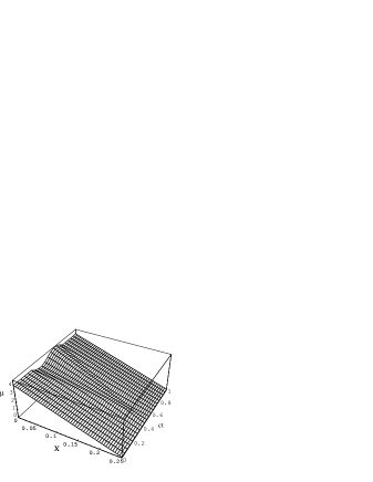
Figure 1: Plot of $\mu(X;t)$, for $\ell={\textstyle\frac{1}{2}}$, $\delta={\textstyle\frac{1}{4}}$, $X\in[0,{\textstyle\frac{1}{4}}]$ and $ct\in[0,1]$. The probability density $\mu(X;t)$ is symmetric with respect to $X$ and periodic (with period $1$) with respect to $ct$.

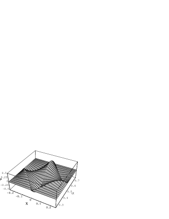
Figure 2: Plot of $\nu(X;t)$, for $\ell={\textstyle\frac{1}{2}}$, $\delta={\textstyle\frac{1}{4}}$, $X\in[-{\textstyle\frac{1}{4}},{\textstyle\frac{1}{4}}]$ and $ct\in[{\textstyle\frac{1}{4}},\frac{3}{4}]$.

It is clear that if we take an arbitrary distribution instead of a uniform one for the probability density inside each interval, we should always find that the support of $\mu(X;t)$ is $[-{\textstyle\frac{1}{2}}\delta,{\textstyle\frac{1}{2}}\delta]$, although the detailed shape of $\mu(X;t)$ may vary considerably. Moreover, one can easily generalize all these statements to non-symmetric distributions, by taking into account that the front will move. The support of $\mu$ will not be the same for all time, as it will follow the mean position of the front.

4 Noncorrelated initial conditions.

In this section we show that the front can be localized by a generalized Poisson-type distribution. For a homogeneous symmetric Poissonian particle distribution, we found [12]:

$$\langle X^{2}\rangle\sim\frac{ct}{2\rho}+\mathrm{Const}\quad(t\to\infty)\,,$$ (6)

where $\rho$ is the initial density. Now suppose that instead of having a constant $\rho$, the density increases with position according to a power law:

$$\rho\equiv\rho(x)=x^{\alpha}\,.$$ (7)

Then, the front (whose average position is the origin) will see an increasing density in time. We can expect to obtain

$$\langle X^{2}\rangle\sim\frac{(ct)^{1-\alpha}}{2}+\mathrm{Const}\quad(t\to\infty)\,.$$ (8)

For $\alpha>1$, $\langle X^{2}\rangle$ converges to a constant, leading to a localization of the front, whereas for $\alpha<1$, it diverges and the front is delocalized. The mechanism leading to the this result is clear: when we increase the density, the mean distance between two successive particles decreases and thus two consecutive collisions should happen relatively often. As a consequence, as the time grows, the probability to find the front far from its mean value becomes smaller. We shall now make more precise this qualitative picture.

To begin we choose, as indicated, the initial particle distribution to be an inhomogeneous Poisson law. In other words, if there is a $B$ particle at position $x_{1}$, the probability to find its right nearest neighbor at position $x_{2}>x_{1}$ is

$$\pi(x_{2},x_{1})=\rho(x_{2})\exp\left[-\int_{x_{1}}^{x_{2}}\rho(z){\d}z\right]\,,$$ (9)

where $\rho(x)$ should be understood as the initial particle density at point $x$. For $\rho(x)=\mathrm{Const}$, we find again the homogeneous Poisson law already studied. The probability to find $k-1$ particles between $0$ and $x_{k}$ and a particle at $x_{k}$ is

$$\pi_{k}(x_{k}) = \rho(x_{k})\int_{0}^{x_{k}}{\d}x_{k-1}\,\exp\left[-\int_{x_{k-1}}^{x_{k}}{\d}z\,\rho(z)\right]$$ (10)

$$\times \rho(x_{k-1})\int_{0}^{x_{k-1}}{\d}x_{k-2}\,\exp\left[-\int_{x_{k-2}}^{x_{k-1}}{\d}z\,\rho(z)\right]\cdots$$

$$\times \rho(x_{2})\int_{0}^{x_{2}}{\d}x_{1}\,\exp\left[-\int_{x_{1}}^{x_{2}}{\d}z\,\rho(z)\right]\rho(x_{1})\exp\left[-\int_{0}^{x_{1}}{\d}z\,\rho(z)\right]$$

$$= \rho(x_{k})\exp\left[-\int_{0}^{x_{k}}{\d}z\,\rho(z)\right]\frac{\left[\int_{0}^{x_{k}}{\d}z\,\rho(z)\right]^{k-1}}{(k-1)!}\,.$$

$\pi_{k}$ is normalized to $1$ provided the density $\rho(x)$ does not vanish at infinity, which is satisfied for the law (7), with $\alpha>0$. The distribution of particles A is chosen in a symmetric way $\rho_{A}(y)=\rho(-y),\,y<0$.

Using eq. (2), the second moment becomes

$$\langle X^{2}\rangle_{t} = \int_{0}^{\infty}{\d}x_{1}\,\rho(x_{1})\exp\left(-\int_{0}^{x_{1}}\rho\right)\int_{-\infty}^{0}{\d}y_{1}\,\rho(y_{1})\exp\left(-\int_{y_{1}}^{0}\rho\right)\left(\frac{x_{1}+y_{1}}{2}\right)^{2}$$ (11)

$$+ \sum_{k=1}^{\infty}\int_{0}^{\infty}{\d}x_{k}\,\rho(x_{k})\int_{-\infty}^{0}{\d}y_{k}\,\rho(y_{k})\int_{x_{k}}^{\infty}{\d}x_{k+1}\,\rho(x_{k+1})\int_{-\infty}^{y_{k}}{\d}y_{k+1}\,\rho(y_{k+1})$$

$$\times \exp\left(-\int_{0}^{x_{k+1}}\rho-\int_{y_{k+1}}^{0}\rho\right)\frac{\left[\int_{0}^{x_{k}}{\d}z\,\rho(z)\right]^{k-1}\left[\int_{y_{k}}^{0}{\d}z\,\rho(z)\right]^{k-1}}{\left[(k-1)!\right]^{2}}$$

$$\times \left[\left(\frac{x_{k+1}+y_{k+1}}{2}\right)^{2}-\left(\frac{x_{k}+y_{k}}{2}\right)^{2}\right]\theta\left(2ct-[x_{k}-y_{k}]\right)\,,$$

where we used the notation

$$\int_{0}^{x_{k}}\rho\equiv\int_{0}^{x_{k}}{\d}z\,\rho(z)\,.$$

Now integrating twice by parts the expression

$$\int_{x_{k}}^{\infty}{\d}x_{k+1}\,\frac{\partial}{\partial x_{k+1}}\left[\exp\left(-\int_{0}^{x_{k+1}}\rho\right)\right]$$

$$\times \int_{-\infty}^{y_{k}}{\d}y_{k+1}\,\frac{\partial}{\partial y_{k+1}}\left[\exp\left(-\int_{y_{k+1}}^{0}\rho\right)\right]\left(\frac{x_{k+1}+y_{k+1}}{2}\right)^{2}$$

and inserting the result into eq. (11), we obtain

$$\langle X^{2}\rangle_{t} = \int_{0}^{\infty}{\d}x\,\rho(x)\int_{0}^{\infty}{\d}y\,\rho(y)\exp\left(-\int_{0}^{x}\rho-\int_{0}^{y}\rho\right)\left(\frac{x+y}{2}\right)^{2}$$ (12)

$$+ \sum_{k=0}^{\infty}\int_{0}^{\infty}{\d}x\,\rho(x)\int_{0}^{\infty}{\d}y\,\rho(y)\frac{\left(\int_{0}^{x}\rho\int_{0}^{y}\rho\right)^{k}}{\left(k!\right)^{2}}$$

$$\times \left[\rule{0.0pt}{19.91692pt}\int_{x}^{\infty}{\d}x^{\prime}\exp\left(-\int_{0}^{x^{\prime}}\rho-\int_{0}^{y}\rho\right)(x^{\prime}-y)\right.$$

$$- \left.\rule{0.0pt}{19.91692pt}{\textstyle\frac{1}{2}}\int_{x}^{\infty}{\d}x^{\prime}\int_{y}^{\infty}{\d}y^{\prime}\exp\left(-\int_{0}^{x^{\prime}}\rho-\int_{0}^{y^{\prime}}\rho\right)\right]\theta\left(2ct-[x+y]\right)\,.$$

We go on by choosing:

$$\rho(x)=x^{\alpha}\,,$$ (13)

with $\alpha\geq 0$. As long as the time is finite, $\langle X^{2}\rangle_{t}$ is finite for any $\alpha$, because the $\alpha=0$ case appears to be an upper bound. However it can grow arbitrarily when $t$ goes to infinity. Can we find $\alpha>0$ such that $\langle X^{2}\rangle_{t}$ is bounded for any time? It is very difficult to calculate exactly $\langle X^{2}\rangle_{t}$. Even when $t$ is large, we have not been able to find its asymptotic expression. Nevertheless we can put $t\to\infty$ in the expression of $\langle X^{2}\rangle_{t}$ and check its convergence. Clearly, as the first term of eq. (12) is time independent, we only have to care of the infinite sum. In addition, when $t\to\infty$, assuming that we can interchange the limit with the sum and the integrals, the restriction on the domain of integration introduced by the Heaviside function is removed. We are thus left to calculate

$$a_{k} \equiv \int_{0}^{\infty}{\d}x\int_{0}^{\infty}{\d}y\,\frac{x^{\alpha}y^{\alpha}}{(k!)^{2}}\left(\frac{x^{\alpha+1}}{\alpha+1}\frac{y^{\alpha+1}}{\alpha+1}\right)^{k}$$ (14)

$$\times \left[\int_{x}^{\infty}{\d}x^{\prime}\,(x^{\prime}-y)\exp\left(-\frac{{x^{\prime}}^{\alpha+1}}{\alpha+1}-\frac{y^{\alpha+1}}{\alpha+1}\right)\right.$$

$$- \left.\frac{1}{2}\int_{x}^{\infty}{\d}x^{\prime}\int_{x}^{\infty}{\d}y^{\prime}\,\exp\left(-\frac{{x^{\prime}}^{\alpha+1}}{\alpha+1}-\frac{{y^{\prime}}^{\alpha+1}}{\alpha+1}\right)\right]$$

and to check the convergence of $\sum_{k=0}^{\infty}a_{k}$.

By changing the variables

$$a=\frac{x^{\alpha+1}}{\alpha+1}\,,\quad b=\frac{y^{\alpha+1}}{\alpha+1}\,,\quad a^{\prime}=\frac{{x^{\prime}}^{\alpha+1}}{\alpha+1}\,,\quad b^{\prime}=\frac{{y^{\prime}}^{\alpha+1}}{\alpha+1}$$

we get

$$a_{k} = \int_{0}^{\infty}{\d}a\int_{0}^{\infty}{\d}b\,\frac{(ab)^{k}}{(k!)^{2}}\left(\rule{0.0pt}{22.76219pt}\int_{a}^{\infty}{\d}a^{\prime}\,[(\alpha+1)a^{\prime}]^{-\frac{\alpha}{\alpha+1}}\e^{-a^{\prime}-b}\right.$$ (15)

$$\times \left\{[(\alpha+1)a^{\prime}]^{-\frac{1}{\alpha+1}}-[(\alpha+1)b]^{-\frac{1}{\alpha+1}}\right\}$$

$$- \left.\rule{0.0pt}{22.76219pt}\frac{1}{2}\int_{a}^{\infty}{\d}a^{\prime}\int_{b}^{\infty}{\d}b^{\prime}\left[(\alpha+1)^{2}a^{\prime}b^{\prime}\right]^{-\frac{\alpha}{\alpha+1}}\e^{-a^{\prime}-b^{\prime}}\right)\,.$$

We finally obtain (by changing the order of integration over $a$ and $a^{\prime}$ and over $b$ and $b^{\prime}$):

$$a_{k} = (\alpha+1)^{\frac{2}{\alpha+1}-1}\left\{\rule{0.0pt}{17.07164pt}\frac{\Gamma\left(\frac{2}{\alpha+1}+k+1\right)}{\Gamma(k+2)}\right.$$ (16)

$$- \left.\rule{0.0pt}{17.07164pt}\left[k+1+\frac{1}{2(\alpha+1)}\right]\frac{\Gamma^{2}\left(\frac{1}{\alpha+1}+k+1\right)}{\Gamma^{2}(k+2)}\right\}\,.$$

To study the convergence of $\sum_{k=0}^{\infty}a_{k}$, we simply have to study the asymptotic behavior of $a_{k}$. We find (see [15])

$$a_{k}=\frac{1}{2}k^{-2+\frac{2}{\alpha+1}}\left[1-\frac{1}{\alpha+1}+\frac{2}{(\alpha+1)^{2}}+{\cal O}(k^{-1})\right]\,,$$

when $k\to\infty$. It is thus evident that the sum converges if and only if $\int_{k=M}^{\infty}{\d}k\,k^{-2+\frac{2}{\alpha+1}}$ does (where $M$ is any integer sufficiently large). This leads us to the previously announced result: $\langle X^{2}\rangle_{t}$ converges if $\alpha>1$, diverges if $\alpha<1$. For $\alpha=1$, one has a logarithmic divergence.

5 Conclusion

We have exhibited two different classes of initial conditions leading to a localization of the reaction front for this ballistic annihilation model. We have shown that the main physical reason for delocalization is a too slow decay of the probability to find two consecutive particles at an arbitrarily large distance. Even an exponential law characterizing the Poisson distribution is not enough.

Several questions remain to be adressed. One natural extension of this work is to know whether or not a faster decay of the probability distribution of the nearest neighbours (for example a Gaussian probability instead of an exponential one) would lead to localization. Indeed, we know that if the interparticle distribution is

$$\pi(x_{2},x_{1})=x_{2}\e^{-{\textstyle\frac{1}{2}}x_{2}^{2}-{\textstyle\frac{1}{2}}x_{1}^{2}}$$

(see eq. (9)), then $\langle X^{2}\rangle_{t}$ diverges logarithmically.

Perhaps, the distribution

$$\pi(x_{2},x_{1})=\e^{-{\textstyle\frac{1}{2}}(x_{2}-x_{1})^{2}}\,,$$

could lead to a front localization. Another possible extension is related to the case of a more general distribution of the velocities. These more difficult problems are under investigation.

References

• [1] L. Gálfi and Z. Rácz, Phys. Rev. A38, 3151 (1988).
• [2] S. Cornell, M. Droz, and B. Chopard, Phys. Rev. A44, 4826 (1991).
• [3] S. Cornell and M. Droz, Phys. Rev. Lett. 70, 3824, (1993)
• [4] Y. Elskens and H. L. Frisch, Phys. Rev. A31, 3812 (1985).
• [5] E. Ben-Naim, S. Redner and F. Leyvraz, Phys. Rev. Lett. 70, 1890 (1993).
• [6] J. Piasecki, Phys. Rev. E51, 5535 (1995).
• [7] M. Droz, P.-A. Rey, L. Frachebourg and J. Piasecki, Phys. Rev. E51, 5541 (1995).
• [8] M. Droz, P.-A. Rey, L. Frachebourg and J. Piasecki, Phys. Rev. Lett. 75, 160 (1995).
• [9] R. Kopelman, Sciences 241, 1620 (1988).
• [10] M. Büttiker and T. Christen, Phys. Rev. Lett. 75, 1895 (1995).
• [11] E. Kárpáti-Smidróczki, A. Büri and M. Zrinyi, Colloid. Polm. Sci. 273, 857 (1995).
• [12] J. Piasecki, P.-A. Rey and M. Droz, To be published in Physica A (1996).
• [13] J. Medhi, “Stochastic Processes”, J. Wiley (N-Y) edt. (1994)
• [14] P.-A. Rey, M. Droz and J. Piasecki, unpublished.
• [15] P. J. Davis, Gamma Function and Related Functions, in Handbook of Mathematical Functions, edited by M. Abramowitz and I. A. Stegun (Dover, New York, 1972).