Electronic Spectral Functions for Quantum Hall Edge States

Abstract

We have evaluated wavevector-dependent electronic spectral functions for integer and fractional quantum Hall edge states using a chiral Luttinger liquid model. The spectral functions have a finite width and a complicated line shape because of the long-range of the Coulomb interaction. We discuss the possibility of probing these line shapes in vertical tunneling experiments.

The quantum-Hall (QH) effect occurs in high mobility two-dimensional electron systems (2DES’s) under the influence of strong perpendicular magnetic fields. Kinetic energy quantization and strong correlations between electrons can lead to discontinuities in the dependence of the chemical potential of the system on density at zero temperature, i.e. to incompressible ground states. Although no gap-less charged excitations of incompressible states can occur in the bulk of the system, the fact that these states occur[1] at magnetic field dependent densities implies that gap-less charged excitations do occur at the edge of the 2DES. The physics of edge excitations has played an important role in explaining transport properties of QH systems[2, 3, 4, 5]. The edge of a 2DES in the QH effect regime is an interesting and in many senses an ideal realization of a one-dimensional (1D) Fermion system[6, 7, 8]. A unique feature is the spatial separation of the left- and right-moving branches of the spectrum which is permitted by time-reversal symmetry breaking in a magnetic field and can make impurity-backscattering negligible, creating an opportunity to study interaction effects on transport properties in 1D[9] experimentally.

For a non-interacting 1D Fermion system, the electronic spectral function has a single unit weight $\delta$-function peak at the quasiparticle energy, $\xi_{k}=\pm\hbar v_{F}(k\mp k_{F})$ where $k_{F}$ is the Fermi wavevector and $v_{F}$ is the Fermi velocity. In order to include interactions in 1D it is often convenient to start from a Luttinger liquid model[8] which is readily bosonized; this approach has proved especially useful for QH edge states. We restrict our attention here to edges of the incompressible Hall states which occur at filling factors $\nu=1/m$ where $m$ is an odd integer. In this case it follows from microscopic theory[10] that, at least for the case of abrupt edges, edge states are described at low energies and long wavelengths by chiral Luttinger liquid (CLL) models[11, 12, 13, 14, 15, 16, 17] with a single branch of unidirectional boson modes. For short-range interactions between the Fermions, CLL theory predicts non-Fermi-liquid effects for $m\neq 1$ which have been confirmed by recent experimental studies[18, 19]. The non-Fermi-liquid effects result from vanishing weight in the quasiparticle peak in the spectral function and not from broadening of this peak. However, to describe 1D electron systems realistically it is often necessary to account for the long range of the Coulomb interaction. The importance of long range interactions for various physical properties has been emphasized in a series of recent papers addressing both conventional 1D electron systems[20, 21, 22] and QH edge state systems[23, 24, 25]. In this paper we examine the influence of the long range of the Coulomb interaction on the spectral functions for QH edge states.

The CLL theory long-wavelength, low-energy Hamiltonian for a $\nu=1/m$ QH edge is[11, 12, 13]:

$$H=\sum_{q>0}E(q)a^{\dagger}_{q}a_{q}.$$ (1)

where $a^{\dagger}_{q}$ and $a_{q}$ are creation and annihilation operators for the edge bosons and $E(q)$ is the mode energy. We will ignore inter-edge interactions and for definiteness assume a disk geometry so that $q=Q/R$ where $R$ is the radius of the disk and $Q$ is a positive integer. For interacting electron systems, these bosons are known as edge magnetoplasmons and have the following dispersion relation:

$$E(q)=-\frac{e^{2}}{\epsilon\pi}\,\nu\,q\ln{(\alpha\,q\ell)}$$ (2)

where $\alpha$ is a constant which depends on details of the distribution of neutralizing charges which stabilize the 2DES. This equation[26] has a broader range of validity than the CLL model of QH edges, can be derived classically[27], and has been used successfully to interpret experiments[28, 29, 30, 31, 32, 33, 34, 35] both in both QH and weaker field regimes. For the case of coplanar neutralizing charges, $\alpha=1/3$ for the disk[36] geometry. The symbol $\ell:=\sqrt{\hbar c/|eB|}$ denotes the magnetic length.

The CLL theory of QH edges is built on a powerful ansatz which expresses the low-energy projection of the electron field operator in terms of boson field operators[11, 12, 13]:

$$\psi^{+}(x,t) = \left(\frac{z}{2\pi R}\right)^{\frac{1}{2}}\exp{(-i[k_{F}x-\mu t/\hbar])}$$ (5)

$$\qquad\qquad\times\,\exp{(\phi_{+}(x,t)-\phi_{-}(x,t)\,)}$$

$$\phi_{+}(x,t) = \frac{1}{(\nu R)^{1/2}}\sum_{q>0}\frac{\exp{(-i[qx-E(q)t/\hbar])}}{q^{1/2}}\,a_{q}^{\dagger}$$ (6)

where $\mu$ is the electron chemical potential, $z$ is a constant, and $\phi_{-}(x,t)=[\phi_{+}(x,t)]^{+}$. Eq. (5) is strongly supported by recent numerical studies[37].

In this work, we use expression Eq. (5) to evaluate the real-time Green’s function defined by

$$G^{>}(x,t)=-i\,\left<\psi(x,t)\,\psi^{+}(0,0)\right>$$ (7)

at zero temperature. After a standard elementary calculation[38] we find that

$$G^{>}(x,t)=-i\frac{z}{2\pi R}$$ (8)

$$\times\exp{\left[\frac{1}{\nu R}\sum_{q>0}\frac{\exp{i[(q+k_{F})x-(E(q)+\mu)t/\hbar]}}{q}\right]}\mbox{ .}$$ (9)

The spectral function $A(k,\epsilon)\equiv A(k_{F}+q,\mu+\xi)$ can be written as

$$A(k_{F}+q, \mu +\xi)=$$ (10)

$${\cal A}(Q, \xi )\,\,\Theta(q)\,\Theta(\xi)+{\cal A}(-Q,-\xi)\,\,\Theta(-q)\,\Theta(-\xi)$$ (11)

with the function ${\cal A}(Q,\xi)=-\frac{1}{2\pi}\Im m\{G^{>}(k_{F}+q,\mu+\xi)\}$. We evaluate ${\cal A}(Q,\xi)$ by taking Fourier transforms of (8) with respect to $x$ and $t$. Here the integer $Q\equiv qR>0$ is the wavevector measured from the Fermi wavevector in units of $R^{-1}$.

In the short-range interaction case, $E(q)=\hbar cq$ so that edge phonons propagate without dispersion at velocity $c$ and the spectral function has a $\delta$-function peak at $\xi=\xi_{k}\equiv\hbar c(k-k_{F})$.

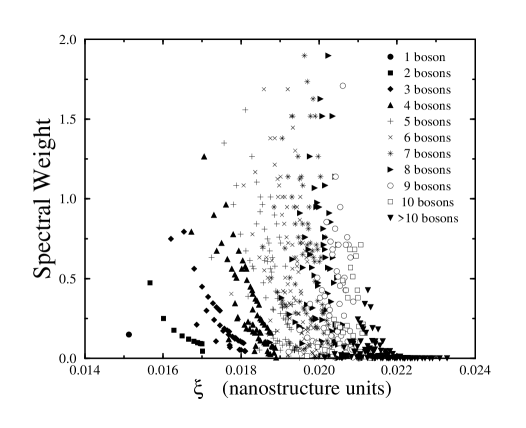
FIG. 1.: Structure in the spectral function (13) for fixed $Q=20$. Shown are the weights of the peaks in ${\cal A}(Q,\xi)$ as a function of the energy $\xi$ (unit: $\frac{e^{2}}{\epsilon\ell\pi}\sim 4.4\,$meV at 10 T) at which they are located. Data points denoted by the same symbol represent states with the same total number of bosons $\aleph$ in the system. Indicated are peaks for $\aleph=1,2,\dots,10$. These results are for $\nu=1/3$ and $R=2500\ell$. At typical fields this corresponds to $R\sim 20\mu$m.

For the realistic long-range interaction case, however, it is necessary to expand the exponential in Eq. (8) before Fourier transforming. For a given value of $Q$ we obtain a separate delta function in energy for each way in which the integer $Q$ can be expressed as a sum of integers, thus relating the spectral function calculation to the mathematical theory of partitions[39]. A partition of an integer $Q$ is a decomposition of $Q$ into the sum of integers $n\leq Q$: $Q=\sum_{n}n\,l_{n}$ where each integer $n$ occurs $l_{n}$ times. Partitions are usually specified by the symbol $(l)\equiv(1^{l_{1}}2^{l_{2}}\dots Q^{l_{Q}})$. Using this notation, we can write

$${\cal A}(Q,\xi)=z\sum_{(l)\mbox{~{}of }Q}w^{(l)}_{\nu}\,\,\delta\big{(}\xi-E^{(l)}\big{)}$$ (13)

where the sum is taken over all partitions $(l)$ of $Q$, and the expressions for the weights $w^{(l)}_{\nu}$ and energies $E^{(l)}$ are

$$w^{(l)}_{\nu}=\left[\prod_{n\in(l)}(\nu n)^{l_{n}}l_{n}!\right]^{-1}$$ (14)

and

$$E^{(l)}=\sum_{n\in(l)}l_{n}\,E(n/R)$$ (15)

respectively. For small $Q$ all partitions are readily enumerated and expressions (14) and (15) evaluated. In Fig. 1 we show the 627 peaks which occur in the spectral function for $Q=20$.

The formal structure of expression (13) can be understood by noting that, for fixed $Q$, each partition $(l)$ is uniquely related to a microscopic many-particle state. The strength $w^{(l)}_{\nu}$ of the contribution of a particular state represented by the partition $(l)$ to the spectral function is proportional to the probability that the state created by adding an electron to the edge of a QH system will have total excess momentum $Q/R$ and $l_{n}$ bosons with momentum $n/R$. The excitation with the smallest energy possible at wavevector $q=Q/R$ gives rise to a $\delta$-function peak at $\xi=\xi^{\mbox{min}}_{q}=E(q)$ and corresponds to the state with exactly one boson with momentum $q$ in the system (cf. left-most symbol [filled circle] in Fig. 1). The largest excitation energy $\xi^{\mbox{max}}_{q}$ occurs for the state with $Q$ bosons of momentum $1/R$, represented by the right-most symbol (triangle down) in Fig. 1:

$$\xi^{\mbox{max}}_{q}=E(q)\left[1+\frac{\ln(qR)}{\ln(1/\alpha\,q\ell)}\right]\mbox{ .}$$ (16)

The total number of bosons for a state represented by partition $(l)$ is $\aleph=\sum_{n\in(l)}l_{n}$. In Fig. 1, data points with the same symbol correspond to states with the same total boson number $\aleph$. The sum of all their weights is known from number theory[39]; it can be expressed in terms of the so-called Stirling numbers of the first kind[39] which are usually denoted by $S_{Q}^{(\aleph)}$. We observe that the peaks with large weight for states with fixed $\aleph$ cluster near the same energy $\xi_{\aleph}$. Furthermore, it is apparent from the figure (and easily understood formally) that the spectral weight of states with large $\aleph$ is small. However, the number of these states grows rapidly with $Q$. In order to estimate the line shape of the spectral function, we have to consider both the magnitude of the spectral weights for different states as well as the number of states available within a particular energy interval. We used the Stirling formula to approximately determine the partition $(l)_{\aleph}$ which maximizes the weight (Eq.(14)) for fixed $\aleph$. Since most of the peaks for fixed $\aleph$ cluster near $E^{(l)_{\aleph}}$, we propose the following approximate formula for the spectral function:

$$\tilde{\cal A}(Q,\xi)=z\sum_{\aleph=1}^{Q}\nu^{-\aleph}\frac{|S_{Q}^{(\aleph)}|}{Q!}\,\,\delta\big{(}\xi-E^{(l)_{\aleph}}\big{)}\mbox{ .}$$ (17)

Eq. (17) can be used to determine the energy at which the spectral function is peaked (for $qR>\nu^{-2}$):

$$\xi^{\mbox{peak}}_{q}\sim E(q)\left[1+\frac{\nu^{-2}}{qR}\,\frac{\ln(qR)}{\ln(1/\alpha\,q\ell)}\right]\mbox{ .}$$ (18)

In the case of short-range interaction, the effect of a fractional filling factor $\nu$ is to shift spectral weight towards higher energies. If the interaction is long-ranged, this effect is enhanced, and the suppression of spectral weight at low energies is effectively stronger. As the comparison of Eq. (18) and $\xi^{\mbox{min}},\xi^{\mbox{max}}$ shows, this enhancement is weakened at large $Q=qR$.

Recently, Luttinger liquid behavior of QH edges was observed in measurements of the IV-characteristics for tunneling from a reservoir into QH edges[18] and for tunneling between two co-planar edge channels[19].

FIG. 2.: IV-curve for tunneling from a particle reservoir into a QH edge ($\nu=1/3$, $R=2500\ell\sim 20\mu$m typically, corresponding to $10^{6}$ electrons). Inset shows step-structure resulting from finite size of the system. Step width in the voltage is non-uniform, which is a signature of Coulomb interaction. Nanostructure units: $[V]=\frac{e}{\epsilon\ell\pi}\sim 4.4$mV here.

In both experiments, translational symmetry was broken, and the tunneling process was not restricted by momentum conservation. We will show below that in experiments of this kind, the broadening of the spectral function due to the long range of Coulomb interaction (as discussed above) does not lead to easily observable effects. Instead, we propose an experiment which measures tunneling currents between two-dimensional electron systems[40, 41] displaced along their normals. This so-called vertical tunneling experiment is directly sensitive to the line shape of the spectral function.

According to standard theory[38] based on the tunneling Hamiltonian formalism, the expression for the IV-characteristics for tunneling between two systems (labelled by indices $U,L$, respectively) which are separated by a barrier is

$$I(V)=$$ (20)

$$2\pi e\sum_{k,p}\big{|}t_{kp}\big{|}^{2}\int_{\mu^{(U)}-eV}^{\mu^{(L)}}d\epsilon\,\,A^{(L)}(k,\epsilon)A^{(U)}(p,\epsilon+eV)$$

at zero temperature. If we consider tunneling from a reservoir into a QH edge, the tunneling amplitude will not importantly depend on momentum: $\big{|}t_{kp}\big{|}^{2}\sim t^{2}$. Eq. (20) then specializes to

$$I(V)=2\pi et^{2}\,{\cal N}\,\sum_{Q}\int_{0}^{eV}d\xi\,\,\,{\cal A}(Q,\xi)$$ (21)

where we assumed the reservoir’s DOS to be essentially constant ($\equiv{\cal N}$) and the chemical potential in both systems to be equal. As ${\cal A}(Q,\xi)$ is a sum of $\delta$-functions in the variable $\xi$, the integration is easily performed. The numerically-determined IV-curve is shown in Fig. 2. It turns out that, for experimentally realistic sample sizes, the IV-curve shows power-law behavior $I\sim V^{1/\nu}$ as predicted[13] for the short-range interaction case. The long range of Coulomb interaction manifests itself only in small corrections (logarithmic in the voltage) to the power-law. The reason is that a tunneling probe within the plane of the 2DES is sensitive only to the total spectral weight for energies below $eV$, and the width of the spectral functions becomes unimportant. Note that the smallest possible excitation energy (i.e. $E(1/R)$ ) is quite big even for large samples; typical numbers are $4.6\,\mu$eV ($0.14\,\mu$eV) for $R=20\,\mu$m (1mm) at 10T and $\nu=1/3$. This leads to the appreciable finite-size effects seen in the inset of Fig. 2 at low voltages. For a short-range interaction, the step-size in voltage would be uniform. It is a signature of the Coulomb interaction that the voltage step-size is irregular.

The situation is different if we consider tunneling between two QH edges which are separated vertically, i.e. belong to two different 2DES which are parallel to each other. As tunneling occurs now from/into the whole (1D) edges, momentum conservation severely restricts the tunneling process, and we have $\big{|}t_{kp}\big{|}^{2}\longrightarrow t^{2}\,\delta_{kp}$. For tunneling to occur, we have to create an excitation with momentum below the Fermi point in one system and an excitation above the Fermi point in the other at the same time. Therefore, in a vertical tunneling experiment, a nonzero current will occur at finite voltages only if the Fermi wavevectors $k_{F}^{(U)},k_{F}^{(L)}$ in the two systems are different: $(k_{F}^{(L)}-k_{F}^{(U)})R\equiv\tilde{Q}>0$. In other words, if the Fermi wavevectors in the systems $U,L$ are different, $k$-conservation does not mean $q$-conservation (remember: $k\equiv k_{F}+q$). Expression (20) can be evaluated analytically for vertical tunneling and yields

$$I(V)=2\pi et^{2}z^{2}\sum_{(l)\mbox{~{}of }\tilde{Q}}w^{(l)}_{\nu/2}\,\,\delta\big{(}eV-E^{(l)}\big{)}\mbox{ .}$$ (22)

This result means that, by tuning[42] the off-set in the Fermi wavevectors for the two vertically-separated edges, it is possible to explore the structure in the spectral function directly by measuring the tunneling IV-curve. The tunneling current (22) has peaks at voltages corresponding to the peaks in ${\cal A}(\tilde{Q},\xi)$. The weight of the peaks in the the IV-curve is simply related to the spectral weight of the corresponding peak in ${\cal A}(\tilde{Q},\xi)$. Hence the IV-curve for fixed $\tilde{Q}$ looks similar to Fig. 1. However, peaks at higher voltages will be enhanced even more strongly. In experiment, the broadening of each peak (due to electron-phonon coupling and disorder effects) has to be taken into account.

In summary, we have calculated the spectral function for electrons at quantum Hall edges with Coulomb interaction present. We quantify its finite width, and give expressions for tunneling IV-curves. Vertical tunneling provides a direct probe of the line shape.

The authors would like to thank S.M. Girvin, J.J. Palacios, and R. Haussmann for numerous useful discussions. This work was funded in part by the National Science Foundation under Grant No. DMR-9416906. U.Z. gratefully acknowledges financial support from Studienstiftung des deutschen Volkes (Bonn, Germany).

REFERENCES

- [1] A. H. MacDonald, in Proceedings of the 1994 Les Houches Summer School on Mesoscopic Physics, edited by E. Akkermans et al. (Elsevier Science, Amsterdam, 1995), pp. 659–720.
- [2] R. B. Laughlin, Phys. Rev. B 23, 5632 (1981).
- [3] B. I. Halperin, Phys. Rev. B 25, 2185 (1982).
- [4] A. H. MacDonald and P. Středa, Phys. Rev. B 29, 1616 (1984).
- [5] M. Büttiker, Phys. Rev. B 38, 9375 (1988).
- [6] V. J. Emery, in Highly Conducting One-Dimensional Solids, edited by J. T. Devreese et al. (Plenum Press, New York, 1979), pp. 247–303.
- [7] J. S\a’olyom, Adv. Phys. 28, 201 (1979).
- [8] F. D. M. Haldane, J. Phys. C 14, 2585 (1981).
- [9] W. Apel and T. M. Rice, Phys. Rev. B 26, 7063 (1982).
- [10] A. H. MacDonald, Brazilian J. Phys. 26, 43 (1996).
- [11] X. G. Wen, Phys. Rev. B 41, 12838 (1990).
- [12] X. G. Wen, Phys. Rev. B 44, 5708 (1991).
- [13] X. G. Wen, Int. Journ. Mod. Phys. B 6, 1711 (1992).
- [14] C. L. Kane and M. P. A. Fisher, Phys. Rev. B 46, 15233 (1992).
- [15] A. Furusaki and N. Nagaosa, Phys. Rev. B 47, 3827 (1993).
- [16] K. Moon et al., Phys. Rev. Lett. 71, 4381 (1993).
- [17] P. Fendley, A. W. W. Ludwig, and H. Saleur, Phys. Rev. Lett. 74, 3005 (1995).
- [18] A. M. Chang, L. N. Pfeiffer, and K. W. West, Phys. Rev. Lett. 77 (to appear).
- [19] F. P. Milliken, C. P. Umbach, and R. A. Webb, Solid State Comm. 97, 309 (1996).
- [20] H. J. Schulz, Phys. Rev. Lett. 71, 1864 (1993).
- [21] M. Fabrizio, A. O. Gogolin, and S. Scheidl, Phys. Rev. Lett. 72, 2235 (1994).
- [22] H. Maurey and T. Giamarchi, Phys. Rev. B 51, 10833 (1995).
- [23] Y. Oreg and A. M. Finkel’stein, Phys. Rev. Lett. 74, 3668 (1995).
- [24] M. Franco and L. Brey, Phys. Rev. Lett. 77, 1358 (1996).
- [25] K. Moon and S. M. Girvin, Phys. Rev. B 54, 4448 (1996).
- [26] U. Zülicke and A. H. MacDonald (unpublished).
- [27] V. A. Volkov and S. A. Mikhailov, Zh. Eksp. Teor. Fiz. 94, 217 (1988) [Sov. Phys. JETP 67, 1639 (1988)].
- [28] S. J. Allen, H. L. Störmer, and J. C. M. Hwang, Phys. Rev. B 28, 4875 (1983).
- [29] T. Demel, D. Heitmann, P. Grambow, and K. Ploog, Phys. Rev. Lett. 64, 788 (1990).
- [30] M. Wassermeier et al., Phys. Rev. B 41, 10287 (1990).
- [31] I. Grodnensky, D. Heitmann, and K. von Klitzing, Phys. Rev. Lett. 67, 1091 (1991).
- [32] R. C. Ashoori et al., Phys. Rev. B 45, 3894 (1992).
- [33] D. B. Mast, A. J. Dahm, and A. L. Fetter, Phys. Rev. Lett 54, 1706 (1985).
- [34] D. C. Glattli et al., Phys. Rev. Lett 54, 1710 (1985).
- [35] P. J. M. Peters et al., Phys. Rev. Lett. 67, 2199 (1991).
- [36] S. Giovanazzi, L. Pitaevskii, and S. Stringari, Phys. Rev Lett 72, 3230 (1994).
- [37] J. J. Palacios and A. H. MacDonald, Phys. Rev. Lett. 76, 118 (1996).
- [38] G. D. Mahan, Many-Particle Physics (Plenum, New York, 1990).
- [39] G. E. Andrews, The Theory of Partitions (Addison-Wesley, Reading, 1976); see also K. Schönhammer and V. Meden, Phys. Rev. B 47, 16205 (1993).
- [40] J. Smoliner, E. Gornik, and G. Weimann, Appl. Phys. Lett. 52, 2136 (1988).
- [41] J. P. Eisenstein, T. J. Gramila, L. N. Pfeiffer, and K. W. West, Phys. Rev. B 44, 6511 (1991).
- [42] A possible way to tune is to apply an in-plane magnetic field. By measuring the tunneling current, the experiment can be calibrated. At , the only peak in the IV-curve will occur at zero voltage. Having achieved this calibration, it is possible to set the in-plane magnetic field for accurately determining .