Synchronization of
Integrate and Fire oscillators with global coupling

Abstract

In this article we study the behavior of globally coupled assemblies of a large number of Integrate and Fire oscillators with excitatory pulse-like interactions. On some simple models we show that the additive effects of pulses on the state of Integrate and Fire oscillators are sufficient for the synchronization of the relaxations of all the oscillators. This synchronization occurs in two forms depending on the system: either the oscillators evolve “en bloc” at the same phase and therefore relax together or the oscillators do not remain in phase but their relaxations occur always in stable avalanches. We prove that synchronization can occur independently of the convexity or concavity of the oscillators evolution function. Furthermore the presence of disorder, up to some level, is not only compatible with synchronization, but removes some possible degeneracy of identical systems and allows new mechanisms towards this state.
PACS numbers: 05.20.-y+b,64.60.Cn,87.10.+e
LPTHE preprint 9604

1 Introduction

The emergence of a large scale rhythmic activity in dynamical systems with a high number of degrees of freedom is a widespread phenomenon occurring in different fields. In physics, macroscopic synchronization may be found in the behavior of laser [1], charged density waves [2, 3], networks of Josephson junctions [4, 5]. In Chemistry, oscillating chemical reactions are the result of large scale synchronized activity [6],[7]. Many biological systems display also large scale synchronization [8]. One of the most cited example is given by the south-eastern fireflies where a large number of insects gathered on trees flash altogether[9, 10, 11, 12]. Other examples are reviewed in [13] and include cells of the heart pacemaker, circadian neural networks, glycolytic oscillations in yeast cells suspension, collective oscillations of pancreatic beta cells, crickets that chirp in unison[14, 15]. Coherent oscillations are also believed to be important in neuronal activity [16, 17].

The previous systems exhibiting large scale periodic activity are usually modeled as a large assembly of coupled oscillators. The periodicity shown by the whole system is then the result of the collective synchronization of a macroscopic set of the elementary oscillators. Due to the large diffusion of collective rhythmic behavior in nature, it is important to search and investigate all the possible mechanisms that may lead to this phenomenon in populations of oscillators.

Most of the works related to collective synchronization in the last decade studied populations of stable limit cycle oscillators described by ordinary differential equations continuously coupled in time [18, 19, 20, 21, 22, 23, 24, 25, 26, 27]. Much theoretical understanding has been obtained for such systems, as well on models where the phases are the only relevant dynamical parameters [18, 19, 20, 21, 22, 23, 24, 25, 28, 29, 30] or on models where phase and amplitude can vary[26, 31, 27], and for populations of identical or almost similar oscillators. Generally, global coupling has been assumed, i.e. each oscillator is supposed to interact with all the others. Local interactions have also been investigated[23, 22, 20] showing more complex behaviors.

These numerous studies do not however account for the important case, especially in biology, of episodic pulse-like interaction, where oscillating units, cells or neurons, often communicate through the sudden firing of a pulse. Biological oscillators exchanging pulses are currently modeled as Integrate and Fire (IF) oscillators[32, 33] which are simply described by some real valued state variable – representing for example a membrane potential – monotonically increasing up to a threshold. When this threshold is reached the oscillator relaxes to a basal level by firing a pulse to the other oscillators and a new period begins. This is the case for example for fireflies communicating through light flashes [9, 10, 34, 11], for crickets exchanging chirps [14, 15], for cardiac cells interacting with voltage pulses [35] and for neurons receiving and sending synaptic pulses.

Large assemblies of oscillators with pulse-like coupling have been studied only recently. In their seminal work, Mirollo and Strogatz[36] prove rigorously that a population of identical Integrate and Fire oscillators globally coupled by exciting pulses added to the state variables can synchronize completely for a certain kind of oscillators (convex oscillators). As showed by Kuramoto[37] who gives a description of such a system in terms of a Fokker-Plank equation, the coherent collective synchronization persists when random noise is included in the system. Recently Corral et al.[38] have generalized the Mirollo and Strogatz model for arbitrary evolution function of the oscillators and arbitrary response function to pulses and established some conditions sufficient for synchronization. When transmission delays are taken into account, Ernst et al. [39] find that with excitatory pulses, clusters of synchronized oscillators spontaneously form but are unstable and desynchronize after a time; partial synchronization is however achieved with inhibitory pulses in the form of several stable clusters of oscillators in phase.

Other studies consider models of Integrate and Fire oscillators with the pulses smoothed before acting on the oscillator state variable[40, 41, 42]. Recently Hansel et al.[42] showed that rise and fall times can destabilize the synchronized state of simple IF oscillators and Abbott and van Vreeswijk [41] showed that in this case the incoherent asynchronous state can be stable. In a model with fall times of the coupling between the oscillators, Tsodyks et al.[40] showed that the complete synchronized state is unstable to inhomogeneity in the oscillators frequencies. Finally Gerstner [43, 17] achieved a synthesis of results on IF oscillators models by introducing a general model containing various versions of IF models as special cases and an analytical approach from the point of view of a renewal theory [44, 45, 46]. In the previous studies the oscillators are typically model neurons described as leaky integrator on a membrane potential. This assumption determines the form of the monotonic variation function of the state variable of the free oscillators which in this case must be convex.

In this article we extend a previous study [47] of IF oscillators with linear or concave variation and with a global all to all excitatory pulse coupling directly added to the oscillator state variables. According to the theorem of Mirollo and Strogatz[36] it was commonly believed that synchronization of pulse coupled IF oscillators could be achieved only with convex oscillators. We show here that actually synchronization can occur independently of the shape of the oscillators which is not therefore a constraint for this behavior. We present and investigate some general mechanisms that, we think, have not been sufficiently recognized previously and that lead to collective synchronization in assemblies of linear oscillators without or with quenched disorder. These effects, sufficient for synchronization for linear oscillators, can also exist for models of leaky integrator oscillators and be combined with other mechanisms.

The aim of this paper is not to study a particular biological or physical phenomenon in details but to get a better understanding of the possible mechanisms of mutual entrainment that can lead to collective synchronization in models of IF oscillators. Furthermore, systems of simple linear oscillators of the kind studied in this article are also found in a different context than collective synchronization, which is the physics of earthquakes and Self-Organized Criticality [48]. This phenomenon is the spontaneous organization of a dynamical system with a large number of degrees of freedom out of thermodynamical equilibrium, in a critical, i.e. scale invariant, state of evolution which is attractor of the dynamics. The building up of the long range correlations and power law behaviors characteristic of the critical state does therefore not require the fine tuning of a control parameter (temperature, magnetic field, etc…) as for the usual critical phenomenon of second order phase transitions. Famous examples of dynamical systems with a high number of degrees of freedom believed to be self-organized critical are for example the sandpile model of Bak, Tang and Wiesenfeld [48] together with several variants [49, 50, 51], a model of front propagation [52], evolution models for species[53], the forest-fire model[54], etc…Self-Organized Criticality has also raised interest in Geophysics as a possible phenomenon responsible for the scale invariant behavior of earthquakes, whose distribution of their number as a function of their magnitude (Gutenberg-Richter distribution) is a power law.

A classical model of earthquakes is the Burridge-Knopoff spring-block model, where the fault between two tectonic plates is described as a network of rigid blocks elastically connected and coupled semi-elastically and semi-frictionally to the surfaces of the fault. Due to the relative movement of the tectonic plates, the stresses on all the blocks increase until the stress of some block reaches an upper threshold and relaxes causing the slipping of the block and a rearrangement of the constraints on the neighboring blocs. This can possibly push other blocks to relax and trigger an avalanche of slippings, i.e. an earthquake. As first noticed by Christensen [55], the previous systems can be seen as assemblies of pulse coupled oscillators: each block is actually an oscillator with the stress upon it acting as the state-variable and the pulses being the sudden increment of the strain on the neighbors of the slipping bloc. A discretized version of the Burridge-Knopoff model by Olami, Feder and Christensen[56] with linearly varying oscillators, nearest neighbors coupling and direct action of the pulses on the state variable is believed to be self-organized critical. It has been proposed [55, 57, 58, 47, 59] that the critical behavior of this model is related to the tendency to synchronization in such systems. In this article we see that the globally coupled models, which are actually mean-field versions of the Olami-Feder-Christensen model, are not critical and typically synchronize.

This paper is organized as follows: In sections 2.1 and 2.2 we show that because of a positive feedback of large groups of synchronized oscillators on smaller ones, complete synchronization of a set of identical oscillators is possible even in cases not taken into account by the theorem of Mirollo and Strogatz [36]. In section 3, we show how the introduction of disorder on the oscillator properties such as the frequencies, the thresholds or the pulse strengths allows a new mechanism that can lead to collective synchronization. Two effects act together: first, the quenched disorder makes the effective rhythms of the oscillators all different. This brings any two oscillators to relax time to time simultaneously. Second, oscillators that fired simultaneously possibly remain locked in a synchronized group. Finally, in the last section4, we discuss our results focusing especially on the effects of convexity, linearity or concavity of the oscillators state variation function, on additivity or not of the pulses, on refractory time after a relaxation and on the possible kinds of synchronization.

1.1 Models

In this article we study models of $N$ IF oscillators $O_{i},i=1\dots N$ represented by a real state variable $E_{i}\in[0,E_{i}^{c}],i=1\dots N$, where the $E_{i}^{c}$ are the thresholds of the oscillators. The free evolution of $O_{i}$ is made of two parts: first, a charging, growth, period where the state variable $E_{i}$ increases monotonically in time as long as it is below the threshold $E_{i}^{c}$ according to a given free evolution variation function $E_{i}(t)$ and, second, a relaxation when the threshold is reached whereby $E_{i}$ is reset to zero and a growth period starts again. We assume, as it is generally done, that the characteristic time for the relaxation is very short compared to the period of the free evolution so that the state variable $E_{i}$ of an oscillator that fires is instantaneously reset to zero.

It is convenient to introduce the phases of the oscillators defined as $\phi_{i}\equiv t\ {\rm mod}\ \phi_{i}^{c}$ where $\phi_{i}^{c}$ is the free period of $O_{i}$ ($E_{i}(\phi_{i}^{c})=E_{i}^{c}$).

The coupling between biological oscillators, for instance fireflies, has been experimentally studied by perturbing the oscillating elements by single pulses [60, 33]. Knowing that fireflies interact through light flashes and that they are believed to be describable by coupled IF oscillators [9, 36], the interaction between the oscillators is studied by observing the response of the periodic flashing of a single firefly to an artificial flash [9]. Following such studies several types of couplings have been introduced in biological models involving IF oscillators. In the situations under interest, an oscillator is coupled with others when it relaxes and the coupling takes the form of a pulse transmitted to the others. The consequences of the firing on the oscillators that have received the pulse depend on the biological situations and on the models.

Pulses may be excitatory, i.e. incrementing the state variables and thus anticipating the firing of the receiving oscillators, or inhibitory, i.e. decrementing the states and delaying the firing of the receivers.

In this article we consider excitatory pulses:

1. An oscillator receiving a pulse has its state variable incremented by the pulse strength. This model of coupling is known as phase advance model since the pulses push the oscillators towards their thresholds – and possibly above – causing a sudden advance of the phases of the oscillators on their period of evolution.

2. The pulse strength depends on the number of oscillators that fire together and obey an additivity principle: the pulse from the simultaneous relaxation of oscillators is an increasing function of the sum of all the individual pulses of the firing oscillators. For the sake of simplicity we assume in this article direct additivity: the simultaneous firing of $n$ oscillators transmits a pulse of strength $n\delta$, with $\delta$ the pulse strength of a single oscillator. To account for the global coupling, $\delta$ scales as the inverse of the system size: $\delta=\alpha E_{c}/N$ with $\alpha$ a dissipation parameter.

2 Identical oscillators

In this section all the oscillators are identical: $E_{i}(t)=E(t),\ \forall i$ and the pulses have the same strength. We first study the case of linear $E(t)$ which corresponds to the limit of zero convexity of the model of Mirollo and Strogatz [36].

2.1 Linear oscillators

Between two firings, the state variable increases linearly. Without loss of generality we take simply $E_{i}(t)=t\ {\rm mod}\ E_{c}$ so that $0\leq E_{i}\leq E_{c}=1$. Most studies do not consider a linear variation of the state. Indeed the oscillators are commonly leaky integrators whose evolution between two firings is described by the differential equation:

$$\frac{dE_{i}(t)}{dt}=S_{0}-\gamma E_{i}\ \ \ \ \ ,\ \ \ \ \ 0\leq E_{i}\leq E_{c}=1,$$ (1)

where $S_{0}$ is a constant input current and $\gamma$ describes the dissipation. The solution of this differential equation is a convex function with the convexity controlled by the dissipation $\gamma$.

Mirollo and Strogatz[36] have rigorously proved that with $\gamma>0$ and with constant pulses a population of oscillators always synchronizes. From their theorem the convexity seemed to be a necessary condition for synchronization. However, as first noticed by Christensen [55], a large set of oscillators with linear evolution may effectively synchronize completely.

As we shall see, the convexity is a sufficient but not necessary condition for synchronization. Convexity implies that the increment of the phase of an oscillator due to a pulse increases as the oscillator is nearer to the threshold, which has the consequence that two oscillators effectively attract each other in the course of time.

We show in the following that simply due to the hypothesis of additivity of pulses there is a positive feedback effect towards synchronization in the system, which is not necessary in the convex case for the validity of the theorem of Mirollo and Strogatz. We prove that this effect is sufficient for synchronization even on sets of linear and concave oscillators. Let us first introduce the notions of avalanche and of absorption that will be important in the following.

Avalanches.

An avalanche of successive firings may occur when an oscillator reaches the threshold: depending on the other oscillator states the transmitted pulse may bring some other oscillators to exceed the threshold and to fire. Possibly the new pulses may themselves cause further relaxations and a cascade of firings until no more pulse is sufficient to bring another oscillator above the threshold. In this study, we assume that the firings and that their transmission are very fast compared to the free evolution period of the oscillators so that during an avalanche the continuous drive of the oscillators is not acting.

Avalanches are also important for the link with the models on lattices showing Self-Organized-Criticality, which will be discussed elsewhere [61].

Absorption rule and definition of synchronization.

As can be seen on fig.1 in the model defined up to now, oscillators can never get in phase. A supplementary rule, that exists also in the model of Mirollo and Strogatz, and that we call rule of absorption is necessary for that. Since the oscillators synchronize through the firings, we can assume, that the oscillators get in phase when they fire in a same avalanche.

Figure 1: Evolution without absorption. Values of the states of two identical oscillators with convex variation. a. The oscillator (1) is at the threshold, the oscillator (2) is below the threshold at a distance smaller than $\delta$ which is the pulse strength of a single firing. b. The oscillator (1) has relaxed and the emitted pulse has pushed the oscillator (2) above the threshold and makes it fire in avalanche. c. Without absorption the firing of oscillator (2) has pushed (1) away from the origin: the oscillators remain dephased independently of the convexity.

We say that they are absorbed in a synchronized group of oscillators with identical phase. Absorption is implemented naturally by assuming that the oscillators that relax during an avalanche are insensitive to the further pulses in the avalanche and remain until it ends at zero value. This rule corresponds actually to a refractory time of the oscillators immediately after their relaxation. Absorption is necessary for oscillators to get in phase and possibly to evolve thereafter synchroneously with the same phase. However, it is possible to have a different definition of synchronization in models of pulse coupled IF oscillators than evolution in phase, that does not require the absorption rule. This is synchronization as locking into avalanches. Since we assume a separation of time scales between fast firings and slow continuous variation of the state variables, locking in avalanches corresponds, on the scale of the free oscillator period, also to a real synchronization of avalanches in time. Consider in the model without absorption two oscillators that fire in the same avalanche as in fig.1, due to the second firing their state are different by the value $\delta$, the pulse strength of a single oscillator. When the most advanced oscillator is back to the threshold (fig.2), the difference between the values of the state variables is smaller or equal to $\delta$, in the case respectively of convex or linear oscillators.

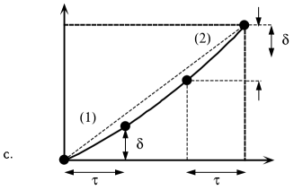
Figure 2: a. Synchronization without absorption for identical convex oscillators. 1) Immediately after their avalanche two oscillators $O_{i}$ and $O_{i-1}$ have a gap between their states $E$ of value $\delta$. $\tau$ is the gap between the phases of $O_{i}$ and $O_{i-1}$, which does not change during the free evolution between firings. 2) When the most advanced oscillator is at the threshold the gap between their phases has not changed but the gap between their state variables has decreased due to the convexity. The second oscillator is at a distance of the threshold smaller than $\delta$: the oscillators avalanche again together. b. Synchronization without absorption for identical linear oscillators. Same as for the convex case, but due to the linearity the gap between the states values does not change and is exactly equal to $\delta$: the oscillators still avalanche together. c. Effect of concavity. The gap between the oscillators states increases as the pair approaches the threshold.

In both cases the pulse from the next firing is sufficient to push the second oscillator above or exactly at the threshold and therefore to make it fire also: the two oscillators are again in a same avalanche. We see that if two oscillators come at some time to avalanche together they will thereafter continue to fire always together in the same avalanche also without absorption. It is therefore sensible to speak of synchronization also in such a case of locking of the firings in a same avalanche. We shall discuss in the rest of the paper what kind of synchronization is possible for the different models. For systems of identical oscillators we can see on fig.2 that locking in avalanches is possible for convex or linear variation functions but not for concave oscillators. Phase synchronization is in some cases equivalent to synchronization as locking in avalanches. Suppose that phase synchronization occurs in a model $A$ with the absorption rule. If in the version $B$ of the same model, but without absorption, oscillators that are in a same avalanche remain locked, then both models $A$ and $B$ evolve in the same way, where the same oscillators that are synchronized with identical phase in model $A$ are locked in an avalanche in model $B$. Therefore if complete synchronization occurs in models $A$ then complete synchronization occurs also in model $B$ without absorption in the form of locking of all the oscillators in a stable avalanche. For simplicity we choose to include absorption in this section on linear oscillators (here without loss of generality) and in the following on concave oscillators ( then necessary for synchronization).
– Proof of synchronization
Let us call configuration the set of ordered distinct values $E_{1}^{(k)}<E_{2}^{(k)}<\dots<E_{m_{k}}^{(k)}=1$ of the state variables present in the system just before the $(k+1)$-th avalanche. To each $E_{i}^{(k)}$ corresponds a group $G_{i}$ of $N_{i}^{(k)}$ oscillators at this value and $\sum_{i=1}^{m_{k}}N_{i}^{(k)}=N$. Let call cycle, the time necessary for all the $m_{k}$ groups to avalanche exactly once. To trace the evolution of the system, it is useful to follow, cycle after cycle, the gaps $s_{i,j}^{(k)}=E_{i}^{(k)}-E_{j}^{(k)}$ between the values of two groups. If one of these gaps $s_{i,j}^{(k)}$ becomes smaller than the value $N_{i}^{(k)}\delta$ of the pulse of the $(i)$-th group, then the $(j)$-th group gets absorbed by the $(j)$-th group. On table 1 we find the main steps of the variation of the gap $s_{i,j}^{(k)}$ on a cycle beginning with $G_{i}$ at the threshold. Since the oscillators are identical and linear, both groups have the same evolution as long as neither $G_{i}$ nor $G_{j}$ relax: they get the same pulses from other relaxations with the same phase advances and between pulses their state variables increase at the same rate.

$$\mathbf{G_{i}}$$

a.

b. 0

c.

d.

e.

Table 1: a. Beginning of a cycle with the group $G_{i}$ at the threshold, the group $G_{j}$ is at a distance $s_{(i,j)}^{(k)}$. b. Firing of $G_{i}$. c. $G_{j}$ is at the threshold. d. firing of $G_{j}$. e. End of the cycle $G_{i}$ is back at the threshold.

From table 1 we see that the first return map on a cycle for the gap between the oscillators is then:

$$s_{i,j}^{(k+1)}=s_{i,j}^{(k)}+(N_{j}-N_{i})\delta.$$ (2)

If $N_{i}>N_{j}$ the gap between the two groups decreases on each cycle. When the difference between the states $E_{i}$ and $E_{j}$ becomes less or equal to $N_{i}\delta$, then the relaxation of $G_{i}$ drags $G_{j}$ along in an avalanche. Due to the absorption, both groups then form a greater group with $N_{i}+N_{j}$ elements. The growth of groups is therefore due to a positive feedback mechanism where the larger groups attract the smaller ones. This effect exists only if there are in the population groups of different sizes. We shall now see that as long as the number $N$ of oscillators is sufficiently large, positive feedback always occurs until complete synchronization of the system. If the evolution of the system begins with random initial phases for all the oscillators, all the $E_{i}$ are different: there are no groups and one could naively expect no positive feedback and no evolution towards synchronization. However some groups are naturally formed in the first cycle of the evolution. Indeed if two oscillators happen to be sufficiently close to each other, i.e. $E_{i+1}-E_{i}$, the pulse from the first of them drags the other in an avalanche and a group of two is formed. Thereafter there are in the system single oscillators and a group of at least size two, so that the positive feedback mechanism can proceed. In order to see how probable a uniform random initial configuration leads to the feedback effect we must therefore estimate the probability that at least two $E_{i}$ are separated by less than $\delta$ in a set of $N$ random numbers between zero and $E_{c}$. The probability $P(s)ds$ that two random numbers among $N$ in $[0,E_{c}]$ are separated by a distance between $s$ and $s+ds$ is given in the limit $N\gg 1$ by a Poissonian:

$$P(s)ds=\frac{N}{E_{c}}e^{-\frac{N}{E_{c}}s}ds.$$ (3)

The number of gaps between initial random values satisfying the condition for formation of a pair is then:

$$N\int_{0}^{\frac{\alpha}{N}}P(s)ds=N(1-e^{-\frac{\alpha}{E_{c}}})\ \ \ \ \ \ ,\ \ \ \ \ \ N\gg 1.$$ (4)

Positive feedback and the absorption of oscillators into groups may take place as long as there is at least one such a gap. It follows directly from (4) that this is typically the case if $\alpha/E_{c}\geq 1/N$. For a given level of conservation, the number of oscillators needs only to be large enough to ensure the onset of positive feedback.

Initial configurations where no gap is smaller than $\delta=\alpha E_{c}/N$ are in principle possible. However for large systems their occurrence is exponentially small: each gap has for $N$ large a probability $e^{-\alpha}$ of being greater than $\delta=\alpha/N$, so that the probability that all the oscillators are too far apart for pair formation goes as $e^{-\alpha N}$. Therefore we may conclude that the set of initial configurations that do not lead to absorptions is formed of extremely improbable configurations.

To complete the proof that synchronization is the general behavior of our model, we would need to show that the set of initial conditions for which the system evolves in a partially synchronized configuration where positive feedback stops acting is of almost vanishing measure. As we have seen with the equation (2), this can happen only when all groups are of equal size. It is a difficult task to calculate in general the probability for a random initial configuration to finally get stuck in such a state. In any case, this is a physically ill-defined problem since this probability depends critically of the multiples of $N$: would $N$ be prime, then for every initial condition forming at least an initial group of two the system would unavoidably synchronize completely.

Numerical simulations show that for increasing $N$ the probability for incomplete synchronization decreases. For example with a conservation level $\alpha=0.2$ we found for $N=200,400,1000$ incomplete synchronization in respectively $0.26,0.2$ and $0.05$ percent of the cases for $12000$ different initial configurations. For $N=5000$ we obtained always complete synchronization. When the synchronization was only partial the final state of the system was always made of only two groups of equal size $N/2$. For $N$ not divisible by two we found always complete synchronization. We see that the conditions for the existence of positive feedback are almost always fulfilled.

We studied the time necessary for synchronization numerically. Fig. 3 shows the distribution of the durations of the transient $T_{S}$ until complete synchrony for $N=2000$ and $\alpha=0.1,0.2,0.5,0.8$. The mean time for synchronization increases only slowly with the population size as a power law with exponent $\sim 0.13\pm 0.01$.

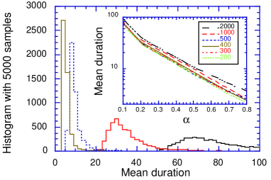
Figure 3: Binned distributions of the times for synchronization for a population of $N=2000$ linear oscillators with random uniform initial phases, with conservation level $\alpha=0.8,0.5,0.2,0.1$ and over a sample of $5000$ simulations; the time unit is the free period. Inset: Mean duration $T_{S}$ to synchronization as a function of $\alpha$ for different population sizes, $T_{S}\propto\exp{-(4.3\pm 0.2)\alpha}$.

The distributions have a flat tail towards long times corresponding to configurations where two groups of almost similar size remain in the system making the positive feedback effect weak and slow to achieve the merging of the groups. The inset of fig.3 shows $T_{S}$, calculated by cutting the tail of the distributions, as a function of $\alpha$ for $N=200,300,400,500,1000,2000$. The duration of the transient $T_{S}$ decreases with larger conservation level and for $\alpha\in[0.2,0.8]$ the decrease is exponential: $T_{S}\propto\exp{-(4.3\pm 0.2)\alpha}$. Synchronization occurs then quite fast in a few free periods. The duration of the transient $T_{S}$ depends on the additivity of pulses. Here we assumed perfect additivity, however if the effect of the firing of a group is not simply the sum of all the single firings but a smaller function of their number, we expect some longer synchronization time. We conclude that for large $N$ synchronization is possible and occurs in a finite time even for oscillators with a linear variation which were excluded by the theorem of Mirollo and Strogatz [36]. This theorem and the older results of Peskin [35] have been often erroneously interpreted as the necessity for synchronization of a “leaky” dynamics of the oscillators, which is related to the assumption of a convex variation function $E(t)$. Let us however stress that the demonstration in [36] for convex oscillators proves complete synchronization in this case for any initial configuration apart a set of Lebesgue measure null and is also valid without additivity of the pulses. In the case of convex oscillators the positive feedback mechanism is not necessary for synchronization. Additivity of pulses and the positive feedback mechanism that results is a further powerful mechanism which allows synchronization under broader conditions than the effect of convexity.

Our results with linear oscillators prove that leaky oscillators are not necessary for the phenomenon of synchronization and that other kinds of pulse coupled oscillators can be considered. As we show now, the form of the state variation function $E(t)$ is actually not even a constraint for synchronization since this phenomenon occurs also for concave $E(t)$.

2.2 Concave oscillators

For the sake of simplicity we choose as concave function for the evolution in time of the state variable of the oscillators a function of the form $E(t)=f_{a}(t)=t^{a}$, with $a>1$. The effect of the concavity on the relative state of two oscillators may be seen on fig.2c. Two oscillators $O_{i}$ and $O_{i+1}$ with phase difference $\tau$ see the difference $E_{i+1}(t)-E_{i}(t)$ increase as they approach the threshold. Therefore with large concavity it is more difficult that a pulse of an oscillator triggers an avalanche. However nothing forbids a group of oscillators to synchronize if, when the first oscillator reaches the threshold, the gaps between them are smaller than the pulse strength.

Compared with the previous case of a linearly increasing $E(t)$, we see that now the effect of positive feedback is opposed by the drawing apart effect of the concavity. In a first step we will see that for small concavity the positive feedback effect prevails and that synchronization occurs. Although one would expect that for larger concavities groups would not be able to grow, we will see in a second step that for systems starting their evolution with an initial random distribution of the oscillator phases, large concavities have the surprising consequence to favor actually the synchronization.

Small concavity $a\succeq 1$

We consider first the case of concave functions $E(t)$ that are close to the linear case. For clarity we only sketch here the main steps of the demonstration and refer to the appendix A for details and for the complete demonstration. We show there that for a random initial configuration of $N$ oscillators groups begin to form and grow by positive feedback as in the case of linear oscillators. However when only a few groups remain the positive feedback is sufficient to reduce the phase gaps between the groups and to cause further synchronization only if the size differences of the groups are large enough. The most difficult situation for the occurrence of synchronization is when only two groups remain in the system, say $G_{1}$ and $G_{2}$ with respectively $N_{1}$ and $N_{2}$ oscillators $(N_{1}>N_{2})$. There is then a limit value $\bar{c}$ of the size difference $c$ between $G_{1}$ and $G_{2}$ so that complete synchronization occurs only if $c=N_{1}-N_{2}>\bar{c}(a,N,\alpha)$. That is absorption occurs only if the size difference between the two groups is sufficiently large so that the positive feedback attraction between the groups is strong and can overcomes the effect of concavity. Contrary to the case of linear oscillators, we see here that two groups of different sizes – not only of equal sizes – may remain apart and not synchronize. This is the consequence of the drawing apart effect of the states by the concavity (fig.2c). Since $\bar{c}(a,N,\alpha)$ is a monotonically increasing function of $a$, for larger concavities less final configurations synchronize completely (for large concavities however another effect leading to synchronization can occur, see later).

For a given $N$ there is a finite value $\bar{a}$ of the concavity so that $a<\bar{a}\Rightarrow\bar{c}<1$. That is, for concavities smaller than $\bar{a}$ the system synchronizes completely unless the two last remaining groups are of equal sizes, which is the same condition than in the linear case. $\bar{a}$ goes to one as $1/N$ so the corresponding range of concave functions is quite small. We find however that synchronization occurs in practice also for much larger concavities with high probability.

The probability $\cal{P}$ of synchronization corresponds to the probability that the gap $c$ between the two last groups is larger than $\bar{c}$. Unfortunately it is difficult to calculate this probability directly. However we can estimate $\cal{P}$ by assuming simply a uniform distribution of $c$ in $[0,N]$. This assumption is natural since we start the evolution with a uniform initial distribution of the oscillator phases. $\cal{P}$ is then the ratio of the number of favorable cases, $N-c$, over $N$, the number of possible values of $c$. Using the value (17) of $\bar{c}$ calculated in the appendix A we get:

$${\cal P}=1-\frac{(1-a)}{2\alpha a}\left(\left(1-\frac{\alpha}{2}\right)\ln\left(1-\frac{\alpha}{2}\right)+\frac{\alpha}{2}\ln\left(\frac{\alpha}{2}\right)\right)+o\left(\left(\frac{1-a}{a}\right)^{2}\right).$$ (5)

Thus, the probability of synchronization is independent of the system size. On Table 2 we summarize the results of simulations obtained with $2000$ samples, for $\alpha=0.5$ and several levels of concavity. We indicate also the probabilities of synchronization expected with the assumption of uniform distribution of the size difference of the two last groups.

a $$\mathbf{1.005}$$

i.

ii.

Table 2: i. Probabilities of complete synchronization with the statistical error obtained with $2000$ samples for $\alpha=0.5$ for “small” concavities $a=1.005,1.05,1.1$. The probabilities obtained with $N=2000,1000,500,400,300,200$ are identical within the error. ii. Estimated probabilities of complete synchronization with the assumption of uniform distribution of the size difference between the two last groups in the system.

Within the statistical error the probabilities of synchronization are independent of $N$ and correspond to the expectations.

For small concavities $a=1.005,1.05,1.1$ we found that the duration $T_{S}$ of the transient until synchronization does not depend on the value of the concavity. In fig.4 we report the distributions of $T_{S}$ for $a=1.05$. It can be seen that typically synchronization occurs in a few free periods.

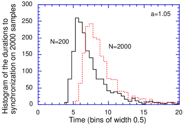
Figure 4: Binned distributions of the duration $T_{S}$ of the transient until complete synchronization in a population of $N=2000$ identical concave oscillators with concavity $a=1.05$ for $2000$ samples of uniformly distributed random phases.

Furthermore $T_{S}$ increases only slightly with the population size as a power law with a small exponent: $T_{S}\propto N^{0,09\pm 0.01}$ for $N=200$ to $2000$ and $\alpha=0.5$. Large populations synchronize therefore quite fast as in the linear case.

From what precedes we would expect that synchronization is impossible for large concavities. Without entering into details we shall now see that assuming a natural uniform initial distribution of the oscillators phases (and not of the states $E_{i}$) there is for large concavities a cross-over in the behavior of the system towards easier synchronization.

Large concavities

Let us first illustrate the mechanism at work on an extremely simplified model shown on fig.5a. where we replace the concave function by the union of its tangent segments at both extremities.

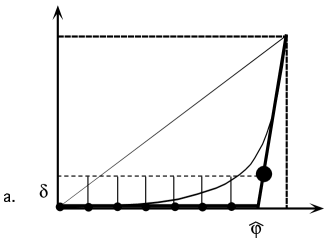
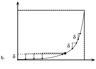
Figure 5: a.“Extremal” model with very large concavity. The state value evolution function is flat up to some phase $\hat{\phi}$ where it abruptly monotonically increases up to the threshold. All the oscillators with initial phase smaller than $\hat{\phi}$ have the same state value. They synchronize at the same phase value as soon as they receive any pulse $\delta$. b. For a large concavity $a$ but with a smooth state value evolution function $E(t)=f_{a}(t)$, the oscillator with small initial phases have also very close initial states. A pulse $\delta$ brings them at almost the same phase.

That is the free evolution function of the oscillators is now:

$$E(\phi)=\left\{\begin{array}[]{ll}0&,\phi\in[0,\frac{1}{a-1}]\\ (a-1)\phi+1&,\phi\in[\frac{1}{a-1},1]\end{array}\right.$$ (6)

with $a>1$. All the oscillators with initial phases in $[0,1/(a-1)]$ have the same initial state value $E_{i}=0$ due to the special form of the evolution function. It is clear from fig.5a that all these oscillators get in phase and synchronize as soon as the first pulse of the evolution occurs. It is then possible to show that the large synchronized group that is thus formed absorbs thereafter the oscillators that where initially in $[1/(a-1),1]$ and the system synchronizes completely.

For smoother $E(t)$ the same mechanism occurs (see fig.5b). For small phases $\phi\rightarrow 0$ the slope of the evolution function is small and thus the $E(\phi)$ are closer to each other than for larger phases where the slope is steeper. If the initial packing of the states subsists until one of the closely packed oscillators is at the threshold a large avalanche occurs and thus the synchronization of many oscillators. It is not obvious that the states remain close to each other. Indeed during the free evolution of the system (between firings) the gaps between the phases do not change but the states get farther apart from each other due to the concavity. On the opposite, during firings the gaps between the states remain constant since all the states are incremented the same way (whereby the phase gaps get smaller). Let the oscillators be numbered by increasing order of their initial phases $\phi_{i+1}^{(0)}>\phi_{i}^{(0)}$. The evolution of $O_{i}$ towards the threshold is caused as well by free evolution between avalanches as by phase advances due to pulses. Before reaching the threshold, an oscillator $O_{i}$ receives $N-i$ pulses from the oscillators with larger initial phases. For small initial phases $(i\rightarrow 1)$ the oscillators $O_{i}$ and $O_{i-1}$ receive many pulses and their evolution towards the threshold is for a large part due to the phase advances from pulses. Possibly there is sufficient evolution due to pulses so that the state gaps do not increase enough due to the free evolution to prevent a large avalanche of the initially closely packed oscillators.

a $$\mathbf{500}$$ estimate

Table 3: i. Probabilities of complete synchronization with the statistical error for “large” concavities $a=1.55$ and $a=2$ with $N=500,1000,2000$ and an a uniform initial distribution of the phases. The last column right shows the probabilities expected as for small concavities.

On Table (3) we see that for concavities $a=1.55$ and $a=2$ synchronization already occurs with a larger probability that expected with the estimate from small concavities. As expected the probability for synchronization increases with $a$ for a given population size $N$. We see also that the probability increases with $N$. This is the consequence that with a uniform distribution of phases the oscillators are at the beginning denser for larger populations in the flat section of $E(\phi)$ and larger synchronized groups form at the beginning of the evolution thus enhancing the positive feedback. Large concavities favor synchronization only for a uniform distribution of the initial phases. Indeed if, instead of the phases, the states $E_{i}$ of the oscillators were initially uniformly distributed in $[0,1]$, there would be, per definition, no clustering and the oscillators would stay apart, as it is easy to verify looking at fig.5a. An initial uniform distribution of the phases is however a natural assumption for the beginning of the evolution.

Finally, the main conclusion of this section is that surprisingly the form of the oscillator state variation function $E(\phi)$ is not actually relevant for synchronization that occurs with high probability for functions $E(\phi)$ which are convex, linear and even concave provided the phases are randomly distributed initially. The usual interpretation of “leakiness” (implying convexity) as a requirement for synchronization must therefore be revised. Up to now we have considered only identical oscillators. In the following sections we show that in populations of oscillators with different randomly distributed characteristics, synchronization occurs also in a different way that what we have seen up to now.

3 Systems with quenched disorder

We shall see that with quenched disorder, synchronization is the combined consequence of several causes. For the sake of simplicity we show how synchronization occurs in the cases of oscillators with respectively different free frequencies then different amplitudes and finally of oscillators with different frequencies and amplitudes. The mechanisms at work are the same for the different kinds of disorder although some important peculiarities depend on the models. In brief, these mechanisms and the main steps of the demonstrations are the following.

We write the first return map for the phase of a given oscillator $O_{j}$ on a cycle beginning and finishing when another given oscillator $O_{i}$ is at the threshold. During such a cycle all the oscillators of the system fire once. The first return map shows that due to the quenched disorder $O_{i}$ and $O_{j}$ inevitably fire at some time, after some cycles, in a same avalanche independently of the initial values of their states. After their relaxation, oscillators that have fired together are at the origin and in phase such that $E_{i}=E_{j}=0$ (assuming a refractory time). However, contrary to the case of identical oscillators, the fact that they have simultaneously relaxed together does not imply that they will forever continue to fire together. Indeed different intrinsic rhythms or different responses to pulses (see later) dephase the oscillators that were in phase. However, it is physically clear that for oscillators with sufficiently close characteristics (frequency, threshold, shape etc…), the disorder cannot destabilize a group of oscillators that have fired once together. More precisely, it is possible to state stability conditions that have to be fulfilled by any group of oscillators that have fired together in order to remain synchronized. Since any two oscillators necessarily fire at some time simultaneously, all the possible groups fulfilling stability conditions are formed during the evolution. If the stability conditions are fulfilled by the whole oscillator population larger, groups progressively form up to complete synchronization independently of the initial values of the $E_{i}$. The probability for complete synchronization is therefore the probability that a random sample of oscillators fulfills the stability conditions on the whole system.

3.1 Distribution of frequencies

In this section we consider models of linear IF oscillators with a spread of intrinsic frequencies. Since we shall not allow adaptation of the free frequencies, two oscillators that fire once simultaneously do not subsequently reach the threshold at the same time and in general do not fire simultaneously again. For a system with a spread of the intrinsic frequencies we shall therefore consider synchronization of oscillators as relaxation in the same avalanche, which corresponds to temporal synchronization in the limit of very short characteristic time for the transmission of the pulses compared to the period of free evolution (see also 2.1). Let in our model all the oscillators be identical apart from their free periods $\phi_{i}^{c}$ which are uniformly randomly distributed in an interval $[\phi_{min}^{c},\phi_{max}^{c}]$. Without loss of generality we take their common slope equal to one so that each oscillator has a threshold $E_{i}^{c}=\phi_{i}^{c}$. The pulse strengths of all the oscillators are supposed to be identical and equal to $\delta=a\alpha/N$ with $a=(\phi_{min}^{c}+\phi_{max}^{c})/2$ the center of the distribution interval of the periods.

$$\mathbf{\phi_{i}}$$

a.

b.

c.

d.

e.

f.

g.

Table 4: a. Oscillator $O_{i}$ is at the threshold; b. Firing of $O_{i}$ assuming that $O_{j}$ is not pushed above the threshold; c. Effect of the sum $\Delta_{1}$ of all the pulses from other oscillators of the system between the firings of $O_{i}$ and the one of $O_{j}$; d. $O_{j}$ at the threshold; e. Firing of $O_{j}$; f. Effect of the sum $\Delta_{2}$ of the pulses between the firings of $O_{j}$ and $O_{i}$ back at the threshold; g. $O_{i}$ back at the threshold.

We follow the steps of the demonstration of synchronization outlined before. From Table 4 we see that the first return map of the phase of $O_{j}$ on a cycle is

$$\phi_{j}^{(k+1)}=\phi_{j}^{(k)}+(\phi_{i}^{c}-\phi_{j}^{c}).$$ (7)

Since the periods are random parameters, $(\phi_{i}^{c}-\phi_{j}^{c})$ is typically a non zero constant. If this difference is positive $O_{j}$ comes closer to its threshold $E_{j}^{c}$ at each cycle beginning with $O_{i}$ at $E_{i}^{c}$ . Therefore after some cycles the firing of $O_{i}$ drags $O_{j}$ along in an avalanche. If $(\phi_{j}^{c}-\phi_{i}^{c})<0$ we are in the previous situation by interchanging $O_{j}$ and $O_{i}$. In any case the conclusion is the same: at some time the two oscillators fire in a same avalanche.

Just after their relaxation in the same avalanche, the states and phases of $O_{i}$ and $O_{j}$ are both at zero. Since the oscillators have the same slopes the pulses from the rest of the system increment the phases of $O_{i}$ and $O_{j}$ with the same value and both oscillators evolve therefore in parallel with $E_{i}=E_{j}$ until the oscillator with the highest frequency, say $O_{i}$, reaches first its threshold $E_{i}^{c}$. When $O_{i}$ fires, $E_{j}=E_{i}^{c}$ and is therefore below its threshold $E_{j}^{c}$ (fig. 6).

Figure 6: Two oscillators $O_{i}$ and $O_{j}$ with different periods $\phi_{i}^{c}$ and $\phi_{j}^{c},(\phi_{i}^{c}<\phi_{j}^{c})$ and identical slope. In $(1)$ the two oscillators have just relaxed in an avalanche and are in phase at the origin; both oscillators evolve thereafter in phase. In $(2)$ the oscillator $O_{i}$ with the highest frequency is at his threshold $E_{i}^{c}$. $O_{j}$ is at a distance $E_{j}^{c}-E_{i}^{c}$ below its threshold.

Both oscillators remain synchronized only if the pulse from $O_{i}$ is sufficient to push $O_{j}$ above its threshold, so that the stability condition for a pair oscillators is: $E^{c}_{i}+\delta\geq E_{j}^{c}$ (equivalently since the slope is equal to one, $\phi^{c}_{i}+\delta\geq\phi_{j}^{c}$ ).

More generally, for larger groups, suppose that $n$ oscillators $O_{i},i=1\dots N$ with $\phi_{i+1}^{c}>\phi_{i}^{c}$ just fired together in an avalanche so that $\phi_{i}=0,E_{i}=0\ \forall i$. The oscillator $O_{1}$ with the shortest period (threshold) is the first to reach again its threshold. It triggers an avalanche involving the $n-1$ other oscillators if

$$\phi_{i+1}^{c}-\phi_{1}^{c}\leq i\delta\ \ \ ,\forall i=2\dots n.$$ (8)

This condition comes from the fact that the $i+1$-th oscillator receives in the avalanche a total pulse $i\delta$. A random configuration of frequencies may allow complete synchronization if the inequalities (8) are fulfilled for all the oscillators of the system $(n=N)$. The probability ${\cal P}_{N}$ for a system with a random uniform distribution of $N-2$ periods in $[\phi^{c}_{min},\phi^{c}_{max}]$ to allow complete synchronization is the product of the probabilities for each gap $s_{i}\equiv(\phi^{c}_{i+1}-\phi^{c}_{1})$ to be smaller than $i\delta$. Since $s_{i+1}>s_{i}$ we get after a change of variables:

$${\cal P}_{N} = \rho^{N}\int_{0}^{\delta}ds_{1}\int_{s_{1}}^{2\delta}ds_{2}\dots\int_{s_{N-1}}^{N\delta}ds_{N}e^{-\rho s_{N}}$$ (9)

$$= 1-e^{-\rho\delta}-\rho\delta e^{-2\rho\delta}-\sum_{j=2}^{N-1}\frac{(j+1)^{j-1}}{j!}(\rho\delta e^{-\rho\delta})^{j}e^{-\rho\delta},$$ (10)

where $\delta=(\frac{\phi^{c}_{max}+\phi^{c}_{min}}{2})\frac{\alpha}{N}$ is the pulse strength and $\rho={N\over\phi^{c}_{max}-\phi^{c}_{min}}$ is the uniform density of the intrinsic periods. This probability depends only on the ratio $D/a$ of the width $D$ of the distribution $(D=\phi_{\rm max}^{c}-\phi_{\rm min}^{c})$ and on the center $a=(\phi_{\rm max}^{c}+\phi_{\rm min}^{c})/2$ of the distribution through $\rho\delta=D/a$. The probability (10) is plotted in fig.7 for $\alpha=0.2,0.3,0.4,0.5$ and $N=300$. We see that for a finite width $D$ a large fraction of the initial samples of randomly distributed periods allows complete synchronization, typically for $D/a<0.1$ and $\alpha>0.2$ synchronization occurs in more than $95\%$ of the cases.

Figure 7: Probability for a configuration allowing complete synchronization in a system of oscillators with a uniform random distribution of intrinsic frequencies. The probability depends only on the ratio $D/a$ where $D=\phi_{max}-\phi_{min}$ and $a=(\phi_{max}+\phi_{min})/2$ and on the conservation parameter $\alpha$. From left to right $\alpha=0.2,0.3,0.4,0.5$.

Nevertheless, after a flat section at small widths, $\cal{P}$ decreases rapidly with increasing $D/a$. Therefore, although complete synchronization is possible with very high probability for small $D/a$, the range of disorder on the frequencies compatible with this behavior is limited. In the region of high synchronization probability we find that $\cal{P}$ is unaffected by the population size when $N$ is large (typically $\succeq 100$) since in this limit only the tails of the distributions at large $D/a$ actually depends on $N$. We have studied the duration of the transient $T_{S}$ until synchronization numerically on simulations (see fig. 9 inset). Up to $N=500$ we found that $T_{S}$ increases linearly with $N$ with a small slope. For instance with $D=0.2,a=1,\alpha=0.5$ we have $T_{S}\simeq 19+0.06N$ (fig.9 inset). Since the divergence of $T_{S}$ with $N$ is only linear, synchronization occurs in a physically reasonable time.

In the previous model the system synchronizes at the frequency of the fastest oscillator. This is a direct consequence of the absorption rule that sets at the origin all the oscillators that participate in an avalanche. It is therefore interesting to study the same model but without the absorption rule. Let us remind that for identical linear oscillators synchronization, as locking in avalanches, was still possible without absorption. For the model with a spread of frequencies the first return map (7) is valid also without absorption. Let us take two oscillators $O_{i}$ and $O_{j}$ with $\phi_{j}^{c}<\phi_{i}^{c}$. At some time $O_{i}$ drags $O_{j}$ in an avalanche: $O_{i}$ fires and relaxes to zero and, without absorption, is immediately incremented to $E_{i}=\delta$ by the following firing of $O_{j}$. Therefore after the avalanche the oscillator $O_{i}$ is more advanced in phase and the oscillator with the highest frequency $O_{j}$ does not necessarily reach its threshold first, contrary to the case with absorption.

It is easy to verify that $O_{i}$ is the first of the two oscillators to reach its threshold $E_{j}^{c}$ if $\phi_{i}^{c}-\phi_{j}^{c}<\delta$ i.e. $E_{i}^{c}-E_{j}^{c}<\delta$. In this case the firing of $O_{i}$ automatically drags $O_{j}$ again in an avalanche since we have $E_{i}-E_{j}=\delta$ and thus $E_{i}^{c}-E_{j}^{c}<\delta\Rightarrow E_{j}^{c}-E_{j}=E_{j}^{c}-E_{i}^{c}+\delta<\delta$. The two of oscillators are therefore locked in an avalanche and form a stable group that fires with the longest period $\phi_{j}^{c}$ of the two. If $\phi_{i}^{c}-\phi_{j}^{c}>\delta$ then $O_{j}$ is first at its threshold and fires before $O_{i}$. Although it is possible that $O_{i}$ and $O_{j}$ avalanche again together this time, the two oscillators can not remain locked in an avalanche further. Indeed, $E_{j}-E_{i}=\delta$ since $O_{j}$ fired first and when $O_{j}$ is back at $E_{j}^{c}$ we have $E_{i}^{c}-E_{i}=E_{i}^{c}-E_{j}^{c}+\delta>\delta$ so that $O_{i}$ does not avalanche with $O_{j}$.

We see that without absorption synchronization of two oscillators is still possible but at the lowest frequency. This result can be straightforwardly generalized to $N$ oscillators following the same procedure as in the case with absorption. We find actually that the locking conditions for the whole system are a set of inequalities equivalent to (8) so that the probability of complete synchronization for a uniform distribution of $\phi_{i}$ in $[\phi_{min},\phi_{max}]$ is given by the same expression as (10).

Let us just mention that the fact that synchronization occurs also without absorption is important for the behavior of some lattice models of oscillators displaying SOC [57, 61]. In these models the oscillators are locally coupled by pulses without an absorption rule. As first shown by Middleton and Tang on the Olami-Feder-Christensen model[57], depending on the number of nearest neighbors, oscillators have different effective frequencies. From what precedes, we would expect some synchronization in the system and indeed, a tendency towards synchronization is observed also on the lattice. Complete synchronization does not occur, but there is partial synchronization at all scales [61].

We see finally that in a simple model of IF oscillators with a spread of the free frequencies synchronization can occur in the form of locked avalanches with or without the absorption rule, i.e. a refractory time. However the presence or not of the absorption rule changes drastically the nature of the synchronized avalanches which are respectively triggered by the oscillator with highest and shortest free frequency. This sensibility to the absorption rule together with a probability of synchronization strongly dependent, above some value, on the distribution width indicates that, apart in some limits, in a real situation synchronization is restricted by a disorder on the frequencies.

In a model with pulses with a finite fall time Tsodyks et al.[40] showed that synchronization is unstable. However, our results show that synchronization is not incompatible in principle with a disorder in frequencies in pulse coupled oscillators models in the limit of short instantaneous pulses and when the notion of synchronization in avalanches is valid.

3.2 Oscillators with different amplitudes

In this section we keep the frequencies of the oscillators equal (the period is $\phi_{i}^{c}=1,\forall i$) and let the thresholds have different values (fig.8).

Figure 8: Oscillator with different amplitudes $E_{i}^{c}$ and equal frequency. With $\phi^{c}=1$ the oscillators have different slopes $a_{i}=E_{i}^{c}$. A pulse of strength $\delta$ dephases two oscillators that avalanched together and were in phase at the origin. The oscillator $O_{j}$ with lowest slope gets the largest phase advance ($\delta/a_{j}$) and reaches the threshold before $O_{i}$. If the state $E_{i}$ of $O_{i}$ is at a distance to its threshold $E_{i}^{c}$ smaller than the value $\delta$ of the pulse of $O_{j}$ then the two oscillators stay synchronized.

Each oscillator $O_{i}$ is then characterized by a threshold $E_{i}^{c}$ and has a slope $a_{i}=E_{i}^{c}$. By disorder on the amplitudes we mean therefore disorder on the thresholds with related distribution of the slopes. We keep the pulse equal for all the oscillators: $\delta=\alpha/N$. Since all the oscillators have the same free period, synchronization in the sense of variation in phase of all the oscillators and simultaneous relaxations is possible in this model. We follow the same steps as previously. Since the mechanisms at work are similar than in the model with a distribution of frequencies we leave the details of the discussion in appendix (B). Since the frequencies are now equal and the slopes and thresholds are different, the main differences with the preceding section are in the reasons why simultaneous firings occurs and groups form. Here also the phase gap between any two oscillators changes monotonically after each cycle, so that any two oscillators avalanche at some time together. The change in the phase gaps between the oscillators that finally cause the simultaneous firings has for origin also here the different rhythms of firings of the oscillators. But contrary to the previous model where the different rhythms were intrinsic, now the different rhythms of firings of the oscillators are only effective and caused by the different responses of the oscillators to pulses. Indeed a given pulse causes a larger phase advance on an oscillator with a smaller slope. Under the effect of pulses oscillators with small slopes have larger effective rhythms than oscillators with large slopes.

Oscillators with close threshold values that avalanched together can remain locked in an avalanche and form a stable group. The stability conditions for the whole system of $N$ oscillators are similar to (8) and lead to the following probability $\cal{P}_{N}$ of complete synchronization for a uniform distribution of slopes in $[a-\frac{D}{2},a+\frac{D}{2}]$:

$${\cal P}_{N} = \rho^{N-2}\int_{0}^{a_{1}}ds_{1}\int_{s_{1}}^{2a_{1}}ds_{2}\dots\int_{s_{N-3}}^{(N-2)a_{1}}ds_{N-2}e^{-\rho s_{N-2}}$$ (11)

$$= 1-e^{-\rho a_{1}}-\rho a_{1}e^{-2\rho a_{1}}-\sum_{j=2}^{N-1}\frac{(j+1)^{j-1}}{j!}(\rho a_{1}e^{-\rho a_{1}})^{j}e^{-\rho a_{1}},$$ (12)

with $\rho={N\over D}$ and $a_{1}=a_{min}=a-\frac{D}{2}$. ${\cal P}_{N}$ depends on $D\over a$ through $\rho a_{1}=N({a\over D}-{1\over 2})$ and is independent of the dissipation parameter $\alpha$. $P_{N}$ goes to $1$ with increasing $N$ and for a finite population size the model does not synchronize only for very large disorder, typically $D\sim 2a$.

In short, we see that as in the model with a distribution of frequencies, we found that the duration of the transient $T_{S}$ until synchronization increases linearly with $N$ (fig. 9). For identical $\alpha$ and $D/a$, $T_{S}$ is shorter in the case with disorder on the amplitudes than on the frequencies (fig. 9 inset). $T_{S}$ depends strongly on the dissipation $\alpha$. However we do not have enough data for a precise relationship.

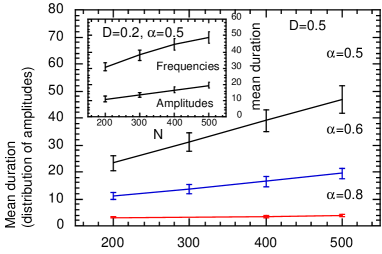
Figure 9: Mean durations $T_{S}$ until synchronization for the model with a distribution of amplitudes of width $l=0.5$ around the unit for $\alpha=0.5,0.6,0.8$(top to bottom) as a function of the population size $N$. Inset: mean durations to synchronization for the models with a distribution of amplitudes (bottom) and of frequencies (top) for a distribution width $D=0.2$ and $\alpha=0.5$. For the frequencies $T_{S}\simeq 19+0.06N$

As in the model with a distribution of frequencies, complete synchronization occurs independently of the initial values of the phases (states) if the locking conditions of all the oscillators in a single group are fulfilled. The conditions for this locking depend however on the models. Starting the evolution of the system from random phases, the formation of the possible stable groups comes from the evolution of the relative phase gaps between the oscillators due to different rhythms which have their origin in the quenched disorder on the characteristics of the oscillators. In the model with different slopes they come from the different phase advance responses to pulses of the oscillators.

For a given level of disorder and same $\alpha$ the probability of synchronization is much higher in the case of a disorder on the amplitudes (thresholds) than on the frequencies with also shorter $T_{S}$ (fig.9 inset). In short, disorder on the amplitudes and slopes is not a strong restriction of synchronization which is much more limited by the disorder on the frequencies. It is however not possible to conclude directly on what happens when both disorder exist simultaneously and we shall now therefore study this case.

3.3 Disorder on the frequencies and amplitudes

The mechanism of synchronization that we saw at work in systems with two different kinds of disorder is still at work and leads also to synchronization in a system with mixed disorder as well on the frequencies as on the thresholds. For two oscillators $O_{i}$ and $O_{j}$ as previously, the first return map for the phase of $O_{j}$ is now

$$\phi_{j}^{k+1}=\phi_{j}^{k}+\Delta_{i,j}$$ (13)

with

$$\Delta_{i,j}=(\phi_{j}^{c}-\phi_{i}^{c})+\frac{a_{j}-a_{i}}{a_{i}a_{j}}\delta$$ (14)

The phase variation $\Delta_{i,j}$ is due now as well to the difference of the free frequencies (first term of (14)) as to the different response of oscillators of different slopes to pulses (second term of (14)). Since there is no relation between the signs of $(\phi_{j}^{c}-\phi_{i}^{c})$ and of $({a_{j}-a_{i}})$ the two terms may be opposite. But generically they do not cancel each other since the periods and slopes are random. The phase gap between $O_{i}$ and $O_{j}$ varies therefore monotonically and both oscillators avalanche at some time together.

Here also there are locking conditions of oscillators in avalanches so that stable groups form and may grow up to complete synchronization. However it is not possible in this case to get the probability of complete synchronization proceeding as previously by simply establishing the locking conditions for all the $N$ oscillators in an avalanche. These conditions are necessary but not sufficient anymore to ensure synchronization for any initial distribution of the oscillator states. Indeed it is possible to verify that for large disorder there are cases were the formation of a stable group between two oscillators $O_{i}$ and $O_{j}$ with $a_{i}>a_{j}$ actually depends on the configuration of the phase values in the system and of its history (fig.10).

Figure 10: Oscillators with a spread of periods and thresholds $(\phi_{i}^{c},a_{i})\in[1-l/2,1+l/2]^{2}$. Two oscillators $O_{i}$ and $O_{j}$ with $\phi_{i}^{c}<\phi_{j}^{c}$ and $a_{i}>a_{j}$ have different locking conditions according to the strength of the dephasing pulse $\Delta$. The locking condition depends on the order of the firings which depends on $\Delta$. For a small$\Delta$, $O_{i}$ is at the threshold before $O_{j}$. For a large $\Delta$ (case represented in the figure), the oscillator $O_{j}$ which has the largest period is first at the threshold.

We studied the probability of synchronization numerically on simulations with random thresholds and periods uniformly distributed in $[1-D/2,1+D/2]*[1-D/2,1+D/2]$. We see on fig.11 for $N=300,400,500$ and $\alpha=0.5$ that up to $D\sim 0.1$ complete synchronization occurs in more than $99\%$ of the cases and that the probability is still high for larger widths.

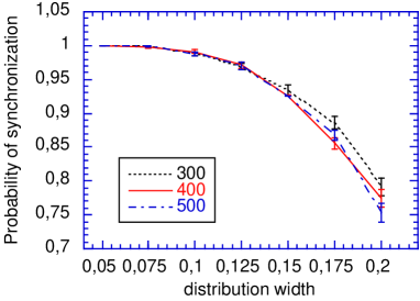
Figure 11: Probability of synchronization for a system of $N$ oscillators with a uniform spread of periods and thresholds $(\phi_{i}^{c},a_{i})\in[1-l/2,1+l/2]^{2}$, with $N=300,400$ as a function of the width $l$ for $\alpha=0.5$. Each point is the probability obtained with $1000$ samples of random oscillator parameter and is represented with the statistical error.

In the cases without complete synchronization the asymptotic behavior consists in the periodic avalanches of a large stable group with some few small ones. For small disorder the probability of synchronization depends only weakly on $N$: for a given $D$ the probabilities found for $N=300,400,500$ are all within the statistical errors.

As seen on fig. 12 the duration of the transient occurs in only a few periods although it increases polynomially with the disorder width. While the duration increases also with the population size $N$, we do not have enough data to establish a precise relation.

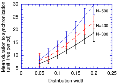
Figure 12: Mean duration $T_{S}$ until synchronization for the models with disorder on the frequencies and on the thresholds $(\phi_{i}^{c},a_{i})\in[1-l/2,1+l/2]^{2}$ as a function of the distribution width for $N=500,400,300$ and $\alpha=0.5$. $T_{S}$ grows polynomially with $D$, for $N=500$, $T_{S}\simeq 4.5+63D+316D^{2}$ with correlation coefficient $0.99992$.

At this point it is not difficult to imagine other models that synchronize following the same principles. A model with a distribution of frequencies and slopes and with constant threshold as been presented in [47]. We can also consider disorder on the pulse strengths. Let us, for instance, take a population of identical oscillators with a quenched disorder only on the pulse strengths so that the firing on an oscillators $O_{i}$ transmits to the rest of the system a pulse of strength $\alpha_{i}/N$. The phase gap between two oscillators $O_{i}$ and $O_{j}$ varies then as $s_{i,j}=(\alpha_{i}-\alpha_{j})/N$. Since generically the $s_{i,j}\neq 0$ any two oscillators participate at some time in the same avalanche and since the slopes and thresholds are identical the two oscillators are automatically locked.

We see finally that with instantaneous pulses, models with quenched disorder on several oscillator characteristics may also evolve to synchronization by the same mechanism of evolution of the gaps and locking in stable groups. The analysis and the estimation of the probability of synchronization is however more complicated.

4 Conclusion

In this article we have highlighted on some simple models the existence of several mechanisms leading to synchronization of IF oscillators. A surprising result is that contrary to a common belief, synchronization can actually occur even in basic models and for identical oscillators independently of the shape of the oscillators. In particular oscillators do not need to have a convex evolution function in order to synchronize. Therefore the common interpretation that “leakiness” in the evolution of the free oscillators, which implies convexity, is necessary for synchronization should be revised. We conclude that the observation of synchronization in a system of IF oscillators implies by itself nothing about the shape of the oscillator internal state variation function $E(\phi)$. Actually, for very concave oscillators synchronization occurs very easily for the natural choice of initial random phases. It is the opposite for a random initial distribution of the states. Therefore the nature of the random configuration at the beginning of the evolution has possibly important consequences. It would be interesting to study if the nature of the random initial configuration has similar consequences also in more sophisticated models.

In this article we assumed direct additivity of the pulses, which is probably an excessive requirement for realistic applications. The positive feedback effect between groups of different sizes, which is the only mechanism of synchronization for linear oscillators, occurs also for a softer form of additivity where the pulse from one group is not directly proportional to the number of oscillators in the group but merely an increasing function of it. Softer additivty would however increment the duration of the transient towards synchronization and reduce the range of favorable parameters in the case with disorder.

Concerning additivity we see that it is nevertheless true that convexity favors synchronization, since it is the only case which synchronizes also without additivity. However without additivity, i.e. without positive feedback, the duration of the transient diverges then at least as $(1-a)^{-1}$ in the linear limit $a\rightarrow 1$ [36]. Therefore without additivity a large convexity is necessary to keep the durations of the transitory not too long.

Let us mention that as shown recently by Tsodyks et al.[40], Hansel et al.[42] and Abbott and van Vreeswijk [41] smooth pulses with finite rise and fall time can crucially affect the behavior and destabilize synchronization. In this article we assume fast interactions and absorption: when two oscillators fire one after the other, the pulse of the second one occurs entirely during the refractory time of the first so that the oscillators synchronize in phase. The existence of a refractory time and absorption (i.e. assumption of fast pulses) is however not necessary for synchronization for identical convex and linear oscillators, in which case synchronization occurs also without absorption as locking of the oscillators in stable avalanches, in other words this corresponds to out-of-phase locking of the oscillators.

For identical linear and concave oscillators the probability of synchronization depends entirely on the initial configuration of the phases/states of the system. Indeed, some sets of initial configurations do not synchronize, for instance when the initial phases are equally spaced so that no group can be formed or in cases where the evolution leads to configurations with groups of the same size. For linear and highly concave $E(\phi)$ the measure of the unfavorable initial configuration is vanishingly small. It is larger and limits the probability of complete synchronization for “moderate” concavity. The degeneracy of the non favorable configuration disappears if some disorder is included in the models such as a small spread on the frequencies, thresholds or pulse strengths.

With fast pulse we found indeed that synchronization is possible also with a range of disorder on the oscillator characteristics. We find that the most difficult situation for synchronization is when the oscillators have different frequencies, where, for small disorder, a system with a given random sample of frequencies synchronizes almost always but, for larger disorder, the probability of synchronization decreases rapidly. Synchronization occurs then in the form of locking in avalanches and should be affected by softer additivity. On the other hand, disorder on the shape of the oscillators – occurring here through disorder on the thresholds and hence different slopes– with otherwise identical frequencies does not constraint severely synchronization. When both kinds of disorder are mixed the probability of complete synchronization is limited by the spread on the frequencies.

A point of interest would be to investigate how the discussed effects occur in more complex realistic models for instance of biological relevance. In particlar it would be important to study the robustness of the results when the interaction pulses have finite rise and fall times and for systems that are not globally coupled.

ACKNOWLEDGMENTS:
I am grateful to B. Delamotte for his helpful advice and supervision. I am also indebted to C. Pérez and A. Díaz-Guilera for fruitful discussions. Laboratoire de Physique Théorique et Hautes Energies is a Unité associée au CNRS: D 0280.

Appendix A APPENDIX A: PROOF OF SYNCHRONIZATION FOR SMALL CONCAVITY

In this appendix we prove the synchronization of an assembly of $N$ identical oscillators with state evolution function $E(t)=t^{a},t\in[0,1],a>1$ in the limit $a\rightarrow 1$. Let us first study the synchronization of only two isolated groups $G_{i}$ and $G_{j}$ of respectively $N_{i}$ and $N_{j}$ oscillators with $(N_{i}>N_{j})$ in absence of any other exterior pulses.

$$\mathbf{G_{i}}$$

at threshold

Relaxation of

at threshold

Relaxation of

at threshold

Table 5: Evolution of the phases of two isolated groups $G_{i}$ and $G_{j}$ of $N_{i}$ and $N_{j}$ oscillators $(N_{i}>Nj)$ on a cycle where the firing of the first group does not succeed to drag the second one along in an avalanche $((\phi_{j}^{k})^{a}+N_{i}\delta<E_{c}=1)$.

In table 5, we trace the variation of the phases and state variables of the two groups on a cycle of relaxations beginning with the largest group at the threshold. We deduce from there that the first return map for the phase of the second group $G_{j}$ is

$$\phi_{j}^{k+1}=1-\Big{(}1-\bigg{[}(\phi_{j}^{k})^{a}+N_{i}\delta\bigg{]}^{1\over a}+N_{j}\delta\Big{)}^{1\over a}.$$ (15)

which has an attractive fixed point $\phi_{0}(a,N_{i},N_{j},\delta)$. If the new phase after a cycle $\phi_{j}^{k+1}$ is in the interval $I_{c}\equiv[\phi_{c}(a,N_{i},\delta),1]$ where $\phi_{c}(a,N_{i},\delta)=(1-N_{i}\delta)^{1\over a}$ then $G_{j}$ is absorbed in the relaxation of $G_{i}$ (see fig.13).

Figure 13: Test for the synchronization of two groups for concave oscillators. a. The firing of $G_{1}$ causes the avalanche of the second group $G_{2}$ if $E_{2}+N_{1}\delta\geq 1$, that is if $\phi_{j}^{(k+1)}\geq\phi_{c}$. $\phi_{0}$ is the fixed point of the first return map for the phase of $G_{2}$ on each cycle beginning with $G_{1}$ at the threshold. b.) If $\phi_{j}^{(k+1)}<\phi_{c}$ the second groups never comes sufficiently close to the first one in order to avalanche together.d in the figure), the oscillator $O_{j}$ which has the largest period is first at the threshold.

$\phi_{c}$ corresponds to the phase at which $G_{j}$ is just pushed at the threshold by the pulse of $G_{i}$. If $\phi_{0}>\phi_{c}$, then the gap between the two groups gets smaller on each repeated cycle until it becomes sufficiently small for the groups to avalanche together and to merge. On the other hand if $\phi_{0}<\phi_{c}$ the two groups never avalanche together and remain apart. It is analytically difficult to test directly if $\phi_{0}$ is in $I_{c}$. However, since (15) is monotonic on each side of the fixed point, it is more convenient to test if $\phi_{j}^{k+1}$ is in $I_{c}$ when $\phi_{j}^{k}=\phi^{c}$, i.e. is just at the border of $I_{c}$. With $\phi_{j}^{k}=\phi_{c}$ this gives the inequality:

$$h(N_{i},N_{j})\equiv\phi_{j}^{k+1}-\phi_{j}^{k}=1-(1-N_{i}\delta)^{1\over a}-(N_{j}\delta)^{1\over a}\geq 0,$$ (16)

where $h(N_{i},N_{j})$ is the variation of the phase of $O_{j}$ on a cycle assuming $\phi_{j}^{k}=\phi_{c}$. Let us examine (16) for two groups with sizes $(N+c)/2$ and $(N-c)/2$. The function $g(c)\equiv h((N+c)/2,(N-c)/2)$ is monotonically increasing in $c$ so that the attraction between the two groups is stronger when the size difference is bigger. For a given $N$ and $a$ the condition $g(c)\geq 0$ is fulfilled when $c\geq\bar{c}(a,N)$ with

$$\bar{c}=\frac{N(1-a)}{2\alpha a}\left((1-\frac{\alpha}{2})\ln\left(1-\frac{\alpha}{2}\right)+\frac{\alpha}{2}\ln\left(\frac{\alpha}{2}\right)\right)+o\left((a-1)^{2}\right).$$ (17)

Contrary to the case of linear oscillators, two groups of different sizes – not only of equal size – may remain apart and not synchronize: if their size difference is too small, i.e. $c<\bar{c}$, positive feedback is not efficient enough and absorption does not occur. $\bar{c}(a,N)$ is an increasing function of $a$, so that for larger concavities less configurations with two groups can synchronize. We will see that this determines the probability that a system with $N$ random initial phases synchronizes.

Up to now we have considered only two isolated groups. In order to see if synchronization can occur when there are more groups, let us choose two groups and see if at some time they merge together. With many groups it is not possible to write a simple first return function on a cycle for the gap between two successive groups since this return map depends sensitively on the history of the system during this cycle. However we can simplify the question and prove that two groups can merge by focusing on the most severe condition. For that, let us isolate the two groups from the rest of the system as if they would not be affected by the pulses from the oscillators outside of the pair. It is easy to see that if the two groups can synchronize in these circumstances, they still synchronize in the real situation with the influence of exterior pulses. Indeed, the pulses of the rest of the system increment all the states in the same way and so they do not change the gap $E_{i}(t)-E_{j}(t)$. Therefore if $O_{i}$ and $O_{j}$ are close enough to avalanche together, they do so independently of pulses of other oscillators in the system. We can therefore focus our study on the case of an isolated pair of oscillators. Let the sizes of the two groups be $n$ and $n-c$. The groups merge if (18) is fulfilled with $N_{i}=n$ and $N_{j}=n-c$. Differently from previously we now study (16) with $N_{i}+N_{j}\neq N$. Since $h(n,n-c)$ is again a monotonically increasing function of $c$, the bigger is $c$, the stronger is the attraction. Therefore the most stringent condition for synchronization is for two groups of minimal size difference. Keeping this in mind we should now examine (16) as a function of $n$, i.e. we examine $f(n)\geq 0$ with $f(n)\equiv h(n,n-c)$ when $n\in[c+1,(N+c)/2]$. The function $f(n)$ is monotonically decreasing on the variation interval of $n$ with the highest value $f(c+1)\geq 0$. The smallest value $f(\frac{N+c}{2})$ is equal to $g(c)$. This value is the change in phase that we studied previously for a system of two groups of sizes $\frac{N+c}{2}$ and $\frac{N-c}{2}$. If the condition $g(c)\geq 0$ is fulfilled, then $f$ is also positive over the whole interval $n\in[c+1,(N+c)/2]$ and any pair of groups with size difference $c$ synchronizes. Finally we see that it is for the case of only two groups of sizes $\frac{N+c}{2}$ and $\frac{N-c}{2}$ that synchronization is the most difficult and it is this case that determines the most stringent condition for this phenomenon. Therefore, assuming that, as in the case of linear oscillators, synchronized pairs spontaneously form during the first cycle we find that the probability that the system synchronizes completely for random initial phases corresponds to the probability that $c<\bar{c}(a,N)$. Unfortunately this is also difficult to calculate. The system synchronizes with highest probability if synchronization is possible even for two groups of sizes $(N+1)/2$ and $(N-1)/2$, that is if $g(c=1)\geq 0$. This is the case when

$$a<\bar{a}\equiv 1-\frac{\alpha}{N}\left(\left((1-\frac{\alpha}{2}\right)\ln\left(1-\frac{\alpha}{2}\right)+\frac{\alpha}{2}\ln\left(\frac{\alpha}{2}\right)\right)^{-1}+o\left(\alpha\frac{1}{N^{2}}\right).$$ (18)

Since $\bar{a}>1$ there is an interval of concavities with the same conditions of synchronization than the linear case. Then synchronization can stop only if the two last groups are of the same size. Since $\bar{a}$ is close to $1$, the corresponding range of concave functions is quite small. However as discussed in 2.2, synchronization occurs in practice also with high probability for much larger concavities.

Appendix B APPENDIX B: DISTRIBUTION OF AMPLITUDES

In this appendix we detail the conditions under which synchronization occurs in the model of section (3.2) of oscillators with a distribution of amplitudes (thresholds). We follow the same steps as for the model with a distribution of frequencies (3.1).

$$\mathbf{\phi_{i}}$$

a.

b.

c.

d.

d.

Table 6: a. $O_{i}$ at the threshold; b. Firing of $O_{i}$ , $O_{j}$ received a pulse $\delta$ causing an advance in phase $\delta/a_{j}$; c. $O_{j}$ at the threshold, the term $(j-2)\delta\frac{a_{j}-a_{i}}{a_{j}a_{i}}$ comes from the $(j-2)$ other pulses since the relaxation of $O_{i}$; d. Firing of $O_{j}$; e. $O_{i}$ back at the threshold; $(N-j+1)$ other pulses from the rest of the system occurred since the relaxation of $O_{i}$.

From table 6 we get the first return map for the phase of $O_{j}$ on a cycle beginning with $O_{i}$ at the threshold:

$$\phi_{j}^{(k+1)}=\phi_{j}^{(k)}+(N-1)\delta\frac{a_{j}-a_{i}}{a_{j}a_{i}}.$$ (19)

Let $a_{j}>a_{i}$, then on each cycle $\phi_{j}$ is closer to $\phi^{c}=1$. The phase difference $\phi_{i}-\phi_{j}$ decreases and after some repetitions of the cycle the firing of $O_{i}$ drags $O_{j}$ along in an avalanche. Therefore as in section 3.1 also in this model any two oscillators avalanche at some time together. The change in the phase gaps between the oscillators that finally cause the simultaneous firings has for origin the different rhythms of firings of the oscillators. Contrary to the previous model where the different rhythms were intrinsic, now the different rhythms of firings of the oscillators are only effective and caused by the different responses of the oscillators to pulses. Indeed the value of the phase advance caused by a pulse of given strength depends on the slopes of the oscillators. Due to the quenched disorder on the slopes the oscillator evolve more or less rapidly under the phase advance caused by pulses and have therefore different effective rhythms of evolution. The evolution towards synchronization due to the different rhythms comes in addition to the positive feedback attraction between groups of different sizes which causes also the evolution of the phase gaps between oscillators. Both effects drive the system in the state of maximal synchronization compatible with the disorder.

We establish now the stability conditions of synchronized groups, i.e. the conditions of locking in avalanches. Two oscillators $O_{i}$ and $O_{j}$, say with $a_{j}>a_{i}$ that avalanche together and are in phase at the origin $\phi_{i}=\phi_{j}=0$ are dephased by the pulses from other oscillators, the oscillator $O_{i}$ with the smallest slope being the most advanced. Let $\Delta$ be the summed strength of the pulses of the other oscillators between the last simultaneous avalanche of $O_{i}$ and $O_{j}$ and the return of $O_{i}$ back at the threshold. $\Delta$ shifts the two oscillators apart by the phase difference $\tau=\Delta(a_{i}-a_{j})/(a_{i}a_{j})$. If the slopes $a_{i}$ and $a_{j}$ are close enough then $\tau$ is sufficiently small for $O_{i}$ and $O_{j}$ still to relax in the same avalanche triggered by $O_{i}$. The locking condition for two oscillators that avalanched together is (see fig. 8):

$$\Delta\frac{a_{i}-a_{j}}{a_{i}a_{j}}<\frac{\delta}{a_{j}}.$$ (20)

If $O_{i}$ and $O_{j}$ were the only oscillators in their avalanche then $\Delta=(N-2)\delta$ and (20) is equivalent to ${a_{i}-a_{j}}<a_{i}/(N-2)$.

For a group of $m\geq 2$ oscillators $O_{i},i=1\dots m$ with $a_{i+1}>a_{i}$ the locking conditions are:

$$(a_{i}-a_{1})<a_{1}\frac{i-1}{N-m}\ \ \ ,\ \ \ i=1\dots m.$$ (21)

These inequalities are obtained considering that

1. the $m$ oscillators that avalanched together and were at the origin are dephased by a total pulse $\Delta=(N-m)\delta$ before the oscillators $O_{1}$ is back, the first of them, at the threshold.

2. the $i$-th oscillator in the avalanche receives $i-1$ pulses from the oscillators that preceded it.

Complete synchronization is possible if (21) is fulfilled for $m=N-1$. Indeed, if this is the case a stable group with $N-1$ elements forms. Then, this group and the last $N$-th oscillator of the system inevitably participate in a same avalanche and the whole system becomes in phase without, now, any exterior dephasing pulse.

The relation (12) in section 3.2 gives the probability for a uniform random distribution of $N$ slopes in an interval $[a-\frac{D}{2},a+\frac{D}{2}]$ of fulfilling (21).

References

- [*] e-mail address: bottani@lpthe.jussieu.fr
- [1] R. Roy and K. Thornburg, Phys. Rev. Lett. 72, 2009 (1994).
- [2] D. Fisher, Phys. Rev. B 31, 1396 (1985).
- [3] S. Strogatz, C. Marcus, R. Westervelt, and R. Mirollo, Physica D 36, 23 (1989).
- [4] P. Hadley, M. Beasley, and K. Wiesenfeld, Phys. Rev. B 38, 8712 (1988).
- [5] R. Mirollo, S. Strogatz, and K. Wiesenfeld, Physica D 48, 102 (1991).
- [6] Y. Kuramoto, Chemical Oscillation Waves and Turbulence (Springer, Berlin, 1984).
- [7] J. Neu, SIAM J. Appl. Math. 38, 305 (1980).
- [8] A. Winfree, J. Theor. Biol. 16, 15 (1967).
- [9] J. Buck, Quart. Rev. Biol. 63, 265 (1988).
- [10] J. Buck and E. Buck, Scientific American 234, 74 (1988).
- [11] F. Hanson, F. Case, J. Buck, and E. Buck, Science 174, 161 (1971).
- [12] G. Ermentrout, J. Math. Biol. 29, 571 (1991).
- [13] S. Strogatz, Lecture Notes in Biomathematics 100, (1993).
- [14] E. Sismondo, Science 249, 55 (1990).
- [15] T. Walker, Science 166, 891 (1969).
- [16] J. Hopfield, Nature 376, 33 (1995).
- [17] W. Gerstner, Phys. Rev. E 51, 738 (1995).
- [18] Y. Kuramoto, J. Stat. Phys. 49, 569 (1987).
- [19] Y. Kuramoto, Prog. of Theor. Phys. 79, 223 (1984).
- [20] H. Daido, Prog. of Theor. Phys. 77, 622 (1987).
- [21] H. Daido, Phys. Rev. Lett. 61, 231 (1988).
- [22] H. Sakaguchi, S. Shinomoto, and Y. Kuramoto, Prog. of Theor. Phys. 77, 1005 (1987).
- [23] S. Strogatz and R. Mirollo, J. Phys. A 21, L699 (1987).
- [24] Y. Yamaguchi and H. Shimizu, Physica D 11, 212 (1984).
- [25] M. Shiino and M. Frankowicz, Phys. Lett. A 136, 103 (1986).
- [26] P. Matthews and S. Strogatz, Phys. Rev. Lett. 65, 1701 (1990).
- [27] G. Ermentrout, Physica D 41, 219 (1990).
- [28] D. Hansel, G. Mato, and C. Meunier, Phys. Rev. E 48, ?? (1993).
- [29] D. Hansel, G. Mato, and C. Meunier, Europhys. Lett. 23, 365 (1993).
- [30] D. Hansel, G. Mato, and C. Meunier, Concepts in Neuroscience 4, 193 (1993).
- [31] P. Matthews, R. Mirollo, and S. Strogatz, Physica D 52, 1293 (1991).
- [32] L. Lapique, J. Physiol. Pathol. Gen. 9, 620 (1907).
- [33] L. Glass and M. Mackey, From Clocks to chaos:The Rhytms of Life (Princeton university Press, Princeton, NJ, 1988).
- [34] H. Smith, Science 82, 151 (1935).
- [35] C. Peskin, Mathematical Aspects of Heart Physiology, Courant Inst. of Math. Sci. Publication, 1975.
- [36] R. Mirollo and S. Strogatz, SIAM J. Appl. Math. 50, 1645 (1990).
- [37] Y. Kuramoto, Physica D 50, 15 (1991).
- [38] A. Corral, C. Pérez, A. Dí az Guilera, and A. Arenas, Phys. Rev. Lett. 75, 3697 (1985).
- [39] U. Ernst, K. Pawelzik, and T. Geisel, Phys. Rev. Lett. 74, 1570 (1995).
- [40] M. Tsodyks, I. Mitkov, and H. Sompolinsky, Phys. Rev. Lett. 71, 1280 (1993).
- [41] L. Abbott and C. van Vreeswijk, Phys. Rev. E 48, 1483 (1993).
- [42] D. Hansel, G. Mato, and C. Meunier, Neural Computation 7, 307 (1995).
- [43] W. Gerstner and J. van Hemmen, Phys. Rev. Lett. 71, 1280 (1993).
- [44] D. Perkel, Biophys. J. 7, 391 (1967).
- [45] R. Stein, Biophys. J. 7, 797 (1967).
- [46] D. Cox, Renewal Theory (Methuen, London, 1962).
- [47] S. Bottani, Phys. Rev. Lett. 74, 4189 (1995).
- [48] P. Bak, C. Tang, and K. Wiesenfeld, Phys. Rev. Lett. 59, 381 (1988).
- [49] D. Dhar, Phys. Rev. Lett. 64, 1913 (1990).
- [50] Y. Zhang, Phys. Rev. Lett. 63, 470 (1989).
- [51] L. Kadanoff, S. Nagel, L. Wu, and S. Zhou, Phys. Rev A 39, 6524 (1989).
- [52] K. Sneppen, Phys. Rev. Lett. 69, 3539 (1992).
- [53] P. Bak and K. Sneppen, Phys. Rev. Lett. 71-75, 4083 (1993).
- [54] B. Drossel and F. Schwabl, Phys. Rev. Lett. 69-73, 1629 (1992).
- [55] K. Christensen, Ph.D. thesis, University of Aarhus, Denmark, 1992, p.49.
- [56] Z. Olami, H. Feder, and K. Christensen, Phys. Rev. Lett. 68, 1244 (1992).
- [57] A. Middleton and T. Tang, Phys. Rev. Lett. 74, 742 (1995).
- [58] A. Corral, C. Pérez, A. Dí az Guilera, and A. Arenas, Phys. Rev. Lett. 74, 118 (1995).
- [59] J. Herz, A.V.M. Hopfield, Phys. Rev. Lett. 75, 1222 (1995).
- [60] A. Winfree, The geometry of biological time (Springer, New York, 1980).
- [61] S. Bottani and D. Delamotte, 1994, (submitted).