DYNAMIC CONDUCTANCE IN QUANTUM HALL SYSTEMS

Abstract

In the framework of the edge-channel picture and the scattering approach to conduction, we discuss the low frequency admittance of quantized Hall samples up to second order in frequency. The first-order term gives the leading order phase-shift between current and voltage and is associated with the displacement current. It is determined by the emittance which is a capacitance in a capacitive arrangement of edge channels but which is inductive-like if edge channels predominate which transmit charge between different reservoirs. The second-order term is associated with the charge relaxation. We apply our results to a Corbino disc and to two- and four-terminal quantum Hall bars, and we discuss the symmetry properties of the current response. In particular, we calculate the longitudinal resistance and the Hall resistance as a function of frequency.

1 Introduction

In this work we discuss the low frequency response of two-dimensional conductors subject to a perpendicular quantizing magnetic field[1] and subject to time-dependent oscillating voltages applied to the contacts of the sample. We use an approach[2]${}^{\!-\,}$[4] closely related to the scattering approach to dc conduction[5] in a mesoscopic phase-coherent multiterminal sample. The approach treats current and voltage contacts on equal footing and views the entire sample and the nearby conductors as one electric entity.
It is well-known from mesoscopic conduction theory that all dc resistances are rational functions of transmission probabilities for carriers to reach a contact if they are injected at another contact.[5] Moreover, only the states at the Fermi surface which connect different contacts count. In a conductor subject to a quantizing magnetic field the only states at a Hall plateau which provide such a connection are the edge states which are the quantum mechanical generalization of the semi-classical ‘skipping orbits’ of the charge carriers along the sample boundary. As a consequence the dc conductance is quantized and determined by the topology of the edge-state arrangement.[5] For a lucid discussion of the current patterns and Hall potentials in the presence of transport, we refer the reader to a recent work by Komiyama and Hirai.[6]
Most of the early work on edge states relies on a picture valid for noninteracting electrons which must be modified in very pure samples with smooth boundaries.[7] Interaction leads to a decomposition of the electron gas into compressible and incompressible regions, where the former ones are associated with the edge states. Interaction must also be considered to describe edge states in the fractional quantum-Hall regime.[8] A detailed description of the contacts for chiral edge-state models has recently been provided by Kane and Fisher.[9] While in these works the main concern is with short-range interactions, we emphasize in our work the long-range part of the Coulomb interaction. For this case, edge states are important since they contribute to screening, in contrast to the bulk states.[6, 10] Due to the Coulomb interaction, the ac response is not only determined by the topology of the edge-state arrangement but also by its geometry.
In the following, we concentrate on a two-dimensional electron gas with spin-split Landau levels. Coulomb interaction is taken into account by consideration of the capacitances of all edge channels and all gates. We assume that additional contributions due to parasitic capacitances associated with contacts can be neglected, that the contacts are quantized, and that inter-edge scattering is absent.

2 Low-frequency admittance

2.1 Current conserving and gauge-invariant electric transport

The gates together with the edge channels which are separated by regions of incompressible electron gas can be seen as an arrangement of mesoscopic conductors embedded in a dielectric medium. We describe an $N$-terminal sample at a Hall plateau by an arrangement of such conductors $j=1,...,M$ connected to contacts $\alpha=1,...,N$ (see, e.g., Fig. 1). We are interested in the dynamical conductance $G_{\alpha\beta}(\omega)$ which determines the Fourier amplitudes of the current, $\delta I_{\alpha}$, at a contact $\alpha$ in response to an oscillating voltage $\delta V_{\beta}\exp(-i\omega t)$ at contact $\beta$

$$\delta I_{\alpha}=\sum_{\beta}G_{\alpha\beta}(\omega)\;\delta V_{\beta}\;\;.$$ (1)

The voltage variation $\delta V_{\beta}$ is related to the variation of the electro-chemical potential $\delta\mu_{\beta}$ in reservoir $\beta$ by $\delta\mu_{\beta}=e\delta V_{\beta}$, where $e$ is the electron charge.
Since all the present gates and conductors are included in the description, and due to the long-range nature of the Coulomb interaction the theory for the conductance has to satisfy two basic requirements, namely current conservation and gauge invariance. Current conservation corresponds to zero total current, $\sum_{\alpha}\delta I_{\alpha}=0$. Hence the total charge is conserved. Gauge invariance means that a global voltage shift, $\delta V_{\alpha}\mapsto\delta V_{\alpha}+\delta V$, does not affect the currents. In particular, we fix the voltage scale such that $\delta V_{\alpha}\equiv 0$ corresponds to the equilibrium state where all electrochemical potentials $\mu_{\alpha}$ are equal. Current conservation and gauge invariance demand the admittance matrix $G_{\alpha\beta}$ to satisfy $\sum_{\alpha}G_{\alpha\beta}=\sum_{\beta}G_{\alpha\beta}=0$. For example, the admittance of a two-terminal device is determined by a single scalar quantity, $G_{\alpha\beta}=(-1)^{\alpha+\beta}G$. Due to microreversibility the linear response coefficients must additionally satisfy the Onsager-Casimir reciprocity relations $G_{\alpha\beta}|_{B}=G_{\beta\alpha}|_{-B}$ where $B$ is the magnetic field. We are interested in the low-frequency limit and write

$$G_{\alpha\beta}(\omega)=G_{\alpha\beta}^{(0)}-i\omega E_{\alpha\beta}+\omega^{2}K_{\alpha\beta}+{\cal O}(\omega^{3})\;\;.$$ (2)

While the theory for the dc-conductances $G_{\alpha\beta}^{(0)}$ of quantized Hall systems is well established,[5] the emittance matrix $E_{\alpha\beta}\equiv i(dG_{\alpha\beta}/d\omega)_{\omega=0}$ has been investigated only recently.[2] Below we recall these results and, in addition, provide new results for the second order term $K_{\alpha\beta}\equiv(1/2)\>(d^{2}G_{\alpha\beta}/d\omega^{2})_{\omega=0}$. To get some feeling for the emittance and the second order term, consider a two-terminal device with a macroscopic capacitor $C$ in series with a resistor $R$. For this purely capacitive structure with zero dc-conductance one finds that the emittance is the capacitance, $E=C$, and that $K=RC^{2}$ contains the $RC$ time constant associated with charge relaxation. These simple results must be modified for mesoscopic conductors and conductors which connect different reservoirs.[3] Firstly, it is not the geometrical capacitance but rather the electro-chemical capacitance which relates charges on mesoscopic conductors to voltage variations in the reservoirs. Secondly, conductors which connect different reservoirs allow a transmission of charge which leads to inductance-like contributions to the emittance.

2.2 Transmission properties of edge channels

An important property of a single edge channel is its uni-directional transparency and the absence of backscattering.[5] The scattering matrix $s_{\alpha\beta}$ relates the out-going current amplitude at contact $\alpha$ to the incoming current amplitude at contact $\beta$. The part of the scattering matrix associated with edge channel $j$ can be written in the form $s_{\alpha\beta}^{(j)}=\Delta_{\alpha j}t_{j}\Delta_{j\beta}$ with a scattering amplitude $t_{j}=\exp(i\phi_{j}(E))$. The energy dependence of the phase $\phi_{j}(E)$ determines the density of states of the edge channel, $dN_{j}/dE=(1/2\pi)(d\phi_{j}/dE)$ at the Fermi energy. We mention that for noninteracting particles the density of states is related to the electric field at the edge.[5] $\Delta_{j\alpha}$ and $\Delta_{\alpha j}$ are the injection and emission probability, respectively, of channel $j$ at contact $\alpha$:

$$\Delta_{j\alpha} = \cases{1&${\rm if\;contact}\;\;\alpha{\rm\;\;injects\;into\;channel\;\;}j$\cr 0&$\;\;\;\;{\rm otherwise}$\cr}$$ (3)

$$\Delta_{\alpha j} = \cases{1&${\rm if\;channel}\;\;j{\rm\;\;emits\;into\;contact\;\;}\alpha$\cr 0&$\;\;\;\;{\rm otherwise}$\cr}\;\;.$$ (4)

Since an edge channel is always connected to one contact at each of its ends, one has $\sum_{\alpha}\Delta_{k\alpha}=\sum_{\alpha}\Delta_{\alpha k}=1$. Furthermore, $\sum_{k}\Delta_{k\alpha}$ ($=\sum_{k}\Delta_{\alpha k}$) is the number of edge channels which enter (leave) the sample at contact $\alpha$. Clearly, the transmission probabilities are functions of the magnetic field $B$ and obey the micro-reversibility conditions $\Delta_{\alpha k}(B)=\Delta_{k\alpha}(-B)$. This follows directly from the fact that an inversion of the magnetic field inverses the arrows attached to the edge states. In terms of the $\Delta_{j\alpha}$ and $\Delta_{\alpha j}$ the dc conductance becomes[2]

$$G_{\alpha\beta}^{(0)}=\frac{e^{2}}{h}\sum_{k}\biggl{(}\Delta_{k\alpha}\>\Delta_{k\beta}-\Delta_{\alpha k}\Delta_{k\beta}\biggr{)}\;\;.$$ (5)

Hence the topology of the edge-channel arrangement determines the dc conductance. Note that current conservation, gauge invariance, and the Onsager-Casimir relations follow immediately from the properties of $\Delta_{j\alpha}$ and $\Delta_{\alpha j}$.

2.3 Screening properties: a discrete model

While the dc-conductance is completely determined by the overall transmission, the ac-conductance contains information on the nonequilibrium state within the sample. Application of an oscillatory voltage at a sample contact leads to a periodic charging of the sample, and the induced electric fields have to be taken into account self-consistently. In order to treat the dynamic charge and potential distribution in the nonequilibrium state we spatially discretize the two-dimensional electron gas. More concrete, we assign to each edge channel $j$ a single electrochemical potential of the carriers, a single electrical potential, and a total charge. We neglect spatio-temporal effects inside edge channels such as edge plasmons with finite wave numbers.[11, 12] However, our discussion takes into account the zero wave-number modes of the edge states. The electrochemical potential shift $\delta V_{j}$ in edge channel $j$ can be written in terms of the voltages $\delta V_{\beta}$ in the reservoirs, $\delta V_{j}=\sum_{\beta}\Delta_{j\beta}\>\delta V_{\beta}$. To simplify notation we write quantities associated with edge channels as $M$-dimensional vectors, e.g. ${\bf\delta V}=(\delta V_{1},...,\delta V_{M})^{t}$. The nonequilibrium distribution of charges and electric potentials ${\bf\delta q}=(\delta q_{1},...,\delta q_{M})^{t}$ and ${\bf\delta U}=(\delta U_{1},...,\delta U_{M})^{t}$, respectively, are related by ${\bf\delta q}={\bf C\>\delta U}$, where ${\bf C}$ is the geometrical capacitance matrix for the edge channels and gates. As usual, ${\bf C}$ can be obtained from the Poisson equation. A relation between the charges and the voltages of the reservoirs, ${\bf\delta q}={\bf C_{\mu}\;\delta V}$, defines the electrochemical capacitance matrix ${\bf C_{\mu}}$. Note that while ${\bf C}$ is real and frequency independent, ${\bf C_{\mu}}(\omega)$ is a function of frequency. Here, we define ${\bf C}$ by assuming that each edge channel is connected to its own reservoir, hence charge conservation and gauge invariance imply for both ${\bf C}$ and ${\bf C}_{\mu}(\omega)$ the sum rules $\sum_{k}C_{kl}=\sum_{l}C_{kl}=\sum_{k}C_{\mu,kl}=\sum_{l}C_{\mu,kl}=0$. Both matrices are symmetric and even functions of the magnetic field. Further we need the dynamic densities of states of the edge channels. In the present notation they can be summarized in a diagonal matrix ${\bf D}(\omega)$ with elements $D_{jj}(\omega)=e^{2}(dN_{j}/dE)(1+i\tau_{j}\omega/2)+{\cal O}(\omega^{2})$.[13] Here, $\tau_{j}=h(dN_{j}/dE)$ is the dwell time of carriers in edge channel $j$. The specific form of the $D_{jj}(\omega)$ can be understood by noticing that the charging of edge channel $j$ is a relaxation process with a time $\tau_{j}/2$. The nonequilibrium charge is ${\bf\delta q}={\bf D}({\bf\delta V}-{\bf\delta U})={\bf C\delta U}={\bf C}_{\mu}{\bf\delta V}$ from which one obtains the dynamic electrochemical capacitance

$${\bf C}_{\mu}(\omega)={\bf C}_{\mu}(0)+i\omega\frac{h}{2e^{2}}{\bf C}_{\mu}^{2}(0)+{\cal O}(\omega^{2})\;\;,$$ (6)

where ${\bf C}_{\mu}(0)=[{\bf 1}+{\bf CD}^{-1}(0)]^{-1}{\bf C}$ is the static part of the electrochemical capacitance matrix. The dependence of the effective capacitance ${\bf C}_{\mu}(0)$ on the densities of states is reasonable: small densities of states make it more difficult to charge the conductor. For large densities of states, on the other hand, one recovers the geometrical capacitance.

2.4 The dynamic response

The low frequency admittance can be calculated with the help of a recent theory which generalizes the scattering approach to ac conduction.[4] The ingredients which we need are the current response to an external voltage shift $\delta{\bf V}$ and the current response to an internal voltage shift $\delta{\bf U}$ for carriers at the Fermi energy $E_{F}$ and for carriers with energies $E_{F}+\hbar\omega$. We do not enter into details here but present only the result. We find

$$G_{\alpha\beta}(\omega)=G_{\alpha\beta}^{(0)}-i\omega\sum_{k,l=1}^{N}\Delta_{\alpha k}\>C_{\mu,kl}(\omega)\>\Delta_{l\beta}\;\;.$$ (7)

Using the micro-reversibility properties of the $\Delta_{\alpha k}$ and the symmetry of the capacitance matrix it is again easy to prove current conservation, gauge invariance, and the Onsager-Casimir reciprocity relations. The results (6) and (7) yield the admittance to order ${\cal O}(\omega^{2})$. The emittance $E_{\alpha\beta}=\sum_{kl}\Delta_{\alpha k}$ $C_{\mu,kl}(0)\Delta_{l\beta}$ can be understood as the sum of all ‘two-body’ Coulomb interactions between edge states and/or gates.[2] In a pure capacitive arrangement where $\Delta_{k\alpha}=\Delta_{\alpha k}$ the emittance matrix is a capacitance matrix, i.e. diagonal elements are positive and off-diagonal elements are negative. As we will see below, this can change in the presence of edge channels which connect different reservoirs. The result for the second-order term, $K_{\alpha\beta}=(h/2e^{2})$ $\sum_{kjl}\Delta_{\alpha k}C_{\mu,kj}(0)$ $C_{\mu,jl}(0)\Delta_{l\beta}$, can thus similarly be interpreted as a ‘three-body’ interaction with an intermediate step via edge channel (or gate) $j$. This simple result, of course, relies on the discrete model and is modified as soon as one includes internal spatio-temporal edge excitations.

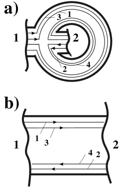
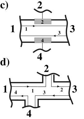
Figure 1: Two-terminal samples: a) Corbino disc and b) quantum Hall bar. Four-terminal samples: c) two-terminal Hall bar with two additional gates; d) four-terminal Hall bar

3 Examples

3.1 Two-terminal devices

Let us discuss the Corbino disc and the quantum Hall bar with $m$ channels along an edge as shown in Fig. 1 for a magnetic field $B$ such that $m=2$. Channels at the upper and the lower edges are labeled by odd and even numbers, respectively. Equation (6) permits now to treat the case where different edge states are at different potentials. For the sake of clarity, however, we assume that the capacitances between edge channels at the same edge are very large such that they are at equal potentials. We take thus each set together to form a single $m$-channel conductor associated with only even or only odd labels. The geometric capacitance between the two sets of channels is denoted by $C$ ($=\sum_{kl}C_{2k\>2l}$). While for the disc the reservoirs are capacitively coupled, for the bar all edge channels transmit charge between different reservoirs. Hence, the dc-conductance of the disc and the bar are $G(0)=0$ and $G(0)=me^{2}/h$, respectively. The dynamic capacitance between the two sets of edge channels is $C_{\mu}(\omega)=C_{\mu}(0)+i\omega RC_{\mu}^{2}$ with a static electrochemical capacitance given by $1/C_{\mu}(0)=1/C+(\sum_{{\rm even}}D_{i})^{-1}+(\sum_{{\rm odd}}D_{i})^{-1}$. The charge relaxation resistance is given by

$$R=\frac{h}{2e^{2}}\left(\frac{\sum_{i={\rm odd}}D_{i}^{2}}{(\sum_{i={\rm odd}}D_{i})^{2}}+\frac{\sum_{i={\rm even}}D_{i}^{2}}{(\sum_{i={\rm even}}D_{i})^{2}}\right)\;\;.$$ (8)

Due to the purely capacitive coupling the low frequency admittance of the Corbino disc is

$$G(\omega)=-i\omega C_{\mu}(\omega)=-i\omega C_{\mu}(0)+\omega^{2}RC_{\mu}^{2}(0)\;\;.$$ (9)

As one expects, this result is equivalent to the low frequency admittance of a mesoscopic capacitor with $m$ channels on each side.[4] On the other hand, one finds for the bar

$$G(\omega)=m\frac{e^{2}}{h}+i\omega C_{\mu}(\omega)=m\frac{e^{2}}{h}+i\omega C_{\mu}(0)-\omega^{2}RC_{\mu}^{2}(0)$$ (10)

While the emittance of the disc behaves like a capacitance, the emittance of the bar is inductive-like. Inductive behavior is a typical property of conductors where transmission between different reservoirs dominates.[3] The crossover between the two limits of a purely transmitting and a purely capacitive arrangement can be investigated by considering tunneling between edge channels. In a recent work, [14] we have shown that the emittance of a quantum point contact without magnetic field exhibits a change of the sign as a function of the transparency.
Note that if all $D_{j}$ are of the same order of magnitude, the charge relaxation resistance $R$ scales like $1/m$. Nevertheless, if $C_{\mu}$ scales with $m$ (as is the case on a Hall plateau and for large $C$) one has $G(\omega)\propto m$. At a transition between two Hall plateaus, however, the density of states of the innermost edge channel diverges and one expects the charge relaxation resistance to be of the order of a single resistance quantum.

3.2 Four-terminal devices

Figure 1c. shows a two-terminal bar with two additional symmetric gates each located close to an edge state. Macroscopic gates have huge densities of states which means that $C/D_{2}=C/D_{4}=0$, where $C=|C_{12}|=|C_{34}|$ is the geometric capacitance between a gate and the nearest edge channel. Note that the off-diagonal elements of the capacitance matrix are negative. We assume that the other off-diagonal capacitance elements are much smaller, i.e. $|C_{24}|=C_{g}\ll C$ and $C_{13}=C_{14}=0$. Now, let us ask for the current through contact $1$ in response to a voltage oscillation at gate $2$. We find to leading order of $C_{g}$ for the associated admittance $G_{12}|_{B}=\omega^{2}(h/2e^{2})C_{g}C_{3}+{\cal O}(\omega^{3})$ with $C_{3}=1/(C^{-1}+D_{3}^{-1})$. Clearly, since edge channel $3$ emits into reservoir $1$, and gate $2$ interacts only via gate $4$ with this edge channel, the response is proportional to $C_{g}C_{3}$ and of second order in frequency. On the other hand, by inverting the magnetic field, edge channel $1$ emits into reservoir $1$. Now, the relevant capacitance turns out to be $C_{1}=1/(C^{-1}+D_{1}^{-1})$; to leading order of $C_{g}$ we find $G_{12}|_{-B}=i\omega C_{1}+\omega^{2}(h/e^{2})C_{1}^{2}+{\cal O}(\omega^{3})$. Thus while $G_{12}|_{-B}$ exhibits a capacitive response given by $C_{1}$, the capacitive response in $G_{12}|_{B}$ is absent. Such a dramatic magnetic field asymmetry has been verified in an experiment by Chen et al. [15] in the absence of gate $4$, i.e. for $C_{g}=0$.
The result (7) implies that the conductance $G_{\alpha\beta}$ between two contacts which are capacitively coupled to the sample is a symmetric function of the magnetic field. This is in general true up to ${\cal O}(\omega)$.[3] To higher order in frequency, however, the magnetic-field symmetry of the current response can change in the presence of voltage probes. As an example, we assume $C_{g}=0$ and that contact $3$ in Fig. 1c. acts as a voltage probe. Using $\delta I_{3}=0$, we eliminate $\delta V_{3}$ from the Eqs. (1) and obtain the reduced admittance matrix $\tilde{G}_{\alpha\beta}$ associated with the contacts $1$, $2$, and $4$. We find $\tilde{G}_{24}|_{B}=0$ and $\tilde{G}_{42}|_{B}=\tilde{G}_{24}|_{-B}=\omega^{2}(h/e^{2})C^{2}$. Hence, the impedance of a purely capacitive arrangement is in general not symmetric but only governed by the Onsager-Casimir symmetry relations, $G_{\alpha\beta}|_{B}=G_{\beta\alpha}|_{-B}$. This conclusion has been drawn by Sommerfeld et al.[12] who found an asymmetric capacitance of a three-terminal Corbino disc. Our theory predicts such an asymmetric behavior in a simple way.
Another interesting question concerns the Hall resistance $R_{H}=(\delta V_{2}-\delta V_{4})/\delta I_{1}$ of the sample shown in Fig. 1c. If $C_{g}$ vanishes one expects exact quantization because the gates do nothing but measure the edge potentials. An expansion to first order in $C_{g}$ yields the low frequency resistance

$$R_{H} = \frac{h}{e^{2}}\>(1-C_{g}(C_{1}^{-1}+C_{3}^{-1}))$$ (11)

$$+ \frac{1}{2}\omega^{2}\frac{h^{3}}{e^{6}}\;\frac{C_{g}(C_{1}^{-1}+C_{3}^{-1})}{D_{1}^{-1}D_{3}^{-1}+C^{-1}(C^{-1}+D_{1}^{-1}+D_{3}^{-1})}+{\cal O}(\omega^{3})$$

In the case where the two gates are decoupled, one concludes indeed that the resistance is quantized, $R_{H}(\omega)=h/e^{2}$. However, due to the Coulomb coupling between the gates this result is modified even for the dc case.

The integer quantum Hall effect[1] corresponds to the quantization of the Hall resistance and the vanishing of the longitudinal resistance of the ideal four-probe quantum Hall bar of Fig. 1d. at zero frequency. Two of the contacts serve as voltage probes, whereas the two remaining contacts are used as source and sink for the current. With the help of our theory the dc-results can be extended to the low-frequency case. If the contacts $3$ and $4$ are the voltage probes, the longitudinal resistance is defined by $R_{L}=(\delta V_{4}-\delta V_{3})/\delta I_{1}$. The Hall resistance is defined by $R_{H}=(\delta V_{2}-\delta V_{4})/\delta I_{1}$, provided the contacts $2$ and $4$ are voltage probes. Let us assume that the elements $C_{\mu,kl}$ of the electrochemical capacitance matrix are known. For the specific geometry of Fig. 1d. we assume $C_{\mu,12}=C_{\mu,24}=C_{\mu,34}=0$ and calculate the low frequency admittance. From Eqs. (1), (6), and (7) we find then the longitudinal resistance

$$R_{L}=i\omega\>\frac{h^{2}}{e^{4}}C_{\mu,13}+\frac{\omega^{2}}{2}\frac{h^{3}}{e^{6}}C_{\mu,13}(C_{\mu,23}-C_{\mu,14})\;\;.$$ (12)

The leading term of the longitudinal resistance is determined by the Coulomb coupling between the current circuit and the voltage circuit which are represented by edge channels $1$ and $3$, respectively. This is even true for finite $C_{\mu,24}$.[2] Moreover, for the specific symmetry $C_{\mu,23}=C_{\mu,14}$ the dissipation vanishes also in ${\cal O}(\omega^{2})$. For the Hall resistance one finds

$$R_{H}=\frac{h}{e^{2}}-i\omega\>\frac{h^{2}}{e^{4}}C_{\mu,13}+\frac{\omega^{2}}{2}\frac{h^{3}}{e^{6}}C_{\mu,13}(C_{\mu,23}+C_{\mu,14})\;\;.$$ (13)

We mention, that if we had chosen the symmetry[2] $C_{\mu,13}=C_{\mu,24}$, the imaginary part of the Hall resistance would have vanished in first order of $\omega$.

4 Conclusion

We presented a theory of ac-conductance for quantized Hall samples which takes the Coulomb interaction into account self-consistently. It is based on a discretized model where each edge channel is described by a homogeneous mesoscopic conductor. The whole sample is viewed as an electric entity and the results satisfy the important requirements of gauge invariance and current conservation. Obviously, the theory provides a manifold of experimental tests. The internal dynamics enters by a single relaxation process associated with the uniform charging or decharging of edge channels with a certain relaxation time. A next step should be to include internal dynamics due to spatio-temporal excitations[11] along the edge channel within a microscopic theory.

Acknowledgments

This work was supported by the Swiss National Science Foundation under grant Nr. 43966.

References

References

- [1] K. von Klitzing, G. Dorda, and M. Pepper, Phys. Rev. Lett. 45, 494 (1980).
- [2] T. Christen and M. Büttiker, Phys. Rev. B 53 2064, (1996).
- [3] M. Büttiker, J. Phys.: Condens. Matter 5, 9361 (1993).
- [4] M. Büttiker, H. Thomas, and A. Prêtre, Phys. Lett. A 180, 364 (1993); Z. Phys. B 94, 133 (1994).
- [5] For a review see: M. Büttiker, in ‘Semiconductors and Semimetals’, Vol. 35, edited by M. Reed, Academic Press, p.191, (1992).
- [6] S. Komiyama and H. Hirai, Phys. Rev. B 54, July (1996).
- [7] D. B. Chklovskii, B. I. Shklovskii, and L. I. Glazman, Phys. Rev. B 46, 4026 (1992); N. R. Cooper and J. T. Chalker, Phys. Rev. B 48, 4530 (1993); K. Lier and R. R. Gerhardts, Phys. Rev. B 50, 7757 (1994).
- [8] C. W. J. Beenakker, Phys. Rev. Lett. 64, 216 (1990); A. M. Chang, Solid State Commun. 74, 871 (1990); A. H. McDonald, Phys. Rev. Lett. 64, 222 (1990); X. G. Wen, Phys. Rev. B 43, 11025 (1991).
- [9] C. L. Kane and M. P. A. Fisher, Phys. Rev. B 52, 17393 (1995).
- [10] E. Yahel, D. Orgad, A. Palevski, and H. Shtrikman, Phys. Rev. Lett. 76, 2149 (1996); A. H. McDonald, T. M. Rice, and W. F. Brinkman, Phys. Rev. B 28, 3648 (1983); S. Takaoka et al., Phys. Rev. Lett. 72, 3080 (1994).
- [11] V. I. Talyanskii et al., J. Phys.: Condens. Matter 7, L435 (1995).
- [12] P. K. H. Sommerfeld, R. W. van der Heijden, and F. M. Peeters, Phys. Rev. B 53, 13250 (1996).
- [13] A. Prêtre, H. Thomas, and M. Büttiker, Phys. Rev. B (unpublished).
- [14] T. Christen and M. Büttiker, Phys. Rev. Lett. 76, July (1996).
- [15] W. Chen, T. P. Smith III, M. Büttiker, and M. Shayegan, Phys. Rev. Lett. 73, 146 (1994).