Bose-Einstein condensation of atomic gases in a general harmonic oscillator confining potential trap

Universität Leipzig, Institut für Theoretische Physik,
Augustusplatz 10, 04109 Leipzig, Germany

Department of Physics,
The University of Newcastle Upon Tyne, Newcastle Upon Tyne, NE1 7RU, England

March 1996, revised May 1996

 

Abstract: We present an analysis of Bose-Einstein condensation for a system of non-interacting spin-0 particles in a harmonic oscillator confining potential trap. We discuss why a confined system of particles differs both qualitatively and quantitatively from an identical system which is not confined. One crucial difference is that a confined system is not characterized by a critical temperature in the same way as an unconfined system such as the free boson gas. We present the results of both a numerical and analytic analysis of the problem of Bose-Einstein condensation in a general anisotropic harmonic oscillator confining potential.

 

PACS number(s):    03.75.Fi, 05.30.Jp, 32.80.Pj

1 Introduction.

One of the most interesting properties of a system of bosons is that under certain conditions it is possible to have a phase transition at a critical value of the temperature in which all of the bosons can condense into the ground state. It is now well over seventy years since the phenomenon referred to as Bose-Einstein condensation (BEC) was first predicted for the ideal nonrelativistic Bose gas [1, 2]. Nowadays it is well known to happen if the spatial dimension $D\geq 3$. (See [3] for the case $D=3$ and [4] for general $D$.)

Until recently the best experimental evidence that BEC could occur in a real physical system was liquid helium, as suggested originally by London [5]. However although the behaviour of liquid helium at low temperatures can be qualitatively described by the free boson gas model, the detailed behaviour deviates substantially from this simple model. Physically this is of course because the effects of interactions which are neglected in the free boson gas model are important in liquid helium. More recently it was suggested [6, 7] that BEC could occur for excitons in certain types of non-metallic crystals (such as CuCl for example). There is now good evidence for this in a number of experiments [8].

An important development in the last year has been the experimental attempts to observe BEC in very cold gases of rubidium [9], lithium [10], and sodium [11]. This experimental work has stimulated theoretical studies to try to understand the underlying physics of the situation [12, 13, 14]. The systems are very dilute and as a first approximation would be expected to be well described by a boson gas model with no interactions among the atoms. The atoms are confined in complicated magnetic traps which can be modelled by harmonic oscillator potentials. There have been several studies of BEC in harmonic oscillator confining potentials [15, 16, 17, 18, 19]. The purpose of our paper is to examine the condensation of bosons in a harmonic oscillator potential in a detailed way which does not use the density of states approach of Refs. [16, 17, 18, 19]. Unlike the situation for a boson gas with no external confining potential in free space [20], there does not exist a critical temperature which signals a phase transition. However, we will show that there is a temperature at which the specific heat has a maximum which can be identified as the temperature at which BEC occurs. (A short report of our results was given in Ref. [21].)

The fact that a gas of bosons (neglecting interactions) in a harmonic oscillator potential does not have a phase transition at some critical temperature is already apparent from the early work of [15]. (This will also be shown below in a very simple way.) A similar situation occurs for a system of charged bosons in a homogeneous magnetic field; in three spatial dimensions BEC does not occur in the same way as for the case where there is no magnetic field [22]. The same is true for bosons confined by spatial boundaries [23]. (See also Ref. [24].) A general criterion to decide whether or not BEC occurs has been given recently by us [25], and it is easy to show that the criterion is not met for a system of bosons confined by a harmonic oscillator potential.

Since the experiments of Refs. [9, 10, 11] are claiming to observe BEC, a natural question which arises concerns the exact nature of the phenomenon. If BEC as found normally for the free boson gas is impossible for a system of bosons in a confining potential, then in what sense does BEC occur ? A natural criterion which has been used in systems of finite size has been to look at the maximum of the specific heat [26]. We will apply this criterion to the case of bosons confined by a harmonic oscillator potential. Given the details of the harmonic oscillator potential trap, it is possible to calculate a characteristic temperature which can be compared with the values found in the experiments.

The paper is organized as follows. In section 2 we consider a gas of bosons in an isotropic harmonic oscillator potential. Although the potentials present in the experiment are anisotropic, we start with this model because it is much easier technically and as we will see afterwards, the anisotropy has not much influence on the critical temperature where the specific heat has its maximum. Thermodynamical quantities are given in terms of sums resulting from the grand partition function of the system. In section 3 we present the technique of how to obtain approximate analytic results for all sums involved. These techniques are used in section 4 to derive simple expressions for the thermodynamical quantities which allow for a determination of the critical temperature and the groundstate occupation number. Combining our analytical techniques with numerical calculations, we present the detailed behaviour of the specific heat and other quantities of interest. In section 5 we generalize our model to the example of an anisotropic oscillator. Once more the detailed behaviour of several quantities relevant for the recent experiments is given. Appendices A-D contain several technical details on how to obtain the approximate results for all quantities of interest. Finally, the conclusions summarize all important results, give a brief comparison between our method and that of Refs. [17, 18], and present a short discussion of further work.

2 The isotropic harmonic oscillator potential

For mathematical simplicity let us start with the case of an isotropic harmonic oscillator potential. We will assume that the system can be described by a grand canonical ensemble. The grand potential is defined by

$$q=-\sum_{N}\ln\left(1-z\exp(-\beta E_{N})\right)\;,$$ (2.1)

where $\beta=(kT)^{-1}$, $E_{N}$ are the energy levels, and $z=e^{\beta\mu}$ is the fugacity in terms of the chemical potential $\mu$. It proves convenient to expand the logarithm in (2.1) to obtain

$$q=\sum_{n=1}^{\infty}\frac{z^{n}}{n}\sum_{N}\exp(-n\beta E_{N})\;.$$ (2.2)

For an isotropic harmonic oscillator characterized by an angular frequency $\omega$ the energy levels are given by $E_{n_{1}n_{2}n_{3}}=\hbar\omega(n_{1}+n_{2}+n_{3}+3/2)$, $n_{1},n_{2},n_{3}\in\mbox{${\rm I\!\!N}$}_{0}$. If we set $n_{1}+n_{2}+n_{3}=k$, where $k\in\mbox{${\rm I\!\!N}$}_{0}$, then the energy levels may be ordered in the way $E_{k}=(k+3/2)\hbar\omega$ with multiplicity $(k+1)(k+2)/2$. The sum over $N$ in (2.2) may be performed to obtain

$$q=\sum_{n=1}^{\infty}\frac{e^{n\beta(\mu-3/2\hbar\omega)}}{n(1-e^{-nx})^{3}}\;,$$ (2.3)

where we have defined the dimensionless variable $x=\hbar\omega/(kT)$. The number of particles is given by $\displaystyle{N=\beta^{-1}\left(\frac{\partial q}{\partial\mu}\right)_{T,\omega}}$, which becomes

$$N=\sum_{n=1}^{\infty}\frac{e^{n\beta(\mu-3/2\hbar\omega)}}{(1-e^{-nx})^{3}}\;,$$ (2.4)

when (2.3) is used.

In order that the number of particles remains positive, it is necessary for $\mu\leq(3/2)\hbar\omega$. (More generally, we require $\mu\leq E_{0}$ where $E_{0}$ is the lowest energy level.) Normally the critical temperature for BEC is the temperature at which $\mu=E_{0}$, which for the isotropic harmonic oscillator reads $\mu=(3/2)\hbar\omega$. It is now easy to see that BEC cannot occur in the same way for bosons confined in the harmonic oscillator potential as it does for bosons in free space. In the case of the free boson gas in free space with no confining potential, as the temperature is lowered the chemical potential $\mu$ increases from negative values towards the value 0. (This is in agreement with the general result $\mu=E_{0}$ quoted above since the lowest energy level is zero for the free boson gas.) The value of the temperature at which $\mu=0$ defines a critical temperature $T_{c}$ determined in terms of the particle density. At temperatures lower than $T_{c}$, $\mu$ remains frozen at the value $\mu=0$, and the number of particles found in excited states is bounded. If the total number of particles exceeds this bound then the only possibility is for the excess particles to be found in the ground state, giving rise to BEC. This standard scenario is described in [20] in some detail. The phase transition which occurs is related to the breaking of the $U(1)$ gauge symmetry associated with the change of phase of the Schrödinger field. We have discussed this in a recent review [27].

The origin of the different behaviour between the confined and the free Bose gas might be seen more clearly by considering the number of particles in the ground state with energy $(3/2)\hbar\omega$. In addition to the dimensionless quantity $x$ we introduce $\mu=\hbar\omega(3/2-\epsilon)$, the limit $\epsilon\to 0$ corresponding to the limit of the chemical potential reaching its critical value. In terms of $x$ and $\epsilon$, the number of particles in the groundstate is

$$N_{ground}=\frac{1}{e^{\epsilon x}-1}.$$ (2.5)

For $\epsilon\to 0$ we have $N_{ground}\to\infty$, this being essentially the reason that no BEC in the usual sense that $\epsilon$ reaches $0$ at some finite temperature might occur. For given $x$ and particle number $N$ it is clear from (2.5) that $\epsilon>(1/x)\ln((N+1)/N)$ and that $\epsilon$ can reach $0$ only in the zero temperature limit or in the limit $N\to\infty$. However, as is also clear from (2.5), for fixed particle number $N$, once $\epsilon$ is small enough, it is essentially only the groundstate which is occupied. Lowering the temperature, which is the same as increasing $x$, this will happen unavoidably as can be seen from (2.4). The temperature at which the groundstate starts to increase considerably its occupation number is the most dramatic moment in the system. The extreme behaviour is similar but not equal to a phase transition. Although quantities are changing rapidly, everything behaves smoothly; no discontinuities appear. The argument presented here may be performed in a much more general context using the setting described in [25]. Further discussion of this important point we postpone until we have presented our analytical analysis of the thermodynamical quantities.

Let us continue with the internal energy $U$ of the system which is given in terms of the grand potential $q$ by

$$U=\left\{-\frac{\partial}{\partial\beta}+\frac{\mu}{\beta}\frac{\partial}{\partial\mu}\right\}q.$$ (2.6)

In terms of the dimensionless quantities $x$ and $\epsilon$, $U$ reads

$$\frac{U}{\hbar\omega}=-\frac{\partial q}{\partial x}-\frac{(3/2-\epsilon)}{x}\frac{\partial q}{\partial\epsilon}\;.$$ (2.7)

Using the series for $q$ given in (2.3) results in

$$\frac{U}{\hbar\omega}=\frac{3}{2}N+3u_{1}\;,$$ (2.8)

where

$$u_{1}=\sum_{n=1}^{\infty}e^{-n\epsilon x-nx}(1-e^{-nx})^{-4}\;.$$ (2.9)

In terms of $U$, the specific heat reads

$$C=\left(\frac{\partial U}{\partial T}\right)_{N,\omega\mbox{ held fixed}}\;.$$ (2.10)

Since $N$ is held fixed when computing $C$, only $u_{1}$ contributes to the specific heat, and we find

$$C/k=-3x^{2}\left(\frac{\partial u_{1}}{\partial x}\right)_{N,\omega\mbox{ held fixed}}\;.$$ (2.11)

Once more due to fixed $N$, alternatively one might use

$$\tilde{u}_{1}=\sum_{n=1}^{\infty}\frac{e^{-\epsilon nx}}{\left(1-e^{-nx}\right)^{4}},$$ (2.12)

which differs from $u_{1}$ only by a multiple of $N$. Continuing with (2.11) one first finds

$$\left(\frac{\partial u_{1}}{\partial x}\right)_{N,\omega\mbox{ held fixed}}=-S_{2}\left[1+\frac{\partial}{\partial x}(\epsilon x)_{N,\omega}\right]-4S_{3},$$ (2.13)

with

$$S_{2} = \sum_{n=1}^{\infty}ne^{-n\epsilon x-nx}(1-e^{-nx})^{-4}\;,$$ (2.14)

and

$$S_{3} = \sum_{n=1}^{\infty}ne^{-n\epsilon x-2nx}(1-e^{-nx})^{-5}.$$ (2.15)

Differentiating equation (2.4) with respect to $x$ for fixed $N,\omega$, $\displaystyle{\frac{\partial(\epsilon x)}{\partial x}}$ is determined. We find

$$\left(\frac{\partial(\epsilon x)}{\partial x}\right)_{N,\omega\mbox{ held fixed}}=-3\frac{S_{2}}{S_{1}}\;,$$ (2.16)

where in addition to $S_{2}$ and $S_{3}$ we introduced

$$S_{1} = \sum_{n=1}^{\infty}ne^{-n\epsilon x}(1-e^{-nx})^{-3}.$$ (2.17)

So putting the results of equations (2.11), (2.13) and (2.16) together, we arrive at

$$C/k=3x^{2}\left\{4S_{3}+S_{2}-3\frac{S^{2}_{2}}{S_{1}}\right\}\;.$$ (2.19)

Before we proceed with the numerical analysis of some of the above thermodynamical quantities, we turn now to the analytical treatment of these quantities for some range of parameters $x$ and $\epsilon$. Let us look at the relevant range of parameters in the sodium experiment. (Qualitatively it will be the same for the other experiments.) There [11] we have $\omega/(2\pi)=416$ Hz if we use the geometric mean of the frequencies. The relevant temperature range is around $2\mu K$. It is therefore seen, that the behaviour of the thermodynamical quantities for small $x$ is desired. A plausible approach is to argue that for $x\ll 1$, it is justified to replace sums which have arisen in the expansions above with integrals. Care must be exercised with this to take a proper account of the density of states. (We will return to this in Sec. 6.) This is tantamount to regarding the energy levels as continuous rather than discrete. However, we have shown recently that the behaviour of thermodynamical systems with a discrete energy spectrum is completely different from one with a continuous energy spectrum. In the first case, no real BEC can occur whereas in the second case it does [25]. (By real BEC, we mean that there is a phase transition such as that which occurs in the free boson gas.) If the correct behaviour for small $x$ is desired, one approach which is definitely safe is to deal with the exact sums. The sums do not converge very rapidly for small $x$, nor do they display in any transparent way the behaviour at small $x$. However, it is possible to convert the sums into contour integrals, and by deforming the contours of integration in an appropriate way obtain at least asymptotic expansions for some appropriate range of the parameters. The details of this procedure will be described in the following section.

3 Analytical treatment of harmonic oscillator sums

Let us now describe in some detail the analytical treatment of the sums appearing in the thermodynamical quantities. As one can see, all sums involved are of the form

$$f(l,k,m)=\sum_{n=1}^{\infty}\frac{e^{-n\epsilon x-mnx}}{n^{l}\left(1-e^{-nx}\right)^{k}},$$ (3.1)

with different integral values for $l,k,m$. Let us consider the range of $x\ll 1$, which is actually fulfilled in the recent experiments described below, and in addition $\epsilon\ll 1$ corresponding to the range where a phase transition occurs in $3$ dimensional free space and, as we will see, corresponding to the range very close to the maximum of the specific heat.

Probably the best technique for the analysis of (3.1) in the mentioned range of parameters is the use of the Mellin-Barnes integral representation. We are going to apply it in its simplest form, making use of

$$e^{-v}=\frac{1}{2\pi i}\int\limits_{c-i\infty}^{c+i\infty}d\alpha\,\,\Gamma(\alpha)v^{-\alpha},$$ (3.2)

valid for $\Re v>0$ and $c\in\mbox{${\rm I\!\!R}$}$, $c>0$. Equation (3.2) is easily proven by closing the contour to the left obtaining immediately the power series expansion of $\exp(-v)$. In order to apply equation (3.2) write (3.1) in the form

$$f(l,k,m) = \sum_{n=1}^{\infty}n^{-l}\sum_{i_{1},...,i_{k}=0}^{\infty}e^{-nx\left[\epsilon+m+i_{1}+...+i_{k}\right]}$$ (3.3)

$$= \sum_{n=1}^{\infty}n^{-l}\sum_{i_{1},...,i_{k}=0}^{\infty}\frac{1}{2\pi i}\int\limits_{c-i\infty}^{c+i\infty}d\alpha\,\,\Gamma(\alpha)n^{-\alpha}x^{-\alpha}\left[\epsilon+m+i_{1}+...+i_{k}\right]^{-\alpha}.$$

Now we would like to interchange the summation and integration in order to arrive at an expression in terms of known zeta functions, in detail the Riemann zeta function $\zeta_{R}(s)$,

$$\zeta_{R}(s)=\sum_{n=1}^{\infty}n^{-s},$$ (3.4)

and a Barnes zeta function [28],

$$\zeta_{{\cal B}}(s,a,k)=\sum_{i_{1},...,i_{k}=0}^{\infty}\left[i_{1}+...+i_{k}+a\right]^{-s}.$$ (3.5)

The basic properties of the Barnes zeta function are summarized in the Appendix A. In order to allow for the interchange of summations and integration one has to ensure the absolute convergence of the resulting sums [29, 30]. This is certainly true for $\Re c>{\rm max}\,\,(k,1-l)$ and one arrives at

$$f(l,k,m)=\frac{1}{2\pi i}\int\limits_{c-i\infty}^{c+i\infty}d\alpha\,\,\Gamma(\alpha)x^{-\alpha}\zeta_{R}(\alpha+l)\zeta_{{\cal B}}(\alpha,m+\epsilon,k).$$ (3.6)

This is a very suitable starting point for the analysis of certain properties of the sums $f(l,k,m)$. Closing the contour to the right corresponds to the large-$x$ expansion; closing it to the left to the small-$x$ expansion. To the right of the contour the integrand in (3.6) has no poles, which means that the large-$x$ behaviour contains no inverse power in $x$. One might show however, that the contribution from the contour itself is not vanishing at infinity leading to exponentially damped contributions for $x\to\infty$, the well known behaviour of partition sums at low temperature.

As mentioned, this is not the range of interest for recent experiments and we concentrate on the small-$x$ behaviour thus closing the contour to the left. Closing to the left there appear to be three different sources of poles,
i.) poles of $\zeta_{{\cal B}}(\alpha,m+\epsilon,k)$ for $\alpha=1,...,k$; (See Appendix A.)
ii.) pole of $\zeta_{R}(\alpha+l)$ for $\alpha=1-l$;
iii.) poles of $\Gamma(\alpha)$ for $\alpha=-p$, $p\in\mbox{${\rm I\!\!N}$}_{0}$.
Depending on the value of $l$ there might be a double pole at $\alpha=1-l$. In detail for $l=0,-1,...,1-k$, there is a double pole from i.) and ii.); for $l=1,...,\infty$ there is a double pole from ii.) and iii.). Collecting all poles is an easy exercise for all values of $l$. We will restrict to the relevant values of $l$ for our problem, these being $l=1,0,-1.$

For $l=1$ we find

$$f(1,k,m) = \sum_{n=1}^{k}\Gamma(n)x^{-n}\zeta_{R}(1+n)Res\,\,\zeta_{{\cal B}}(n,\epsilon+m,k)$$

$$+\zeta_{{\cal B}}^{\prime}(0,m+\epsilon,k)-(\ln x)\zeta_{{\cal B}}(0,\epsilon+m,k)+{\cal O}(x),$$

$\mbox{Res}\,\,\zeta_{{\cal B}}$ being the residue of the Barnes zeta function, and $\zeta_{{\cal B}}^{\prime}$ its derivative with respect to $s$. (See equation (3.5).) The residues and values of the Barnes zeta function are derived in Appendix A. The leading important residues are

$$Res\,\,\zeta_{{\cal B}}(k,a,k) = =\frac{1}{(k-1)!},$$

$$Res\,\,\zeta_{{\cal B}}(k-1,a,k) = \frac{k-2a}{2(k-2)!},$$ (3.8)

$$Res\,\,\zeta_{{\cal B}}(k-2,a,k) = \frac{6a^{2}-6ak+(k/2)(3k-1)}{12(k-3)!}.$$

Also the derivative of $Res\,\,\zeta_{{\cal B}}(s,a,k)$ with respect to $s$ at $s=0$ might be determined in terms of derivatives of the Hurwitz zeta function, but the contributions are of subleading order and will not be used here and thus are not presented.

For $l=0,-1$, the formula analogous to (3) reads

$$f(l,k,m) = \sum_{n=1\atop n\neq 1-l}^{k}\Gamma(n)x^{-n}\zeta_{R}(l+n)Res\,\,\zeta_{{\cal B}}(n,m+\epsilon,k)$$ (3.9)

$$+x^{l-1}\Gamma(1-l)\left\{\mbox{PP}\,\,\zeta_{{\cal B}}(1-l,m+\epsilon,k)\right.$$

$$\left.\qquad\qquad+(\gamma-\ln x+\psi(1-l))Res\,\,\zeta_{{\cal B}}(1-l,m+\epsilon,k)\right\}$$

$$+\zeta_{R}(l)\zeta_{{\cal B}}(0,m+\epsilon,k)+{\cal O}(x),$$

PP $\zeta_{{\cal B}}$ denoting the finite part of $\zeta_{{\cal B}}$, $\psi(x)=(d/dx)\ln\Gamma(x)$ and $\psi(1)=-\gamma$.

The presented asymptotics together with (A.7) allow one to obtain the small $x$ and $\epsilon$ behaviour of the theory. In the next section we list the asymptotic expansions of the various thermodynamical quantities. The needed sums are given in the Appendix B for the convenience of the reader.

By changing slightly the procedure described previously, it is also possible to obtain an expansion for $x\ll 1$ not restricted to $\epsilon\ll 1$. To find this representation write instead of equation (3.3)

$$f(l,k,m)=\sum_{n=1}^{\infty}\frac{e^{-nx\epsilon}}{n^{l}}\sum_{i_{1},...,i_{k}=0}^{\infty}\frac{1}{2\pi i}\int\limits_{c-i\infty}^{c+i\infty}d\alpha\,\,\Gamma(\alpha)n^{-\alpha}x^{-\alpha}\left[m+i_{1}+...+i_{k}\right]^{-\alpha},$$ (3.10)

which is found by using equation (3.2) only for $\exp(-nx[m+i_{1}+\ldots+i_{k}])$ and excluding the part $\exp(-nx\epsilon)$ from the procedure. For the case that $m=0$, one has to treat separately the zero-mode $i_{1}=\ldots i_{k}=0$. Closing the contour once more to the left to obtain the $x\ll 1$ behaviour, an expansion in terms of the polylogarithm

$$Li_{n}(x)=\sum_{l=1}^{\infty}\frac{x^{l}}{l^{n}},$$ (3.11)

is found. The basic properties of the polylogarithm may be found in [31, 32]. For reasons of clarity the corresponding results are summarized in Appendix D, however only for the anisotropic harmonic oscillator presented in section 5. The isotropic case is easily extracted from Appendix D. Because our intention is to try to present simple analytical expressions we will not use the expansion in polylogarithms, since by necessity this would involve numerical evaluation.

4 Temperature dependence of the thermodynamical quantities

Having described in detail the application of Mellin-Barnes integral techniques for the approximate calculation of harmonic oscillator sums, we are now prepared to present the results for all thermodynamical quantities of interest. First of all for the grand potential we have $q=f(1,3,0)$ and using equation (3) results in

$$q=\frac{\zeta_{R}(4)}{x^{3}}+\frac{\left(\frac{3}{2}-\epsilon\right)\zeta_{R}(3)}{x^{2}}+\frac{\zeta_{R}(2)}{x}+{\cal O}(\ln x,\ln\epsilon).$$ (4.1)

For the number of particles we have $N=f(0,3,0)$ and find

$$N=\frac{\zeta_{R}(3)}{x^{3}}+\frac{\left(\frac{3}{2}-\epsilon\right)\zeta_{R}(2)}{x^{2}}+\frac{1}{\epsilon x}+{\cal O}\left(\frac{\ln x}{x}\right).$$ (4.2)

It is also possible to present equation (4.2) in a slightly different way. As we have explained in some detail in section 2, a quantity of special interest is the number of particles in the groundstate, given by (2.5). Splitting $N=N_{ground}+N_{excited}$ and using the same techniques as described in section 3, but now with $i_{1}=\ldots=i_{k}=0$ excluded from the summation in equation (3.3) (this summation index actually corresponds exactly to the groundstate), the following asymptotic expansion is found,

$$N=N_{ground}+\frac{\zeta_{R}(3)}{x^{3}}+\frac{\left(\frac{3}{2}-\epsilon\right)\zeta_{R}(2)}{x^{2}}+{\cal O}\left(\frac{\ln x}{x}\right).$$ (4.3)

Equation (4.2) is very useful to determine $\epsilon$ as a function of $N$ and $x$. This then leads with the help of equation (4.3) to the groundstate occupation number as a function of $x$ (for fixed $N$).

Using $u_{1}=f(0,4,1)$ and furthermore equation (2.8), the asymptotic expansion of the internal energy reads

$$\frac{U}{\hbar\omega} = \frac{3\zeta_{R}(4)}{x^{4}}+\frac{\zeta_{R}(3)}{x^{3}}\left(\frac{9}{2}-3\epsilon\right)+\frac{13\zeta_{R}(2)}{4x^{2}}$$ (4.4)

$$+\frac{3}{2x\epsilon}+{\cal O}\left(\frac{\epsilon}{x^{2}},\frac{1}{x}\right).$$

The asymptotics for $u_{1}$ together with the asymptotics of $S_{1},S_{2},S_{3}$ needed for the analysis of the specific heat are listed in appendix B. After some calculation we find using (2.19) the following result,

$$\frac{C}{k} = \frac{12\zeta_{R}(4)}{x^{3}}+\frac{9\zeta_{R}(3)}{x^{2}}+\frac{2\zeta_{R}(2)}{x}-\frac{12\epsilon\zeta_{R}(3)}{x^{2}}$$

$$-\frac{18\epsilon^{2}\zeta_{R}(2)\zeta_{R}(3)}{x^{3}}-\frac{9\epsilon^{2}\zeta_{R}(3)^{2}}{x^{4}}+\frac{9\epsilon^{4}\zeta_{R}(2)\zeta_{R}(3)^{2}}{x^{6}}+{\cal O}\left(\ln x,\frac{\epsilon}{x}\right)\;.$$

This concludes the list of the asymptotic behaviour for $x\ll 1$, $\epsilon\ll 1$, of the most important thermodynamic quantities considered here.

The corresponding expansions in terms of the polylogarithm (see the end of section 3) are also easily obtained and given in Appendix D. Once more the results for the isotropic harmonic oscillator follow immediately from those for the anisotropic oscillator.

The above results together with a numerical treatment of the thermodynamical quantities using their explicit representations in form of the sums given in section 2 allows a very detailed prescription over the whole temperature range of relevance for the recent experiments. As an illustration we will first choose parameters pertinent to the rubidium experiment [9]. We choose $N=2000$ here. The aim is to compute the chemical potential which is given by $\epsilon$. (Recall that $\mu=\hbar\omega(3/2-\epsilon)$.) This may be done by solving (2.4) for $\epsilon$ as a function of $x$. (Recall that $x=\hbar\omega/(kT)$ is the inverse temperature in appropriate dimensionless units.) The numerical result of this calculation is shown as the solid curve in Fig. 1. As can be seen from this figure, $\epsilon$ undergoes a very rapid decrease from values of the order of unity to values of the order of $10^{-2}$ over a very small range of $x$. After this sharp decrease, $\epsilon$ goes asymptotically to zero as $x$ increases ( or as $T$ decreases). This contrasts with a real phase transition such as occurs in the free Bose gas where $\epsilon$ would reach the value $\epsilon=0$ at some nonzero temperature which could be identified with the critical temperature. From (2.5) it can be seen that this sudden drop in $\epsilon$ is associated with a sudden rise in the ground state occupation number, and is therefore associated with the onset of BEC.

Although the chemical potential has a sudden change, the change happens in a completely smooth way; thus the identification of a specific critical temperature is problematic in this case. One approach which has been used in finite volume systems where similar behaviour occurs [26] is to calculate the maximum of the specific heat and identify the temperature at which the maximum occurs with the critical temperature. In Fig. 2 we illustrate with a solid curve the result of a calculation of the specific heat using the exact harmonic oscillator sums. It is seen to have quite a sharp but smooth maximum at a value $x_{m}\simeq 0.0921$. If we use $\omega/(2\pi)=60$ Hz, as for the strong trap referred to in Ref. [12], then the specific heat maximum occurs at the temperature $T\simeq 3.127\times 10^{-8}$ K.

We now turn from a numerical evaluation to the use of our approximate analytical results detailed above. Because our approximation assumed that $x$ and $\epsilon$ were both small we would not expect the results to apply for $x\leq x_{m}\simeq 0.0921$ since Fig. 1 shows that $\epsilon$ is already becoming quite large. If we define $f$ to be the fraction of particles in the ground state,

$$N_{ground}=fN\;,$$ (4.6)

then from (2.5) we have

$$\epsilon x=\ln\left(1+\frac{1}{fN}\right)\;.$$ (4.7)

Using (4.3) this yields

$$(1-f)N\simeq\zeta_{R}(3)x^{-3}+\big{(}\frac{3}{2}-\epsilon)\zeta_{R}(2)x^{-2}\;.$$ (4.8)

$\epsilon$ may be eliminated from (4.8) by using (4.7). This results in a cubic equation which determines $x$ for a given $f$ and $N$. Once $x$ has been found $\epsilon$ is determined by (4.7). We have shown the result of this approximate evaluation of $\epsilon$ as the diamonds in Fig. 1. As expected, once $x$ decreases below $x_{m}\simeq 0.0921$, the agreement between our approximation and the exact result breaks down. However over the region where the specific heat maximum occurs, our approximation for $\epsilon$ is quite good. As $x$ increases (so that the temperature becomes less that the critical temperature), the agreement between our approximate value for $\epsilon$ and the true value becomes better and better. Increasing values of $x$ correspond to an increasing fraction of particles in the ground state. Fig. 1 shows that the agreement between our approximate value for $\epsilon$ and the true value remains remarkably good even up to values of $\epsilon\simeq 0.5$. Given that we assumed $\epsilon\ll 1$ in our derivations, this is an unexpected result.

Since our approximate result for $\epsilon$ is good in the region where the specific heat maximum occurs, we can have some faith in our other approximate results for $x\geq x_{m}\simeq 0.0921$. In Fig. 2 the diamonds illustrate the result of using our approximate result (4) for the specific heat. Again the agreement between the approximation and the exact result is seen to be good up to the maximum. For values of $x<x_{m}$, the approximation breaks down for the reason already mentioned. We have shown a more detailed comparison between our approximation for the specific heat and the true value in Fig. 3. The diamonds illustrate the ratio of our result to the exact value. For $x\approx x_{m}$ our approximate result is within a few percent of the true value, and for $x>x_{m}$ the agreement becomes better than 1%.

We can also compare our results to the bulk results obtained by directly converting the harmonic oscillator sums into integrals as in Refs. [16, 19]. (We will use the terminology bulk rather than thermodynamic limit as in Ref. [24].) For the specific heat this amounts to just keeping the first term on the right hand side of (4) :

$$C_{bulk}/k=12\zeta_{R}(4)x^{-3}\;.$$ (4.9)

For the particle number the bulk result consists of dropping the term in $x^{-2}$ in (4.3) along with all subdominant terms, taking

$$N_{bulk}=N_{ground}+\zeta_{R}(3)x^{-3}\;.$$ (4.10)

A way of improving the bulk approximation was given in Refs. [17, 18], and we will return to the relationship of this improvement to our approach in Sec. 6.

The bulk transition temperature is obtained by equating $N_{ground}$ to zero. This gives

$$x_{bulk}=\left[\frac{\zeta_{R}(3)}{N}\right]^{1/3}\;,$$ (4.11)

where $x_{bulk}=\hbar\omega/(kT_{bulk})$. Eq. (4.9) holds for $x\geq x_{bulk}$. We have plotted the ratio of $C_{bulk}$ to the exact specific heat as the crosses shown in Fig. 3. Although the agreement between the bulk value and the exact value is quite good near the specific heat maximum, it is off by about 25% when $x$ reaches the value 0.4. In contrast our approximation is off by less than 1%. Another feature of using the bulk approximation is that the specific heat is found to be discontinuous at the bulk temperature, in contrast to the smooth behaviour found in Fig. 2.

A final comparison we will make is for the ground state occupation number. In Fig. 4 the diamonds represent the result of using our approximation for the particle number and the crosses the result of using the bulk value. Both results are shown as a ratio with the exact value found from a numerical evaluation of the harmonic oscillator sum. Close to the specific heat maximum our results are off by about 10% and the bulk results are off by around 300%. As $x$ increases, our result converges very rapidly towards the true value, whereas the convergence of the bulk results is slower. For large $x$ both approximations become indistinguishable.

It is possible to obtain an approximate analytic expression for the BEC temperature and compare it to the bulk temperature. Suppose that $x$ is close to the bulk value given in (4.11) and write

$$x=x_{bulk}(1+\eta)\;,$$ (4.12)

for some small $\eta$. If we assume $\epsilon<<3/2$, then from (4.8) we find

$$\eta\simeq\frac{1}{(1-f)}\left[\frac{1}{3}f+\frac{\zeta_{R}(2)}{2[\zeta_{R}(3)]^{2/3}}\,N^{-1/3}\right]\;.$$ (4.13)

This result assumes that $x_{bulk}$ is small, but makes no assumption about the size of $f$. Typically we find that for particle numbers $N\sim 10^{3}-10^{6}$, at the point where the specific heat maximum occurs $f$ is a few percent. We can therefore say $(1-f)^{-1}\simeq 1$, which leads to

$$\frac{T-T_{bulk}}{T}\simeq-\left[\frac{1}{3}f+\frac{\zeta_{R}(2)}{2[\zeta_{R}(3)]^{2/3}}\,N^{-1/3}\right]\;.$$ (4.14)

If we put $f=0$ this gives the result in Ref. [17, 18]. For $N=2000$ it is easily seen that using the bulk value for the temperature is only about 10% higher than using the value determined by the maximum of the specific heat. Both temperatures approach one another as the particle number increases. Thus as an estimate of the critical temperature, the use of the bulk value is quite a good approximation. However as our results above show, care must be exercised in using the bulk values for the particle number or specific heat.

To finish our discussion of the isotropic harmonic oscillator we wish to mention briefly some results for other choices of particle number. We would expect that as $N$ increases not only will the bulk approximation become better, but so will ours. We have done the calculations just described for $N=2\times 10^{4},\ 2\times 10^{5}$ and $5\times 10^{5}$. Because the resulting figures are similar to those already presented in the case $N=2000$ there is little point in showing them here. The expectation of improved agreement between the approximations and the exact result is borne out. The specific heat maximum occurs at $x_{m}\simeq 0.0408$ for $N=2\times 10^{4}$, at $x_{m}\simeq 0.0185$ for $N=2\times 10^{5}$, and at $x_{m}\simeq 0.0136$ for $N=5\times 10^{5}$. These values correspond very closely to those obtained using the approximate formula (4.14).

5 The anisotropic harmonic oscillator potential

After having described in detail the isotropic harmonic oscillator potential let us explain the new technical problems one encounters when treating the anisotropic case. The calculation parallels very much the one for the isotropic harmonic oscillator and we can be brief. The energy eigenvalues are given by

$$E_{n_{1}n_{2}n_{3}}=\hbar\sum_{i=1}^{3}\omega_{i}\left(n_{i}+\frac{1}{2}\right),n_{i}\in\mbox{${\rm I\!\!N}$}_{0}.$$ (5.1)

As we will see in the following, it is useful to introduce the dimensionless quantities,

$$x_{i}=\hbar\beta\omega_{i};\qquad\Omega=\frac{1}{3}\sum_{i=1}^{3}\omega_{i};\qquad\alpha=\hbar\beta\Omega.$$

We then have

$$\beta E_{n_{1}n_{2}n_{3}}=\sum_{i=1}^{3}n_{i}x_{i}+\frac{3}{2}\alpha.$$

In analogy to the harmonic oscillator we use furthermore

$$\mu=\hbar\Omega\left(\frac{3}{2}-\epsilon\right)$$

to find

$$\beta E_{n_{1}n_{2}n_{3}}-\beta\mu=\sum_{i=1}^{3}x_{i}n_{i}+\alpha\epsilon.$$ (5.2)

In terms of the dimensionless variables the grand potential reads

$$q=\sum_{n=1}^{\infty}\frac{e^{-n\epsilon\alpha}}{n\prod_{i=1}^{3}\left(1-e^{-x_{i}n}\right)}.$$ (5.3)

For the particle number we have

$$N=\sum_{n=1}^{\infty}\frac{e^{-n\epsilon\alpha}}{\prod_{i=1}^{3}\left(1-e^{-x_{i}n}\right)}.$$ (5.4)

With eqs. (5.3) and (5.4) one easily gets the internal energy,

$$\frac{U}{\hbar\Omega}=\frac{3}{2}N+\sum_{i=1}^{3}u_{i},$$ (5.5)

where we defined

$$u_{i}=\frac{x_{i}}{\alpha}\sum_{n=1}^{\infty}\frac{e^{-n\epsilon\alpha-nx_{i}}}{\prod_{j=1}^{3}\left(1-e^{-x_{j}n}\right)}\frac{1}{(1-e^{-nx_{i}})}.$$ (5.6)

Continuing for the specific heat as done for the analysis of the isotropic harmonic oscillator, we arrive at

$$\frac{C}{k} = \sum_{i=1}^{3}x_{i}S_{2,i}\left[x_{i}-\sum_{j=1}^{3}x_{j}\frac{S_{2,j}}{S_{1}}\right]$$

$$+\sum_{i=1}^{3}x_{i}^{2}S_{3,ii}$$

$$+\sum_{i=1}^{3}\sum_{l=1}^{3}x_{i}x_{l}S_{3,il},$$

with

$$S_{1} = \sum_{n=1}^{\infty}\frac{ne^{-n\epsilon\alpha}}{\prod_{i=1}^{3}\left(1-e^{-x_{i}n}\right)},$$

$$S_{2,i} = \sum_{n=1}^{\infty}\frac{ne^{-n\epsilon\alpha-nx_{i}}}{\prod_{j=1}^{3}\left(1-e^{-x_{j}n}\right)}\frac{1}{(1-e^{-nx_{i}})},$$

and

$$S_{3,il} = \sum_{n=1}^{\infty}\frac{ne^{-n\epsilon\alpha-n(x_{i}+x_{l})}}{\prod_{j=1}^{3}\left(1-e^{-x_{j}n}\right)}\frac{1}{(1-e^{-nx_{i}})}\frac{1}{\left(1-e^{-x_{l}n}\right)}.$$

The asymptotic expansions of all above quantities may be obtained using the same techniques as for the harmonic oscillator described in section 3. The only difference is that one has to deal with the slightly more general function

$$\zeta_{{\cal B}}(s,a|\vec{x})=\sum_{\vec{m}=0}^{\infty}(a+\vec{m}\vec{x})^{-s}.$$ (5.8)

The asymptotic expansions for the thermodynamical quantities involves the residues of the function $\zeta_{{\cal B}}(s,a|\vec{r})$, the basic properties of which are summarized in Appendix A. Using once more the Mellin-Barnes integral representation in complete analogy to section 3, we arrived at the asymptotics for $u_{i}$, $S_{1},$ $S_{2,i}$ and $S_{3,il}$. These are all summarized in Appendix C. We here list only the asymptotics of the physical quantities,

$$q = \frac{\zeta_{R}(4)}{x_{1}x_{2}x_{3}}+\frac{\zeta_{R}(3)\alpha}{x_{1}x_{2}x_{3}}\left(\frac{3}{2}-\epsilon\right)$$

$$+\frac{\zeta_{R}(2)\alpha^{2}}{x_{1}x_{2}x_{3}}\left(\frac{x_{1}x_{2}+x_{1}x_{3}+x_{2}x_{3}}{12\alpha^{2}}+\frac{3}{4}\right)+...,$$

$$N = \frac{\zeta_{R}(3)}{x_{1}x_{2}x_{3}}+\frac{\zeta_{R}(2)\alpha}{x_{1}x_{2}x_{3}}\left(\frac{3}{2}-\epsilon\right)+\frac{1}{\epsilon\alpha}+...,$$ (5.10)

$$\frac{U}{\hbar\Omega} = \frac{3\zeta_{R}(4)}{x_{1}x_{2}x_{3}\alpha}+\frac{3\zeta_{R}(3)}{x_{1}x_{2}x_{3}}\left(\frac{3}{2}-\epsilon\right)$$

$$+\frac{6\zeta_{R}(2)\alpha}{x_{1}x_{2}x_{3}}\left(\frac{1}{2}+\frac{1}{72}\frac{x_{1}x_{2}+x_{1}x_{3}+x_{2}x_{3}}{\alpha^{2}}\right)+...$$

$$\frac{C}{k} = \frac{12\zeta_{R}(4)}{x_{1}x_{2}x_{3}}+\frac{9\zeta_{R}(3)\alpha}{x_{1}x_{2}x_{3}}-\frac{9\alpha^{2}\epsilon^{2}\zeta_{R}(3)^{2}}{(x_{1}x_{2}x_{3})^{2}}$$

$$+\frac{9}{4}\frac{\zeta_{R}(2)\alpha^{2}}{x_{1}x_{2}x_{3}}-\frac{1}{12}\frac{\zeta_{R}(2)\vec{x}^{2}}{x_{1}x_{2}x_{3}}$$

$$-\frac{12\epsilon\alpha\zeta_{R}(3)}{x_{1}x_{2}x_{3}}-\frac{18\alpha^{2}\epsilon^{2}\zeta_{R}(2)\zeta_{R}(3)}{(x_{1}x_{2}x_{3})^{2}}$$

$$+\frac{9\alpha^{4}\epsilon^{4}\zeta_{R}(2)\zeta_{R}(3)^{2}}{(x_{1}x_{2}x_{3})^{3}}+...$$

The above asymptotic expansions are found to be a good approximation close to, but lower in temperature, the maximum of the specific heat. Once more we are able to present a numerical as well as an analytical calculation of the relevant quantities.

Suppose that we define $f$ to be the fraction of particles in the ground state as we did in Sec. 4. $N_{ground}$ is given by

$$N_{ground}=\Big{(}e^{\alpha\epsilon}-1\Big{)}^{-1}\;.$$

From (5.10), noting that the term in $1/(\epsilon\alpha)$ arises from the ground state, we find the number of particles in excited states is given by

$$N_{ex}=\frac{\zeta_{R}(3)\Omega^{3}}{\omega_{1}\omega_{2}\omega_{3}}\frac{1}{\alpha^{3}}+\frac{\zeta_{R}(2)\Omega^{2}}{3}\Big{(}\frac{1}{\omega_{1}\omega_{2}}+\frac{1}{\omega_{1}\omega_{3}}+\frac{1}{\omega_{2}\omega_{3}}\Big{)}\left(\frac{3}{2}-\epsilon\right)\frac{1}{\alpha^{2}}\;.$$ (5.13)

We will illustrate the results for the case of $N=2000$ as for the isotropic harmonic oscillator using the frequencies for the rubidium experiment. (The results shown are independent of whether the strong or weak trap [12] is used, since the difference is one of an overall scaling of the oscillator frequencies, and the results we use are independent of such a scaling.) Fig. 5 shows the result of a comparison of our approximate result for $\epsilon$ (illustrated with diamonds) and the exact result illustrated by the solid curve. Again the agreement is quite good even for relatively large values of $\epsilon$. Fig. 6 shows the comparison between our approximation for the specific heat in (5) and the exact value found from the harmonic oscillator sums. The maximum occurs for $\alpha\simeq 0.106$. Fig. 7 shows the ratio of our approximation to the exact specific heat, and for comparison the result of using the bulk expression. As for the isotropic oscillator calculations, the bulk expression shows a significant deviation from the true result; when $\alpha\simeq 0.2$ the bulk result is off by about 15%, whereas our approximation is within about 1% of the true value. Fig. 8 shows the ratio of the approximate particle numbers to the true value. Our result is seen to have better agreement close to the specific heat maximum, but both our result and the bulk result rapidly converge towards the true value as $\alpha$ increases.

We can now see that the anisotropy has only a small effect on the critical temperature. Using the frequencies $\omega_{1}=\omega_{2}=240\pi/\surd 8\ {\rm s}^{-1}$, and $\omega_{3}=240\pi\ {\rm s}^{-1}$, with $\alpha\simeq 0.106$ we find $T_{m}\simeq 3.09\times 10^{-8}$ K as the temperature at which the specific heat maximum occurs. This can be compared with the temperature of $3.13\times 10^{-8}$ K found in the isotropic case in Sec. 4. The bulk temperature (eq. (4.11) still holds in the anisotropic case with $\omega$ the geometric mean of the frequencies) is about $3.41\times 10^{-8}$ K.

6 Conclusions

In conclusion, in this article we presented a detailed analysis of several thermodynamical quantities for a system of non-interacting spin-0 particles in a general harmonic oscillator confining potential trap. Although there is no phase transition such as that occurring in the free unconfined boson gas, it is possible to identify a temperature at which BEC occurs by looking at the maximum in the specific heat. We have seen that this temperature is nearly identical to the temperature where the groundstate occupation starts to increase considerably, the effect actually seen in the recent experiments through the peak in the velocity distribution of the sample.

Attempting to compare the results obtained here directly with the experiments must be done with a certain degree of caution. In the first place we have ignored interatomic interactions, so that there is no distinction made between gases with a positive scattering length [9, 11], and those with a negative scattering length [10]. Secondly, it is perhaps not quite so clear that the use of the grand canonical ensemble is justified for systems with such a relatively small number of particles [33]. With these caveats in mind, for the case of rubidium we found the specific heat maximum to occur at $T\simeq 31$ nK for 2000 particles. For the case of sodium, if we use $N=2.5\times 10^{5}$ we find the specific heat maximum to occur at $T\simeq 1.16\ \mu{\rm K}$. The results for the temperature found from using the bulk approximation were very close to these values, so it is unlikely that the present experiments can distinguish between the bulk approximation, our approximation or the exact value. It was apparent from our calculations that the specific heat found from our approximation was much closer to the exact result than the bulk approximation was. Perhaps in future experiments it will be possible to provide a more stringent test of the various approximations.

We now wish to mention the comparison between our results and the density of states method used in Ref. [17, 18]. In this approach the authors separated off the ground state contribution for the particle number and treated the remaining terms in the sum by approximating it with an integral over the energy. The density of states was parametrized by

$$\rho(E)=\frac{1}{2}\frac{E^{2}}{(\hbar\omega)^{3}}+\gamma\frac{E}{(\hbar\omega)^{2}}\;,$$ (6.1)

where $\omega=(\omega_{1}\omega_{2}\omega_{3})^{1/3}$ and $\gamma$ is a dimensionless function of the frequencies. In the isotropic case $\gamma=3/2$, but the authors [17, 18] had to determine $\gamma$ numerically in the anisotropic case. The bulk approximation we mentioned earlier consists of ignoring the term in $\gamma$. By contrast, the approximate method we presented is entirely analytical with no numerical evaluations required. By comparing the results of our calculation for the particle number with those of Ref. [17, 18] we can deduce an analytic value for $\gamma$. We find

$$\gamma=\frac{1}{2}\omega^{2}\left(\frac{1}{\omega_{1}\omega_{2}}+\frac{1}{\omega_{2}\omega_{3}}+\frac{1}{\omega_{3}\omega_{1}}\right)\;.$$ (6.2)

This value has also been borne out by an independent evaluation [34] of the density of states which in addition obtains the next order correction to (6.1) in the anisotropic case.

Although the gases in the experiments are dilute, in order to get a quantitatively more satisfactory picture for the recent experiments, the vapor has to be treated as a weakly interacting system. In the quantum field theory approach to BEC this might be done in a systematic way [27]. One possibility is to treat the interaction as a perturbation and calculate the leading corrections to the free boson gas treated in the present article. The detailed knowledge of the lowest order in perturbation theory provided here is thus an important basis for future developments in this direction. Another possibility is to consider an effective theory for the groundstate, its occupation number being a very good indicator for the onset of BEC.

After this paper was submitted for publication, another independent calculation of BEC in harmonic oscillator confining potentials appeared [35]. This paper uses the Euler-Maclaurin summation formula to evaluate the harmonic oscillator sums. The result is expressed in terms of polylogarithms, much like the results found in our Appendix D. One difference between this approach and ours is that the authors of Ref. [35] introduce an effective fugacity which means that the argument of their polylogarithms never becomes equal to unity. It is straightforward to modify the approach we have discussed in Appendix D and obtain in an easy way results which appear to be equivalent to those of Ref. [35]. However this method necessarily involves a numerical evaluation of the polylogarithms, as we mentioned earlier in connection with our own polylogarithm results, and is therefore not entirely analytic.

Appendix A The Barnes zeta function

As we have seen, in order to determine the asymptotic expansion of some thermodynamical quantities, we need several properties of the Barnes zeta function [28, 36],

$$\zeta_{{\cal B}}(s,a|\vec{r})=\sum_{\vec{m}=0}^{\infty}(a+\vec{m}\vec{r})^{-s},$$ (A.1)

with $\vec{r}$ a d-dimensional vector. In equation (3.5) we used the notation $\zeta_{{\cal B}}(s,a,d)$ for $\vec{r}=\vec{1}$. The residues of $\zeta_{{\cal B}}(s,a|\vec{r})$ at $s=1,...,d$ and the values of the function at $s=-p$, $p\in\mbox{${\rm I\!\!N}$}_{0}$ are most easily deduced using the representation as a contour integral

$$\zeta_{{\cal B}}(s,a|\vec{r})=\frac{i\Gamma(1-s)}{2\pi}\int_{C}dt\,\,(-t)^{s-1}\frac{e^{-at}}{\prod_{i=1}^{d}\left(1-e^{-r_{i}t}\right)},$$ (A.2)

where the contour $C$ is counterclockwise enclosing the positive real axis. The only possible pole occurs at $t=0$. For that reason one might like to introduce the generalized Bernoulli polynomials [37] through

$$\frac{e^{-at}}{\prod_{i=1}^{d}\left(1-e^{-r_{i}t}\right)}=\frac{(-1)^{d}}{\prod_{i=1}^{d}r_{i}}\sum_{n=0}^{\infty}B^{(d)}_{n}(a|\vec{r})\frac{(-t)^{n-d}}{n!}.$$ (A.3)

In terms of these it is immediate that for $n=1,...,d$,

$$Res\,\,\zeta_{{\cal B}}(n,a|\vec{r})=\frac{(-1)^{d+n}}{(n-1)!(d-n)!\prod_{i=1}^{d}r_{i}}B^{(d)}_{d-n}(a|\vec{r})$$ (A.4)

and for $p\in\mbox{${\rm I\!\!N}$}_{0}$,

$$\zeta_{{\cal B}}(-p,a|\vec{r})=\frac{(-1)^{d}p!B^{(d)}_{d+p}(a|\vec{r})}{\prod_{i=1}^{d}r_{i}(d+p)!}.$$ (A.5)

For the leading asymptotics of the thermodynamical quantities we need at most the first three residues in (A.4). These are given explicitly by

$$Res\,\,\zeta_{{\cal B}}(d,a|\vec{r}) = \frac{1}{(d-1)!\prod_{i=1}^{d}r_{i}},$$

$$Res\,\,\zeta_{{\cal B}}(d-1,a|\vec{r}) = \frac{\sum_{i=1}^{d}r_{i}-2a}{2(d-2)!\prod_{i=1}^{d}r_{i}},$$ (A.6)

$$Res\,\,\zeta_{{\cal B}}(d-2,a|\vec{r}) = \frac{6a^{2}-6a\sum_{i=1}^{d}r_{i}+\left(\sum_{i=1}^{d}r_{i}\right)^{2}+\sum_{i,j=1,i<j}^{d}r_{i}r_{j}}{12(d-3)!\prod_{i=1}^{d}r_{i}}.$$

In addition to the above equation we needed only

$$\zeta_{{\cal B}}(s,a|\vec{r})=\frac{1}{a^{s}}+{\cal O}(a^{0}),$$ (A.7)

which is obvious from the original sum (A.1). Using equations (A.6) and (A.7) we found the asymptotic expansion for all thermodynamical quantities.

Appendix B Asymptotics for $x\ll 1$, $\epsilon\ll 1$ of the sums $u_{1}$, $S_{1}$, $S_{2}$ and $S_{3}$

In this appendix we list the results used for the derivation of the internal energy and the specific heat of the isotropic harmonic oscillator confining potential. We needed the following asymptotic expansions :

$$u_{1} = f(0,4,1)$$

$$= \frac{\zeta_{R}(4)}{x^{4}}+\frac{(1-\epsilon)\zeta_{R}(3)}{x^{3}}+\frac{1}{3}\frac{\zeta_{R}(2)}{x^{2}}+{\cal O}\left(\frac{\epsilon}{x^{2}},\frac{1}{x}\right)\;,$$

$$S_{1} = f(-1,3,0)$$

$$= \frac{1}{x^{2}\epsilon^{2}}+\frac{\zeta_{R}(2)}{x^{3}}+{\cal O}\left(\frac{\ln x}{x^{2}}\right)\;,$$

$$S_{2} = f(-1,4,1)$$

$$= \frac{\zeta_{R}(3)}{x^{4}}+\frac{\zeta_{R}(2)}{x^{3}}+{\cal O}\left(\frac{\ln x}{x^{2}},\frac{\epsilon}{x^{3}}\right)\;,$$

$$S_{3} = f(-1,5,2)$$

$$= \frac{\zeta_{R}(4)}{x^{5}}+\frac{\zeta_{R}(3)}{2x^{4}}-\frac{\epsilon\zeta_{R}(3)}{x^{4}}-\frac{1}{12}\frac{\zeta_{R}(2)}{x^{3}}+{\cal O}\left(\frac{\ln x}{x^{2}},\frac{\epsilon}{x^{3}}\right)\;.$$

These results lead, after some calculation, to equations (4.4) and (4).

Appendix C Asymptotics for $x\ll 1$, $\epsilon\ll 1$ of the sums $u_{i}$, $S_{1}$, $S_{2,i}$ and $S_{3,ij}$

In this appendix we give the results used for the derivation of the asymptotics of several thermodynamical quantities. (See equations (5)-(5).)

First of all we need the analogous results to equations (3) and (3.9) for the anisotropic oscillator. Unfortunately for the anisotropic oscillator it is not possible to write all needed sums in a unified form as done in equation (3.1). For that reason we have to list several results. The techniques are exactly the same techniques as those employed in section 3. We found for $l=-1,0$

$$\sum_{n=1}^{\infty}\frac{e^{-n\epsilon\alpha}}{n^{l}\prod_{j=1}^{3}\left(1-e^{-x_{j}n}\right)} = \sum_{m=1\atop m\neq 1-l}^{3}\Gamma(m)\zeta_{R}(m+l)Res\,\,\zeta_{{\cal B}}(m,\epsilon\alpha|\vec{x})$$

$$+\Gamma(1-l)\left\{\mbox{PP }\zeta_{{\cal B}}(1-l,\epsilon\alpha|\vec{x})\right.$$

$$\left.\qquad+\left(\gamma+\psi(1-l)\right)Res\,\,\zeta_{{\cal B}}(1-l,\epsilon\alpha|\vec{x})\right\}$$

$$+\zeta_{R}(l)\zeta_{{\cal B}}(0,\epsilon\alpha|\vec{x})+...,$$

whereas for $l=1$ one has

$$\sum_{n=1}^{\infty}\frac{e^{-n\epsilon\alpha}}{n\prod_{j=1}^{3}\left(1-e^{-x_{j}n}\right)} = \sum_{m=1}^{3}\Gamma(m)\zeta_{R}(1+m)Res\,\,\zeta_{{\cal B}}(m,\epsilon\alpha|\vec{x})$$

$$+\zeta_{{\cal B}}^{\prime}(0,\epsilon\alpha|\vec{x})+...\;.$$

These results can be used for the calculation of $q,N$ and $S_{1}$.

For $u_{i}$ and $S_{2},i$ one needs

$$\sum_{n=1}^{\infty}\frac{e^{-n\epsilon\alpha-nx_{i}}}{\prod_{j=1}^{3}\left(1-e^{-x_{j}n}\right)}\frac{1}{(1-e^{-nx_{i}})}=$$

$$\sum_{m=1\atop m\neq 1-l}^{4}\Gamma(m)\zeta_{R}(m+l)Res\,\,\zeta_{{\cal B}}((m,\epsilon\alpha+x_{i}|(\vec{x},x_{i}))$$

$$+\Gamma(1-l)\Big{\{}\mbox{PP }\zeta_{{\cal B}}(1-l,\epsilon\alpha+x_{i}|(\vec{x},x_{i}))\Big{(}\gamma+\psi(1-l)\Big{)}$$

$$\times Res\,\,\zeta_{{\cal B}}(1-l,\epsilon\alpha+x_{i}|(\vec{x},x_{i}))\Big{\}}+...\;.$$

Finally for $S_{3,ij}$ we need

$$\sum_{n=1}^{\infty}\frac{ne^{-n\alpha\epsilon-n(x_{i}+x_{j})}}{\prod_{l=1}^{3}\left(1-e^{-nx_{l}}\right)}\frac{1}{\left(1-e^{-nx_{i}}\right)}\frac{1}{\left(1-e^{-nx_{j}}\right)}$$

$$=\sum_{m=1\atop m\neq 2}^{5}\Gamma(m)\zeta_{R}(m-1)Res\,\,\zeta_{{\cal B}}(m,\epsilon\alpha+x_{i}+x_{j}|(\vec{x},x_{i},x_{j}))$$

$$+\mbox{PP }\zeta_{{\cal B}}(2,\epsilon\alpha+x_{i}+x_{j}|(\vec{x},x_{i},x_{j}))$$

$$+Res\,\,\zeta_{{\cal B}}(2,\epsilon\alpha+x_{i}+x_{j}|(\vec{x},x_{i},x_{j}))+...\;.$$

These results are enough to find the following expansions,

$$u_{i} = \frac{\zeta_{R}(4)}{x_{1}x_{2}x_{3}\alpha}+\frac{\zeta_{R}(3)}{2x_{1}x_{2}x_{3}}\left(3-\frac{x_{i}}{\alpha}-2\epsilon\right)$$

$$+\frac{\zeta_{R}(2)\alpha}{12x_{1}x_{2}x_{3}}\left(9-9\frac{x_{i}}{\alpha}+\frac{x_{1}x_{2}+x_{1}x_{3}+x_{2}x_{3}+x_{i}^{2}}{\alpha^{2}}\right),$$

$$S_{1} = \frac{1}{(\alpha\epsilon)^{2}}+\frac{\zeta_{R}(2)}{x_{1}x_{2}x_{3}}+...,$$

$$S_{2,i} = \frac{\zeta_{R}(3)}{x_{1}x_{2}x_{3}x_{i}}+\frac{\zeta_{R}(2)\alpha}{2x_{1}x_{2}x_{3}x_{i}}\left(3-\frac{x_{i}}{\alpha}\right)+...,$$

$$S_{3,ij} = \frac{\zeta_{R}(4)}{x_{1}x_{2}x_{3}x_{i}x_{j}}+\frac{\zeta_{R}(3)\alpha}{x_{1}x_{2}x_{3}x_{i}x_{j}}\left(\frac{3}{2}-\frac{x_{i}+x_{j}}{2\alpha}-\epsilon\right)+\frac{\zeta_{R}(2)\alpha^{2}}{12x_{1}x_{2}x_{3}x_{i}x_{j}}$$

$$\quad\times\left(9-9\frac{x_{i}+x_{j}}{\alpha}+\frac{x_{1}x_{2}+x_{1}x_{3}+x_{2}x_{3}+x_{i}^{2}+x_{j}^{2}+3x_{i}x_{j}}{\alpha^{2}}\right)+...\;.$$

Appendix D Asymptotics for $x\ll 1$ for the anisotropic harmonic oscillator

As mentioned in section 3 and 4, it is possible to obtain an asymptotic expansion valid for $x\ll 1$ without restricting $\epsilon$ to the range of small parameters. The way how to obtain the approximation is described at the end of section 3. The results analogous to equation (3) and (3.9) read

$$\sum_{n=1}^{\infty}\frac{n^{-l}e^{-n\epsilon\alpha}}{\prod_{i=1}^{3}\left(1-e^{-x_{i}n}\right)} = \sum_{i=1}^{3}\Gamma(i)Res\,\,\zeta_{{\cal B}}(i,0|\vec{x})Li_{l+i}\left(e^{-\epsilon\alpha}\right)+...\;,$$

$$\sum_{n=1}^{\infty}\frac{n^{-l}e^{-n\epsilon\alpha-nx_{i}}}{(1-e^{-nx_{i}})\prod_{j=1}^{3}\left(1-e^{-x_{j}n}\right)} = \sum_{n=1}^{4}\Gamma(n)Res\,\,\zeta_{{\cal B}}(n,x_{i}|(\vec{x},x_{i}))Li_{l+n}\left(e^{-\epsilon\alpha}\right)+...\;,$$

$$\sum_{n=1}^{\infty}\frac{ne^{-n\alpha\epsilon-n(x_{i}+x_{j})}}{(1-e^{-nx_{i}})(1-e^{-nx_{j}})\prod_{l=1}^{3}\left(1-e^{-nx_{l}}\right)}=$$

$$\sum_{n=1}^{5}\Gamma(n)\times Res\,\,\zeta_{{\cal B}}(n,x_{i}+x_{j}|(\vec{x},x_{i},x_{j}))Li_{n-1}\left(e^{-\epsilon\alpha}\right)+...\;.$$

As a result, the following asymptotics for the thermodynamical quantities are derived,

$$q = \frac{1}{x_{1}x_{2}x_{3}}Li_{4}\left(e^{-\epsilon\alpha}\right)+\frac{3}{2}\frac{\alpha}{x_{1}x_{2}x_{3}}Li_{3}\left(e^{-\epsilon\alpha}\right)$$

$$+\left(\frac{3}{4}\frac{\alpha^{2}}{x_{1}x_{2}x_{3}}+\frac{1}{12}\frac{x_{1}x_{2}+x_{1}x_{3}+x_{2}x_{3}}{x_{1}x_{2}x_{3}}\right)Li_{2}\left(e^{-\epsilon\alpha}\right)+...\;,$$

$$N = \frac{1}{x_{1}x_{2}x_{3}}Li_{3}\left(e^{-\epsilon\alpha}\right)+\frac{3}{2}\frac{\alpha}{x_{1}x_{2}x_{3}}Li_{2}\left(e^{-\epsilon\alpha}\right)$$

$$+\left(\frac{3}{4}\frac{\alpha^{2}}{x_{1}x_{2}x_{3}}+\frac{1}{12}\frac{x_{1}x_{2}+x_{1}x_{3}+x_{2}x_{3}}{x_{1}x_{2}x_{3}}\right)Li_{1}\left(e^{-\epsilon\alpha}\right)+...\;,$$

$$\frac{U}{\hbar\Omega} = \frac{3}{\alpha x_{1}x_{2}x_{3}}Li_{4}\left(e^{-\epsilon\alpha}\right)+\frac{9}{2x_{1}x_{2}x_{3}}Li_{3}\left(e^{-\epsilon\alpha}\right)$$

$$+\frac{1}{12\alpha x_{1}x_{2}x_{3}}(36\alpha^{2}+x_{1}x_{2}+x_{1}x_{3}+x_{2}x_{3})Li_{2}\left(e^{-\epsilon\alpha}\right)+...\;,$$

$$\frac{C}{k} = \frac{1}{x_{1}x_{2}x_{3}}\left\{-\frac{9Li_{3}^{2}\left(e^{-\epsilon\alpha}\right)}{Li_{2}\left(e^{-\epsilon\alpha}\right)}+12Li_{4}\left(e^{-\epsilon\alpha}\right)\right\}$$

$$+\frac{\alpha}{x_{1}x_{2}x_{3}}\left\{-9Li_{3}\left(e^{-\epsilon\alpha}\right)+\frac{27}{2}\frac{Li_{1}\left(e^{-\epsilon\alpha}\right)Li_{3}^{2}\left(e^{-\epsilon\alpha}\right)}{Li_{2}^{2}\left(e^{-\epsilon\alpha}\right)}\right\}+...\;.$$

This concludes the list of asymptotic expansions which we are going to give in the present article.

Figure Captions

Figure 1

This shows $\epsilon$ as a function of $x=\hbar\omega/(kT)$. The solid curve shows the result found from a numerical evaluation of the exact harmonic oscillator sums for the isoptropic case for $N=2000$. The diamonds show the result of using our analytic approximation.

Figure 2

The specific heat computed numerically for the isotropic harmonic oscillator is shown as the solid curve. The diamonds show the result using our approximation. The units for the specific heat are in factors of the Boltzmann constant $k$. The particle number is $N=2000$. The maximum occurs for $x\simeq 0.0921$. Our approximation breaks down for $x$ below the point where the specific heat maximum occurs.

Figure 3

The diamonds show the ratio of our approximation for the specific heat to the exact result. The crosses denote the ratio of the bulk specific heat to the exact value. $N=2000$ is taken. Both results become increasingly inaccurate below the specific heat maximum.

Figure 4

The ratio of the approximate to the exact ground state particle number is shown. The diamonds illustrate the result of using our approximation and the crosses denote the results found using the bulk approximation.

Figure 5

The numerical result for $\epsilon$ is plotted against $\alpha=\hbar(\omega_{1}+\omega_{2}+\omega_{3})/(3kT)$ for the anisotropic oscillator for $N=2000$. The frequencies are taken to be $\omega_{1}/(2\pi)=\omega_{2}/(2\pi)=42.4$ Hz and $\omega_{3}/(2\pi)=120$ Hz. The diamonds show the result found from using our approximation.

Figure 6

The exact value for the specific heat is shown as the solid curve, and our approximation as the diamonds. $N=2000$ and the frequencies are as in the previous figure.

Figure 7

The ratio of our approximate specific heat to the exact value is shown with diamonds. The result found from using the bulk result is shown with crosses.

Figure 8

The ratio of the ground state occupation number found using approximation to the exact result is shown by the diamonds. The ratio of the bulk specific heat to the exact value is shown by the crosses. The frequencies and particle numbers are the same as the previous three figures.

Figure 1:

Figure 2:

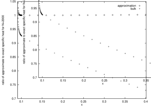
Figure 3:

Figure 4:

Figure 5:

Figure 6:

Figure 7:

Figure 8:

References

- [†] kirsten@tph100.physik.uni-leipzig.de.
- [‡] d.j.toms@newcastle.ac.uk.
- [1] S. N. Bose, Z. Phys. 26, 178 (1924).
- [2] A. Einstein, S. B. Preus. Akad. Wiss. 22, 261 (1924).
- [3] L. D. Landau and E. M. Lifshitz, Statistical Physics, Pergammon, London, 1969.
- [4] R. M. May, Phys. Rev. A 135, 1515 (1964).
- [5] F. London, Phys. Rev. 54, 947 (1938).
- [6] J. M. Blatt and K. W. Boer, Phys. Rev. 126, 1621 (1962).
- [7] S. A. Moskalenko, Sov. Phys. Solid State 4, 199 (1962).
- [8] L. L. Chase, N. Peyghambarian, G. Grynberg, and A. Mysyrowicz, Phys. Rev. Lett. 42, 1231 (1979); N. Peyghambarian, L. L. Chase, and A. Mysyrowicz, Phys. Rev. B 27, 2325 (1983); M. Hasuo et al., Phys. Rev. Lett. 70, 1303 (1993); J. Lin and J. P. Wolfe, ibid. 71, 1222 (1993).
- [9] M. H. Anderson, J. R. Ensher, M. R. Matthews, C. E. Wieman, and E. A. Cornell, Science 269, 198 (1995).
- [10] C. C. Bradley, C. A. Sackett, J. J. Tollett, and R. G. Hulet, Phys. Rev. Lett. 75, 1687 (1995).
- [11] K. B. Davis, M.-O. Mewes, M. R. Andrews, N. J. van Druten, D. S. Durfee, D. M. Kurn, and W. Ketterle, Phys. Rev. Lett. 75, 3969 (1995).
- [12] G. Baym and C. J. Pethick, Phys. Rev. Lett. 76, 6 (1996).
- [13] A. Fetter (unpublished).
- [14] F. Dalfovo and S. Stringari (unpublished).
- [15] S. R. de Groot, G. J. Hooyman, and C. A. ten Seldam, Proc. Roy. Soc. (London) A 203, 266 (1950).
- [16] V. Bagnato, D. E. Pritchard, and D. Kleppner, Phys. Rev. A 35, 4354 (1987).
- [17] S. Grossmann and M. Holthaus, Phys. Lett. A 208, 188 (1995).
- [18] S. Grossmann and M. Holthaus, Zeit. für Naturforschung 50 a, 921 (1995).
- [19] H. Haugerud and F. Ravndal, (unpublished), cond-mat/9509041.
- [20] See for example F. London, Superfluids II, (John Wiley, New York, 1954), K. Huang, Statistical Mechanics (John Wiley, New York, 1987) or R. K. Pathria, Statistical Mechanics (Pergammon, Oxford, 1972).
- [21] K. Kirsten and D. J. Toms, (unpublished), cond-mat/9604031.
- [22] M. R. Schafroth, Phys. Rev. 100, 463 (1955).
- [23] See R. K. Pathria, Can. J. Phys. 61, 228 (1983) for a review.
- [24] R. M. Ziff, G. E. Uhlenbeck and M. Kac, Phys. Rep. 32C, 169 (1977).
- [25] K. Kirsten and D. J. Toms, Phys. Lett. B 368, 119 (1996).
- [26] See H. R. Pajkowski and R. K. Pathria, J. Phys. A 10, 561 (1977), as well as Ref. [23] for a discussion of this subject.
- [27] K. Kirsten and D. J. Toms, Effective action approach to Bose-Einstein condensation of ideal gases, preprint, February 1996.
- [28] E. W. Barnes, Trans. Camb. Philos. Soc. 19, 426 (1903).
- [29] H. A. Weldon, Nucl. Phys. B 270, 79 (1986).
- [30] E. Elizalde and A. Romeo, Phys. Rev. D 40, 436 (1989).
- [31] L. Lewin, Dilogarithms and Associated Functions, (Mac Donald, London, 1958).
- [32] J. E. Robinson, Phys. Rev. 83, 678 (1951).
- [33] S. Grossmann and M. Holthaus, preprint, February 1996 (unpublished).
- [34] K. Kirsten and D. J. Toms, preprint, May 1996 (unpublished).
- [35] H. Haugerud, T. Haugset, and F. Ravndal, preprint, May 1996 (unpublished), cond-mat/9605100.
- [36] J. S. Dowker, J. Math. Phys. 35, 4989 (1994).
- [37] N. E. Nörlund, Acta Math. 43, 21 (1922).