[cond-mat/9607040] Training a perceptron by a bit sequence: Storage capacity

1 Introduction

Artificial neural networks are successful in predicting time series (Weigand et al 1993). Given a sequence of real numbers, a multilayer network is able to learn from $N$ consecutive numbers the following one. After learning a part of the sequence, the network is able to generalize: If $N$ consecutive numbers are taken from the part of the sequence which the network has not learned, the network can predict the following number to some extent.

Using methods and models of statistical mechanics, training from a set of examples and generalization of neural networks has been studied intensively (Hertz et al 1991, Kinzel et al 1991, Opper et al 1996). Most work has been concentrated on perceptrons and binary classification problems. A set of $N$ –dimensional input vectors is classified by a perceptron. A different perceptron is trained by this set of examples; after the training process the network is able to generalize: it has some overlap to the weights of the perceptron which has generated the examples. If the classification is not performed by a different perceptron but is assigned randomly, the network can still learn a certain amount of examples. The maximum number of examples, which can be classified by a perceptron, is related to the storage capacity of the corresponding attractor networks (Gardner 1988).

Only recently this approach has been extended to time series analysis (Eisenstein et al 1995) A perceptron was trained from a series of bits which was produced by a different perceptron. Hence also the generation of time series by a nerual network is interesting in this context, and recently an analytic solution of a stationary time series generated by a peceptron has been found (Kanter et al 1995).

It turns out that a perceptron can predict bit sequences very well, if those are taken from stationary time series produced by a different perceptron (Eisenstein et al 1995). Already a small training set leads to perfect prediction of the rest of the sequence, at least for $N\rightarrow\infty$ . However, the overlap between a learning and a generating network is very small.

In this paper we study the analogy of the storage capacity problem in the context of bit sequences: A set of $P$ consecutive bits, which are randomly chosen, is repeated periodically (or placed on a ring). A perceptron with $N<P$ is trained on this bit sequence, where the output bit is given by the bit which follows the $N$ input bits. Hence, the only difference to the examples used for the classification problem are correlations between the input and output: The output bit is contained in the input of $N$ examples.

In Section 2 we introduce the bit sequence, which we use for training a perceptron which is simulated in Section 3. Section 4 presents a signal to noise analysis of the Hebbian learning rule. A general Boolean function is considered in Section 5, and the last Section contains a summary and the conclusions.

2 Bit sequence

$P$ bits $S_{i}\in\{-1,1\};i=1,\dots,P$ are chosen randomly and independently. This sequence is repeated periodically from $i=-\infty$ to $i=\infty$ (or placed on a ring, equivalently). $N$ consecutive bits are used as an input to a perceptron with weights $w_{j}\in I\kern-4.2679pt{R};j=1,\dots,N$ (see Figure 1):

\sigma_{\nu}=\mathop{\rm sign}\nolimits\sum\limits^{N}_{j=1}\,w_{j}\,\xi^{\nu}_{j}\\ \mbox{with \,\,\,}\xi^{\nu}_{j}=S_{j-1+\nu}

(1)

The problem we are addressing here is the following: Can we find a weight vector $\underline{w}=(w_{1},\dots,w_{N})$ which reproduces the next bits in the sequence, i. e.

\sigma_{\nu}=S_{\nu+N}\mbox{\hskip 14.22636pt for all \hskip 14.22636pt}\nu\in I\kern-4.2679pt{N}\mskip 5.0mu plus 5.0mu.

(2)

In particular we are interested in the maximal number $P_{c}(N)$ of bits which can be reproduced correctly by a perceptron for $N\rightarrow\infty$ ; as usual we define

\alpha=P/N\mskip 5.0mu plus 5.0mu\mskip 5.0mu plus 5.0mu;\mskip 5.0mu plus 5.0mu\mskip 5.0mu plus 5.0mu\alpha_{c}=\lim_{N\rightarrow\infty}\mskip 5.0mu plus 5.0mu\mskip 5.0mu plus 5.0mu\frac{P_{c}(N)}{N}\mskip 5.0mu plus 5.0mu.

(3)

There exist mathematical theorems about the number configuration $\{\sigma_{\nu}\}$ which can be realized by Eq.(1), which are already more than 140 years old (Schläfli 1950, Cover 1965): If the $P$ input vectors $\underline{\xi^{\nu}}=(\xi^{\nu}_{1},\dots,\xi^{\nu}_{N})$ are in general position; i. e. if any subset of $N$ vectors is linearly independent, then the number $C(P,N)$ of possible configurations $\{\sigma_{\nu}\}\in\{+1,-1\}^{P}$ is given by

C(P,N)=2\sum\limits^{N-1}_{i=0}\,\,{P-1\choose i}\,.

(4)

In our case of the random bit sequence we expect the input vectors $\underline{\xi}^{\nu}$ to be in general position. For $P\leq N$ one obtains $C(P,N)=2^{P}$ ; hence, any bit sequence with $P\leq N$ can be perfectly predicted by a perceptron. For $P<2N$ there is still a large fraction of configurations which is given by Eq.(1); this fraction goes to one for $N\rightarrow\infty$ . This means that for random configurations $\{\sigma_{\nu}\}$ the probability to map them by a perceptron is one in the limit of $N\rightarrow\infty$ . For $P>2N$ this probability is zero. Hence, for a perceptron and random examples one finds $\alpha_{c}=2$ (Gardner 1988).

However, in our case the configurations $\{\sigma_{\nu}\}$ are not randomly chosen but taken from the input vectors. Each output bit $\sigma_{\nu}$ appears in $N$ input vectors $\underline{\xi}^{\nu+1},\dots,\underline{\xi}^{\nu+N}$ , too. There are correlations between the input vectors and the output bits. In addition, only the fraction of configuration $\sigma_{\nu}$ which cannot be reproduced by a perceptron goes to zero for $N\rightarrow\infty$ and $N<P<2N$ ; their number is still increasing exponentially with $N$ . For instance, for $N=100$ and $\alpha=1.8$ Eq.(4) gives about $10^{54}$ configurations which are not linearly separable, that is 6.7% of all of the possible $2^{180}$ ones. On the other side, for $P>2N$ the number of configurations which can be reproduced by a perceptron still increases exponentially with $N$ , although their fraction disappears. Hence, it is not obvious, whether the patterns given by a bit sequence belong to the first or second class, which means whether $\alpha_{c}<2$ or $\alpha_{c}>2$ .

In the uncorrelated case the storage capacity $\alpha_{c}$ has been calculated using the replica method (Gardner 1988). Correlations between the input vectors do not change the result $\alpha_{c}=2$ . Only if there is a bias for the output bits and for the input bits the storage capacity $\alpha_{c}$ increases with the bias. If the patterns are anticorrelated $\alpha_{c}$ can be lower than $\alpha_{c}=2$ , too (López et al 1995).

For our problem we have formulated the version space of weights in terms of replicas. One has to average over $P$ random bits, only, instead of $P\cdot N$ in the uncorrelated case. However, we did not succeed in getting rid of the correlations and could not solve the integral. Therefore, we have studied the bit sequence numerically.

3 Perceptron: Simulations

To calculate the storage capacity $\alpha_{c}$ of the perceptron being trained by a random bit sequence, we have used two methods:

(i)

We have used several routines which try to minimize the number of errors and indicate whether they did succeed or not. Hence, we obtained a fraction $f(\alpha,N)$ of patterns for which the routine could find a solution. The capacity $\alpha_{c}(N)$ is defined by $f(\alpha_{c},N)=1/2$ . Obviously, we obtain a lower bound for the true $\alpha_{c}$ , only. The results did not dependent on the actual algorithm within the expected error bounds.

We have used a routine that minimizes the “linear cost-function” $E=\sum_{\nu=0}^{P}\mathop{\theta}\nolimits(1-E^{\nu})(1-E^{\nu})$ with $E^{\nu}={1\over N}\sum_{j=1}^{N}w_{j}\xi_{j}^{\nu}\sigma^{\nu}$ (without constraining the vector $\underline{w}$ ).
(ii)

The other estimate uses the median learning time (Priel et al 1994). For random patterns the average learning time $\tau_{a}$ of the perceptron algorithm diverges as $\tau_{a}^{-1/2}\sim(\alpha_{c}-\alpha)$ for $\alpha\rightarrow\alpha_{c}$ (Opper 1988). We use this power law in our case, too. The median $\tau_{m}$ of the distribution of learning times is calculated for $\alpha<\alpha_{c}$ and $\alpha_{c}$ is obtained from a fit to the power law divergence. This method has the advantage that one does not have to determine whether a pattern cannot be learned at all. If the number of learning steps is larger than the median the algorithm can stop; this saves a large amount of computer time.

Figure 2 and Table 1 show the results of the simulations ²²2Preliminary results have been reported 1994 by Bork. In the uncorrelated case both of the methods give the exact result $\alpha_{c}=2$ within the statistical error and for $N=100$ , already. If we use the input from the bit sequence but random output bits the results agree with $\alpha_{c}=2$ , too. However, if in addition we use the output bits from the bit sequence we obtain $\alpha_{c}=1.70\pm 0.02$ . Hence, the correlations between output bits and input vectors decrease the storage capacity. For the perceptron it is harder to learn a random bit sequence than a random classification problem. This is due to the correlations between input and output but not due to the correlations between the input vectors.

If a perceptron which has learned a bit sequence perfectly is used as a bit generator, then any initial state of $N$ bits taken from the sequence reproduces the complete sequence. Hence the sequence is an attractor of the bit generator. However we found, that the basin of attraction is very small. If only one bit is flipped in the initial state then there is a high probability that the generator runs into a different sequence.

We have also studied two additional problems:

(i)

The $P$ random bits are not repeated periodically but the perceptron is trained with a string of $N+P$ random bits. Hence, there are still $P$ patterns but an output bit belongs only to part of the other input patterns. On average the correlations are weaker. Indeed, we find that the storage capacity $\alpha_{c}=1.82\pm 0.02$ is larger than the one for the periodic sequence.
(ii)

With a bias $m=\frac{1}{p}\,\sum\limits^{P}_{i=1}\,S_{i}$ in the bit sequence, the storage capacity increases. This is similar to the random classification problem (Gardner 1988).

4 Perceptron: Hebbian learning rule

In order to get some insight from analytic calculations we now consider the Hebbian learning rule

\underline{w}=\frac{1}{N}\,\sum\limits^{P}_{\nu=1}\,\sigma_{\nu}\underline{\xi}^{\nu}\,.

(5)

Output bits $\sigma_{\nu}$ and input vectors $\underline{\xi}^{\nu}$ are taken from a bit sequence $\{S_{i}\}$ , Eqs.(1) and (2). It is known that the Hebbian weights cannot map the examples perfectly. However, the training error can be calculated from a signal to noise analysis (see for instance Hertz et al 1991). The sign of the following stability $E^{\nu}$ shows whether an example is classified correctly.

E^{\nu}=\sigma^{\nu}\underline{w}\underline{\xi}^{\nu}=\frac{1}{N}\,\sum\limits^{N}_{i=1}\,\sum\limits^{P}_{\mu=1}\,\sigma^{\nu}\,\sigma^{\mu}\xi^{\nu}_{i}\xi^{\mu}_{i}\,.

(6)

The fraction of negative values of $E^{\nu}$ defines the training error.

We calculated the first two moments $\langle E\rangle$ and $\langle E^{2}\rangle$ of $E^{\nu}$ , where $\langle\dots\rangle$ means an average over the distribution of the examples, i.e. over all realizations of the bit sequence. If all bits $\sigma_{\nu}$ and $\xi^{\nu}_{i}$ are random one has

\langle\sigma^{\nu}\sigma^{\mu}\rangle=\delta_{\nu\mu}\mskip 5.0mu plus 5.0mu\mskip 5.0mu plus 5.0mu;\mskip 5.0mu plus 5.0mu\mskip 5.0mu plus 5.0mu\langle\xi^{\nu}_{i}\xi^{\mu}_{j}\rangle=\delta_{\nu\mu}\delta_{i\,j}\,.

(7)

This gives

$\displaystyle\hskip 72.0pt{\langle E\rangle=1\mskip 5.0mu plus 5.0mu\mskip 5.0mu plus 5.0mu;\mskip 5.0mu plus 5.0mu\mskip 5.0mu plus 5.0mu\langle E^{2}\rangle=1+\alpha\,.}$

In the limit $N\rightarrow\infty$ the values of $E^{\nu}$ are Gaussian distributed with mean $1$ and standard deviation $\sqrt{\alpha}$ . However, for the periodic bit sequence, Eqs. (1) and (2), the values of $\sigma^{\nu}$ and $\xi^{\nu}_{j}$ are taken from the random bits $S_{i}$ . For instance $\sigma^{\nu}$ is identical with $\xi^{\mu}_{j}$ for $j=1,..,N$ and $\mu=\nu+N+1-j$ . Taking this into account we find for $1<\alpha<2$ :

\begin{array}[]{ccl}\langle E\rangle&=&\left\{\,\vbox{\openup 3.0pt\halign{\strut$\displaystyle{#}\hfil$&\tqs\rm#\hfil\cr 1+\frac{1}{N}&\hskip 25.0pt\rm for $P$ even\cr 1&\hskip 25.0pt\rm for $P$ odd\cr}}\right.\\[14.22636pt] \langle E^{2}\rangle&=&\left\{\,\vbox{\openup 3.0pt\halign{\strut$\displaystyle{#}\hfil$&\tqs\rm#\hfil\cr 2+\alpha+\frac{6-\alpha}{N}-\frac{4}{N^{2}}&\hskip 25.0pt\rm for $P$ even\cr 2+\alpha-\frac{2}{N}&\hskip 25.0pt\rm for $P$ odd\cr}}\right.\end{array}

(8)

For $\alpha>2$ the results above for odd $P$ hold for even ones, too. Hence for $N\rightarrow\infty$ the standard derivation of the $E^{\nu}$ values is $\sqrt{1+\alpha}$ instead of $\sqrt{\alpha}$ of the uncorrelated case. The correlations increase the noise relatively to the signal. Assuming a Gaussian distribution of the $E^{\nu}$ values in the limit $N\rightarrow\infty$ , which is supported by our numerical simulation, we obtain the training error $\varepsilon_{t}$ as

\varepsilon_{t}=\phi\left(-\frac{1}{\sqrt{1+\alpha}}\right)

(9)

with the error function

\phi(x)=\int\limits^{x}_{-\infty}\,\frac{1}{\sqrt{2\pi}}\,e^{-\frac{y^{2}}{2}}dy\,.

(10)

If the random bits are not repeated periodically, but arranged linearly as discussed above, the moments depend on the number $\nu$ of the pattern. If $\nu=1$ is the first and $\nu=P$ is the last pattern, we define

\gamma=\left\{\begin{array}[]{ccc}\nu/N&\mbox{ for }&\nu\leq N\\ 1&\mbox{ for }&\nu>N\end{array}\right.

(11)

In this case the training error depends on $\gamma$ and we find

\varepsilon_{t}=\phi\left(-\frac{1}{\sqrt{\alpha+\gamma^{2}}}\right)\,.

(12)

Figure 3 shows the training error $\varepsilon_{t}(\alpha)$ for the uncorrelated bits and the periodic bit sequence. In the latter case $\varepsilon_{t}$ is averaged over the patterns. The correlations of the bit sequence increase the training error, in agreement with the decrease of the storage capacity shown in the previous section.

5 General Boolean function

Up to now we have restricted our map to a perceptron. We expect that multilayer networks can reproduce a larger bit sequence, in accordance to the higher storage capacity of the committee machine (Priel et al 1994). In this section we study the storage capacity of a general Boolean function $b:\{+1,-1\}^{N}\rightarrow\{+1,-1\}$ , which is the size of the random bit sequence with period $P$ which can be reproduced by any Boolean function $b$ , i.e.

b(S_{\nu},\dots,S_{\nu+N-1})=S_{\nu+N}\,;\,\nu=1,\dots,P\,.

(13)

Since we have the freedom to choose for any input configuration $(S_{\nu},\dots,S_{\nu+N-1})$ an arbitrary output bit $S_{\nu+N}$ , our problem reduces to the question if all of the input configurations are different from each other. If all $(S_{\nu},\dots,S_{\nu+N-1})$ are different then we can define a Boolean function which maps each of those states to the corresponding bit $S_{\nu+N}$ . For the rest of the $2^{N}-P$ input states we have the freedom to choose an arbitrary output bit; hence in this case, there are $2^{(2^{N}-P)}$ many Boolean functions which map the bit sequence correctly.

If two of the input configurations $(S_{\nu},\dots,S_{\nu+N-1})$ are identical there is still a probability of $1/2$ that the two output bits are different, too. To get an analytic estimate for the size of a random bit sequence which can be reproduced by a Boolean function we neglect correlations between the input configurations. That means we consider $P$ configurations $(S_{1}^{\nu},\dots,S_{N}^{\nu})\,;\,\nu=1,\dots,P$ where all of the bits $S^{\nu}_{i}$ are chosen randomly and independently. We want to calculate the probability $f$ that all of the $P$ states are pairwisely different. There are $2^{N}$ many possible states. The first configuration $\nu=1$ can be any of those states. The second one can take any of the $2^{N}-1$ remaining states, etc. Hence, the number $C$ of allowed configurations is

C=2^{N}(2^{N}-1)(2^{N}-2)\cdots(2^{N}-P+1)

(14)

which gives

	$\displaystyle\ln C$	$\displaystyle=\sum\limits^{P}_{\nu=1}\,\ln(2^{N}-\nu+1)=\sum\limits^{P}_{\nu=1}\left[N\ln 2+\ln\left(1-\frac{\nu-1}{2^{N}}\right)\right]$			(15)
		$\displaystyle=PN\ln 2+\sum\limits^{P}_{\nu=1}\,\ln\left(1-\frac{\nu-1}{2^{N}}\right)\,.$			(16)

If $P\ll 2^{N}$ we can expand $\ln$ and obtain

\ln C\simeq PN\ln 2-\frac{1}{2^{N}}\,\frac{P(P-1)}{2}\,.

(17)

Since the total number of all possible configurations is $2^{PN}$ , the function of the allowed ones is

f\simeq\exp\left[-\frac{P(P-1)}{2^{N+1}}\right].

(18)

We define the average period $P_{c}$ by $f(P_{c})=1/2$ and obtain for large $N$

P_{c}=\sqrt{2\ln 2}\,\,\,2^{\frac{N}{2}}\,.

(19)

Hence we expect that the average length of the bit sequence which can be reproduced by a Boolean function scales as the square root of $2^{N}$ . In fact our problem is similar to the random map, where the average cycle length has the same scaling property (Harris 1960, Derrida et al 1987).

The configurations taken from a random bit sequence are correlated, since consecutive configurations are obtained by shifting a window of $N$ bits over the sequence. However, our numerical simulations show that these correlations do not change the scaling law Eq.(19). For a given sequence with $P$ bits the size $N$ of the window is increased until this sequence can be reproduced by a Boolean function. $N_{c}$ is defined as the window size $N$ where 50% of the sequences are reproduced. In Figure 4, $P$ is shown as a function of $N_{c}$ . For $P\leq 17$ , $N_{c}$ is determined by exhaustive enumeration. For larger $P$ values $N_{c}$ is estimated from up to $10^{5}$ random samples. The log-linear plot shows that the data are consistent with

P=1.6\times\sqrt{2}^{N_{c}}\,.

(20)

The comparison with Eq.(19) shows that the correlations seem to change the prefactor from $1.17$ to $1.6$ , but the number still increases with the square root of $2^{N}$ , the size of the input space.

6 Summary

A perceptron of $N$ input bits has been trained by a random bit sequence with a period $P$ . Each output bit is contained in $N$ input vectors. These correlations decrease the storage capacity to $\alpha_{c}=1.7\pm 0.02$ compared to $\alpha_{c}=2$ for uncorrelated output bits. For the corresponding bit generator the bit sequence has a tiny basin of attraction.

An analysis of Hebbian weights shows that a bit sequence gives a larger noise to signal ratio than a random classification problem. This result is in agreement with the lower storage capacity.

If a general Boolean function is trained by the random bit sequence, the maximal period $P$ scales as the square root of $2^{N}$ , the size of the input space.

Acknowledgements

This work has been supported by the Deutsche Forschungsgemeinschaft and the MINERVA center of physics of the Bar-Ilan University. We thank Georg Reents for valuable discussions.

References

Bork A 1994 Zeitreihenanalyse Diploma thesis (Würzburg: Institut für Theoretische Physik der Universität Würzburg)
Cover T M 1995 IEEE Trans. Electron. Comput. EC-14 326
Derrida B and Flyvbjerg 1987 J. Physique 48 971
Eisenstein E, Kanter I, Kessler D A and Kinzel W 1995 Phys. Rev. Lett. 74 6
Fontanari JF and Meir R 1989 J. Phys. A: Math. Gen. 22 L803
Gardner E 1988 J. Phys. A: Math. Gen. 21 257
Harris B 1960 Ann. Math. Stat. 31 1045
Hertz J, Krogh A and Palmer R G 1991 Introduction to the theory of neural computation (Redwood City, CA: Addison Wesley)
Kanter I, Kessler D A, Priel A and Eisenstein E 1995 Phys. Rev. Lett. 75 2614
Kinzel W and Opper M 1991 in Models of Neural Networks eds. Domany E, van Hemmen J L and Schulten K (Berlin: Springer) p 149
López B, Schröder M and Opper M 1995 J. Phys. A: Math. Gen. 28 L447
Monasson R 1992 J. Phys. A: Math. Gen. 25 3701
Opper M 1988 Phys. Rev. A 38 3824
Opper M and Kinzel W 1996 in Models of Neural Networks III eds. Domany E, van Hemmen J L and Schulten K (New York: Springer) p 151
Priel A, Blatt M, Grossmann T and Domany E 1994 Phys. Rev. E 50 577
Schläfli L 1950 in Ludwig Schläfli 1814–1895: Gesammelte Mathematische Abhandlungen ed. Steiner-Schläfli-Komitee (Basel: Birkhäuser) 171
Tarkowski W and Lewenstein M 1993 J. Phys. A: Math. Gen. 26 2453
Weigand A S and Gershenfeld N A (eds) 1993 Time Series Prediction, Forecasting the Future and Understanding the Past (Santa Fe: Santa Fe Institute)

Figure 1

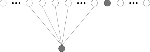
Refer to caption — Figure 1: A perceptron learning a periodic time series. The desired output of the perceptron (marked) is the next bit of the series and therefore part of other input patterns as well.

Figure 2

Figure 3

Figure 4

$\log P$ $N_{c}$

Table 1: The storage capacity of a perceptron learning different tasks. Measured with (1) half-error and (2) median learning-time method

	method 1	method 2
random $N=100$	$1.99\pm 0.01$	$1.995\pm 0.01$
time series $N=100$	$1.85\pm 0.025$	$1.82\pm 0.02$
time series $N=400$		$1.82\pm 0.02$
ring $N=100$	$1.7\pm 0.025$	$1.69\pm 0.01$
ring $N=400$		$1.7\pm 0.02$
ring (rnd out) $N=100$	$1.98\pm 0.05$	$1.99\pm 0.01$
ring (rnd out) $N=400$		$1.98\pm 0.02$
magnetization $m=0.4$	$N=100$
ring	$1.95\pm 0.05$	$1.95\pm 0.03$
random	$2.25\pm 0.05$

Training a perceptron by a bit sequence: Storage capacity

Abstract

pacs: