[

Traveling-Wave Chemotaxis

Abstract

A simple model is studied for the chemotactic movement of biological cells in the presence of a periodic chemical wave. It incorporates the feature of adaptation that may play an important role in allowing for “rectified” chemotaxis: motion opposite the direction of wave propagation. The conditions under which such rectification occurs are elucidated in terms of the form and speed of the chemical wave, the velocity of chemotaxis, and the time scale for adaptation. An experimental test of the adaptation dynamics is proposed.

]

Many biological processes involve chemotaxis, cellular motion in response to a chemical stimulus. Often, the chemo-attractant propagates through a set of cells as traveling waves [2, 3], as in a case of longstanding interest: the emergence of a multicellular structure from colonies of the eukaryotic microorganism Dictyostelium discoideum (Dd)[4]. In controlled experiments, a monolayer with $10^{5}-10^{6}$ cells/cm² on the surface of agar begins within several hours after nutrient deprivation to support waves of cyclic adenosine monophosphate (cAMP) triggered by spontaneous release of cAMP from a small subpopulation of cells. These target or rotating spiral waves (Fig. 1), whose fronts appear as bands under dark-field visualization through their effects on cell shape [5], induce chemotaxis toward their centers, followed by complex multicellular morphogenesis.

Chemical waves in excitable media such as Dd are quite thoroughly explored [6, 7], but their coupling to cell density through chemotaxis is far less well-understood, although of longstanding interest [8, 9, 10]. As emphasized recently [11], and illustrated in Fig. 1a [12], chemotaxis driven by traveling waves is quite intriguing. A cell in the position indicated by the arrow experiences a progression of leftward-moving wavefronts as the nearby spiral rotates outward. In seeking higher levels of cAMP, the cell would move first rightward into each advancing wave, then leftward after the peak has passed (Fig. 1b). In the simplest model of chemotaxis, the cell velocity is proportional to the local chemical gradient, and it has been argued [11] (but not proven theoretically) that the net cellular motion would be in the same direction as the wave: i.e. “advection” away from the center, rather than the observed motion towards the spiral core. Tracking studies of cells [11] suggest a resolution to this by noting that as the cells experience the rising cAMP level of the approaching wave, their chemotactic response diminishes, leaving them less responsive to the trailing edge, but their response recovers in time for the next front. They thus rectify the traveling waves, with net motion opposite that of the wave.

In an effort to understand the underlying mechanism of this process, we study here a very simple model for “adaptive” traveling-wave chemotaxis and suggest experiments to test its predictions for the conditions under which rectification occurs. This model is closely related to, but considerably simpler than one introduced recently in important work by Höfer, et al. [13], who demonstrated by numerical computations that a process of adaptation could lead to rectified motion. A number of important aspects of this problem become clear with these simplifications, particularly in the experimentally relevant limit of chemotactic velocities small compared to the wave speed. First, in this limit an elementary proof is given of the heuristic argument [11] that nonadaptive chemotaxis will not produce rectified motion. Second, it is shown that rectified motion requires only two main

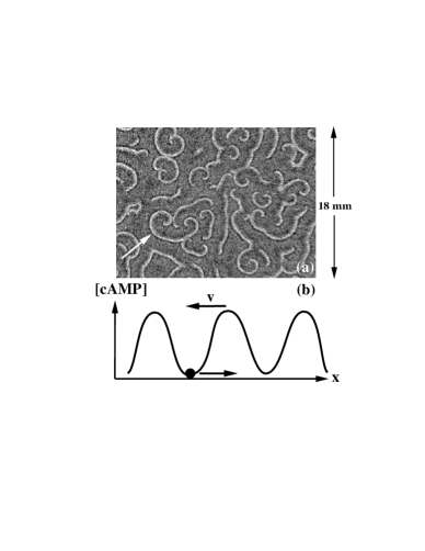
FIG. 1.: (a) Dark-field image of spiral waves in Dictyostelium discoideum [12]. Wavefronts of cAMP appear as dark bands. A cell in the position indicated experiences a periodic train of cAMP waves, shown schematically in (b). Net chemotactic motion occurs toward the spiral core, opposite the direction of wave propagation.

ingredients: (i) a single characteristic time for adaptation, and (ii) a response function that decreases with concentration.

Third, the net chemotactic flux is shown to have a thermodynamic analogy in being proportional to the area enclosed by certain limit cycles exhibited in the response-concentration plane. Fourth, an analytical calculation confirms the intuitive notion that rectification is greatest when the adaptation time is comparable to the wave period (as seen in experiment [11]), although there can be a delicate interplay between the competing processes of rectification and advection. Finally, an experimental test of these results is suggested.

Consider a one-dimensional set of noninteracting cells at density $\rho$ responding to a periodic chemical concentration wave $c(x,t)\equiv c(x+vt)$ with wavelength $\lambda$ and velocity $v$. Typically, $\lambda\sim 0.1-0.5$ cm (Fig. 1), and $v\sim 10^{2}-10^{3}$ $\mu$m/min. We leave aside the complex dynamics of wave production and its connection to the cell density [14, 15, 16]. The model is formulated at the level of the coordinate $x(t)$ of a cell, and for the present purposes is deterministic, as the random motions of the cells during one wave period are small on the scale of the wavelength $\lambda$. Deterministic chemotaxis arising from chemical gradients is described by the overdamped dynamics

$${dx\over dt}=r{d\over dx}c(x+vt)~{}.$$ (1)

The chemotactic response coefficient $r$ measures the strength of chemotaxis, with cells migrating to high values of $c$ when $r>0$. When $r$ responds to $c$ we have “adaptive chemotaxis”; otherwise the motion is nonadaptive. The flux of cells $\langle J\rangle$ ($=(1/\lambda)\int_{0}^{\lambda}dzJ$) averaged over one wave period is found by solving (1) in the moving frame $z=x+vt$, with $dz/[r(dc/dz)+v]=dt$, and transforming back (see also [17]),

$${\cal J}\equiv\langle J\rangle/\rho v=\left<\left[1+r\left(dc/dz\right)/v\right]^{-1}\right>^{-1}-1~{}.$$ (2)

It is known from experiment that the typical chemotactic velocity $rdc/dz$ in Dd is at least an order of magnitude lower than the wave speed $v$ [2, 13], so we expand ${\cal J}$ in powers of $v^{-1}$,

$${\cal J}\simeq{1\over v}\left<r{dc\over dz}\right>-{1\over v^{2}}\left[\left<\left(r{dc\over dz}\right)^{2}\right>-\left<r{dc\over dz}\right>^{2}\right]~{}.$$ (3)

In nonadaptive chemotaxis, $r$ is constant, so the first term vanishes by the periodicity of $c(z)$. The first nonvanishing contribution to ${\cal J}$ is in the direction of the wave propagation, independent of the form of $c(z)$ since the variance of $rdc/dz$ is manifestly positive. This confirms the heuristic argument of Wessels, et al. [11]. The physical basis for this was emphasized in the context of Brownian particles forced by moving optical traps [17]: Particles migrating into the advancing wave experience the leading edge (and hence chemotax) for a shorter time than they do the trailing edge, since their velocity relative to the wave is greater in the former case than in the latter. One step forward, two steps back, so to speak.

A very simple adaptive chemotaxis model has two ingredients: (i) an equilibrium “adaptation function” $f(c)$ that is a decreasing function of $c$, and (ii) a single time constant $\tau$ for the relaxation of $r$ toward $f$ [18],

$$\tau{dr\over dt}=f(c)-r~{}.$$ (4)

A cell having experienced a concentration $c$ for times much longer than $\tau$ will have a response coefficient $r=f(c)$ when next presented with a gradient: low when $c$ is high, and vice versa. As $c$ changes with time the response will attempt to equilibrate to $f(c)$, but will lag behind when $c$ changes on time scales shorter than $\tau$. One can think of this lag as a memory or inertial effect, and it provides a means of rectification. We expect the adaptation time to be comparable to the refractory period of cAMP signaling. Eq. 4 is one member of a FitzHugh-Nagumo model that has been studied in related work on chemotaxis [10].

Let us introduce the dimensionless coordinate $Z=kz$, time $T=\omega t$, concentration $C=c/c_{0}$, response coefficient $R=r/f_{0}$, and adaptation function $F=f/f_{0}$, where $k=2\pi/\lambda$, $\omega=kv$, $c_{0}$ is the peak wave concentration, and $f_{0}\equiv f(c=0)$. The rescaled dynamics are

$${dZ\over dT} = SR{dC\over dZ}+1$$ (6)

$$\Omega{dR\over dT} = F(C)-R~{},$$ (7)

with two dimensionless parameters,

$$\Omega=\omega\tau~{},\ \ S=f_{0}c_{0}k/v~{}.$$ (8)

The quantity $\Omega$ measures the relaxation time in units of the wave period, while $S$ is the ratio of a characteristic chemotactic speed to the wave speed.

The expansion of the average flux in Eq. (3) now appears as an expansion in $S$, with the ${\cal O}(S)$ term possibly rectifying, and those of order $S^{2}$ always advective. For a given value of $S$, we expect three regimes of $\Omega$: (i) $\Omega\gg 1$, the nonadaptive case already discussed, (ii) $\Omega\simeq 1$, where rectification may occur, and (iii) $\Omega\ll 1$, with instantaneous adaptation. In region (iii), the response tracks the concentration precisely, and the leading and trailing sides of the wave are not distinguished, so the flux is positive and given analytically by Eq. (2) with $r$ replaced by $f(c)$. It is smaller than in (i) since $f(c)$ is smaller for high $c$. Rectification may occur in region (ii), where the down-regulation of the response triggered by the advancing wave has not fully recovered by the time the trailing edge is encountered.

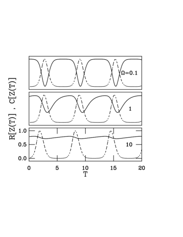
FIG. 2.: Relation between morphogen concentration and chemotactic response. Panels show the imposed chemical wave $C(Z(T))$ (dashed) and the response coefficient $R(Z(T))$ (solid) for $S=0.2$ and various scaled frequencies $\Omega$.

Figure 2 shows for different values of $\Omega$ the concentration $C$ and response coefficient $R$ as functions of time along the trajectory of a moving cell obtained by numerical integration of (1). An arbitrary initial condition decays in a time of order $\Omega$ into the steady patterns shown. To simulate the sharply-peaked traveling waves seen in experiment, we chose $C(Z)=\exp\left[\beta\left(\sin(Z)-1.0\right)\right]$, with $\beta=3.0$. The response function is the simplest: a linearly decreasing function of $C$: $F(C)=1-C$. For $\Omega=0.1$ (close to instantaneous adaptation) we see $R$ almost precisely anticorrelated with $C$, whereas for $\Omega\simeq 1$ the asymmetric response between leading and trailing edges is quite apparent. For $\Omega=10$ the response settles to a nearly constant value determined by the mean value of the concentration over one wave period.

The extent to which the response is “out of equilibrium” is seen with limit cycles in the $R-C$ phase plane shown in Fig. 3, with position $Z$ as a parameter. For small $\Omega$ the cycle hugs the equilibrium curve $F(C)$, while when $\Omega\gg 1$ it is a narrow loop encircling a horizontal line of constant $R$. In the rectifying regime ($\Omega=1$) the cycle lies very far from equilibrium, forming a large closed loop. Using the high-velocity result in Eq. (3), we may express the chemotactic flux directly in terms of the area enclosed by this loop ${\cal C}$,

$${\cal J}\simeq{S\over 2\pi}\int_{0}^{2\pi}\!dZR{dC\over dZ}={S\over 2\pi}\oint_{{\cal C}}RdC~{},$$ (9)

in much the same way as we associate mechanical work with loops in the pressure-volume plane. With the sense of traversal of the loops shown in Fig. 3 this area is positive, and hence rectifying. With these results, we obtain the chemotactic flux shown in Fig. 4, highlighting the window around $\Omega=1$ within which rectification occurs. For $S$ small rectification occurs over almost the entire range of $\Omega$, since advection is negligible. But for larger

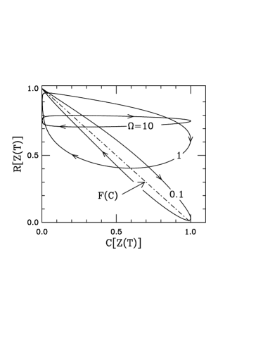
FIG. 3.: Phase portrait of traveling-wave chemotaxis. Data in Fig. 2 are replotted in the $R-C$ plane. The equilibrium function $F(C)$ is shown dashed. Arrows indicate sense of traversal with increasing time.

$S$ advection dominates at the extremes of $\Omega$, and rectification occurs in a very narrow window near $\Omega=1$. The qualitative behavior seen in Figs. 2-4 is unchanged by the inclusion of more complicated nonlinear adaptation functions more faithful to the biochemistry of receptor binding [13].

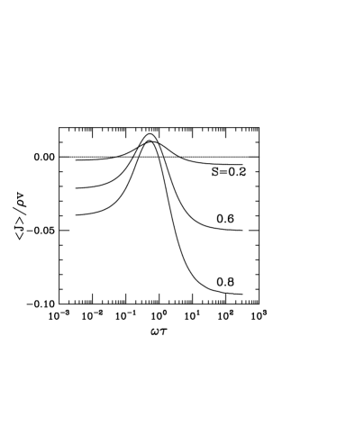
FIG. 4.: Flux as a function of relaxation time and chemotactic velocity. At low $S$, rectification occurs over a broad range of $\Omega$, while at higher $S$ advection is dominant except over a narrow range of $\Omega\simeq 1$.

Insight into the quantitative behavior of the model may be obtained by an analytic calculation in the limit of large wave speeds (small $S$) [13]. We assume an expansion of the position $Z$ and response coefficient $R$ in powers of $S$: $Z(T)=Z^{(0)}(T)+SZ^{(1)}(T)+\cdots$ and $R(T)=R^{(0)}(T)+SR^{(1)}(T)+\cdots$. At order $S^{0}$ in this moving coordinate system we obtain $dZ^{(0)}/dT=1$, so $Z^{(0)}(T)=T$. At order $S$ we obtain the equation of motion of a particle due to a time-dependent force

$${dZ^{(1)}\over dT}=R^{(0)}(T){dC(T)\over dT}~{},$$ (11)

$$R^{(0)}(T)={1\over\Omega}\int^{T}\!dT^{\prime}{\rm e}^{-(T-T^{\prime})/\Omega}F(C(T^{\prime}))~{}.$$ (12)

We continue with the simple model $F(C)=1-C$. If $C(Z)$ has the Fourier expansion $C(Z)=\bar{C}+\sum_{n=1}^{\infty}\left[\alpha_{n}\exp(inZ)+c.c.\right]$, then after the transients the modes of $R$ are shifted in phase from the wave,

$$R^{(0)}(T)=1-\bar{C}-\sum_{n=1}^{\infty}{\alpha_{n}{\rm e}^{i(nT-\theta_{n})}+c.c.\over\sqrt{1+(n\Omega)^{2}}}~{}.$$ (13)

The phase shifts $\theta_{n}$ satisfy $\tan\theta_{n}=n\Omega$, and thus are nearly zero for instantaneous adaptation and tend to $\pi/2$ as $\Omega\to\infty$, more rapidly with increasing mode number $n$. To compute the flux in this small-$S$ limit, we find the mean value of $R^{(0)}(T)dC/dZ$ over one period,

$${\cal J}\sim{S\over 2\pi}\sum_{n=1}^{\infty}n\sin(2\theta_{n})\left|\alpha_{n}\right|^{2}~{},$$ (14)

where $\sin(2\theta_{n})=2n\Omega/(1+(n\Omega)^{2})$. The generic behavior of this sum is seen from its first term, which vanishes as $\Omega\to 0$ and $\Omega\to\infty$, and peaks at $\Omega=1$ to give maximum forward flux. When the wave has dominant spectral weight in a higher mode $n$, the peak in flux will occur for $\Omega\sim 1/n$, as in Fig. 4. Once we go beyond the limit of vanishing $S$, the negative contributions to the flux (3) compete with the rectifying part to produce the resonance-like behavior seen in Fig. 4.

We see that rectified chemotactic motion requires only two simple ingredients: a single time scale for adaptation, and an adaptation function that decreases with concentration. Adaptive phenomena are found in many biological systems besides D. discoideum, including those of bacterial chemotaxis [19]. While this problem may appear similar to ones of directional transport studied recently in the context of electrophoresis [20], there is a fundamental distinction; the rectified motion arises here through processes internal to the particles, not through stochasticity. Indeed, the random motions of cells are expected to decrease the efficiency of rectification. Finally, these results suggest experiments to probe the competition between advective and adaptive chemotaxis (Fig. 4) with artificially-produced chemical waves of controllable shape and velocity [21], complementary to recent experiments with fixed gradients [22] and time-varying uniform concentrations [11]. Observation of the predicted advection with a wave whose frequency is either very small or very large compared to the natural signalling frequency would provide important evidence that adaptation associated with an internal time scale is the operative mechanism in rectified chemotaxis.

I am indebted to J.T. Bonner, E.C. Cox, K.J. Lee, R.H. Austin, and P. Nelson for many discussions, to P. Holmes, and C.H. Wiggins for suggestions, and to A. Goriely for pointing out the work of Hofer, et al.. This work was supported by NSF PFF grant DMR 93-50227, and the A.P. Sloan Foundation.

REFERENCES

- [1] Electronic mail: gold@davinci.princeton.edu
- [2] Biology of the Chemotactic Response, Ed. by J.M. Lackie and P.C. Wilkinson (Cambridge University Press, New York, 1981).
- [3] See e.g. Oscillations and Morphogenesis, Ed. by L. Rensing (Marcel Dekker, New York, 1993); Cell-to-Cell Signalling: From Experiments to Theoretical Models, Ed. by A. Goldbeter (Academic Press, New York, 1989).
- [4] J.T. Bonner, The Cellular Slime Molds, 2nd ed. (Princeton University Press, Princeton, NJ 1967).
- [5] cAMP waves are directly visualizable by fluorographic means; K.J. Tomchik and P.N. Devreotes, Science 212, 443 (1981).
- [6] For a review, see E. Meron, Phys. Rep. 218, 1 (1992).
- [7] J.J. Tyson and J.D. Murray, Development 106, 421 (1989).
- [8] E.F. Keller and L.A. Segel, J. Theor. Biol. 30, 225, 235 (1971); M.H. Cohen and R. Robertson, ibid. 31, 119 (1971).
- [9] H. Levine and W. Reynolds, Phys. Rev. Lett. 66, 2400 (1991).
- [10] B.N. Vasiev, P. Hogeweg, and A.V. Panfilov, Phys. Rev. Lett. 73, 3173 (1994).
- [11] D. Wessels, J. Murray, and D.R. Soll, Cell Motility and the Cytoskeleton 23, 145 (1992). See also B.J. Varnum-Finney, E. Voss, and D.R. Soll, ibid. 8, 18 (1987); B. Varnum-Finney, N.A. Schroeder, and D.R. Soll, ibid. 9, 9 (1988).
- [12] K.J. Lee, E.C. Cox, and R.E. Goldstein, Phys. Rev. Lett. 76, 1174 (1996).
- [13] T. Höfer, P.K. Maini, J.A. Sherratt, M.A.J. Chaplain, P. Chauvet, D. Metevier, P.C. Montes, and J.D. Murray, Appl. Math. Lett. 7, 1 (1994).
- [14] M.H. Cohen and A. Robertson, J. Theor. Biol. 31, 101 (1971)
- [15] J.L. Martiel and A. Goldbeter, Biophys. J. 52, 807 (1987).
- [16] P.B. Monk and H.G. Othmer, Phil. Trans. R. Soc. London B 323, 185 (1989).
- [17] L.P. Faucheux, G. Stolovitzky, and A. Libchaber, Phys. Rev. E. 51, 5239 (1995).
- [18] Ref. [10] describes a more complicated model of chemotactic response with thresholds, while Ref. [13] incorporates concentration-dependent rate constants and highly nonlinear concentration-response relations.
- [19] J.A. Shapiro, BioEssays 17, 597 (1995).
- [20] J. Rousselet, L. Salome, A. Ajdari, and J. Prost, Nature (London) 370, 447 (1994).
- [21] R.H. Austin, private communication (1995).
- [22] P.R. Fisher, R. Merkl, and G. Gerisch, J. Cell Biology 108, 973 (1989).