Monte Carlo simulation of a two-dimensional continuum Coulomb gas

Abstract

We study the classical two-dimensional Coulomb gas model for thermal vortex fluctuations in thin superconducting/superfluid films by Monte Carlo simulation of a grand canonical vortex ensemble defined on a continuum. The Kosterlitz-Thouless transition is well understood at low vortex density, but at high vortex density the nature of the phase diagram and of the vortex phase transition is less clear. From our Monte Carlo data we construct phase diagrams for the 2D Coulomb gas without any restrictions on the vortex density. For negative vortex chemical potential (positive vortex core energy) we always find a Kosterlitz-Thouless transition. Only if the Coulomb interaction is supplemented with a short-distance repulsion, a first order transition line is found, above some positive value of the vortex chemical potential.

I Introduction

Physical systems, which are effectively two dimensional and whose important thermal excitations are vortices, can undergo a Kosterlitz-Thouless (KT) transition [1]. A prototype model for such systems is the two-dimensional Coulomb gas (2D CG), and it is well known to have two distinct phases. In the low temperature phase vortices are present only in tightly bound vortex-antivortex pairs (vortex insulator). In the high temperature phase, above the KT transition temperature, free vortices are present (vortex metal). Examples of such physical systems are: thin-film superconductors, two-dimensional superfluids, Josephson-junction arrays, two-dimensional melting, and double layer quantum Hall systems, etc [2, 3, 4]. The KT transition has been studied theoretically in detail, but few rigorous results are established and some important uncertainties remain. Notably, how good are the renormalization group treatments, that are typically justified at low vortex density, in the high temperature phase, and what is the nature of the phase transition in the dense limit? When and how do first order transitions appear? In this paper we address these issues by a grand canonical Monte Carlo simulation of a two dimensional Coulomb gas model defined on a continuum.

Considerable theoretical understanding of the KT transition has been gained from various analytic approaches. The most direct analytic way to get the KT transition and an approximate phase diagram for the 2D Coulomb gas is provided by Kosterlitz real-space renormalization group (RG) equations [5]. The equations are justified at small vortex density, and give a phase diagram containing two phases: the superfluid phase and the vortex metal phase where superfluidity is destroyed, separated by the KT transition line. Kosterlitz equations can be viewed as the lowest-order equations in an expansion in the vortex fugacity, $z$, which controls the vortex density (small fugacity means small density). Next order RG equations have been suggested by various authors, e.g. Amit et al. [6], and recently by Timm [7]. All these equations coincide with Kosterlitz equations at low vortex density, where the higher-order terms are small, and give qualitatively similar phase diagrams, with a KT transition extending to high vortex density.

However, it is possible that qualitatively new physics appear when the corrections become big and the small-$z$ expansion is no longer justified. Minnhagen has constructed generalized RG equations [8, 9]. These equations come from a cumulant expansion, and are of infinite order in $z$ (they resum an infinite subset of terms). These equations are justified both in the limits of high and low fugacity, and in between, at finite fugacity, one may hence expect them to be better than Kosterlitz-type equations that are only justified at low $z$. From these equations, Minnhagen and Wallin found a qualitatively new phase diagram. Here the KT transition line ends at a finite temperature and fugacity, $(T^{*},z^{*})\approx(0.144,0.054)$, and below this temperature a first order transition line replaces the KT line [9, 10]. Several other papers have also discussed first order transitions [11, 12]. These examples illustrate that the phase diagrams for the 2D CG from analytic treatments often come out quite differently at finite vortex density (see Fig. 2 below). Some methods, but not all, give first order transitions.

Additional information about the phase diagram of the 2D CG model, besides the somewhat unsettled picture from analytic calculations, can be obtained from computer simulations. Calculations of the phase diagram of the 2D CG by Monte Carlo simulation have been done by various authors. Lee and Teitel [13] have done simulations of the 2D Coulomb gas defined on square and triangular lattices. These simulations give a rich phase diagram, containing the expected KT transition at low vortex density (in agreement with RG theories), a first order transition at high vortex density, and more. The first order transition is from the low-temperature vortex dipole phase into a dense vortex-antivortex crystal above some critical vortex chemical potential, with one vortex on each lattice site and thus having the same lattice structure as the underlying discretization lattice. These crystal phases have two distinct kinds of order: superfluid order characterized by a finite macroscopic superfluid density, and crystalline positional long range order (LRO) with a staggered Ising-type order parameter for the vorticities. These two types of order both survive at finite temperature in the lattice systems, and they give two distinct transitions as the temperature is increased. Caillol and Levesque have done simulations of a CG defined on the surface of a sphere, without any discretization of space [14]. They find indications for first order transitions at finite vortex density, but they did not present a finite size scaling analysis, which is desirable in order to extrapolate the data to the thermodynamic limit. Similar findings with later and more accurate methods have been reported recently [15].

Taken together, analytic results and previous simulations sometimes give support for first order transitions, besides the usual KT transition, and sometimes not. This motivates further work both analytically and also by new simulations. In this paper we present simulations of the 2D Coulomb gas in a grand canonical ensemble with vortex positions defined on a continuum, without using any underlying discretization lattice. The lattice models have important physical realizations, for examples, in networks of Josephson junction arrays or granular superconductors, but for homogeneous two dimensional superfluids and superconductors continuum models are appropriate. Furhermore, continuum simulations are more similar to RG approaches that use continuum models. When are any differences between a lattice model and a continuum model expected? Lattice simulations will correctly give universal critical properties, and are reasonable when the important length scales are much larger than the lattice constant, i.e. at low densities. Critical phenomena with a diverging correlation length should thus be well captured by such lattice simulations. However, to investigate general properties of a system defined on a continuum, such as the form of the phase diagram, and in particular what happens when the vortex gas becomes dense, one should use a limit of a small lattice constant, or do simulations directly in a continuum. In a continuum system, without an underlying discretization lattice, we expect the positional LRO of the vortex-antivortex crystal states found in lattice simulations at high chemical potential to disappear at any non-zero temperature. However, the more relevant question is what happens to the superfluid density: does it stay finite at any nonzero temperature when the lattice is removed?

We now summarize our results: Using finite size scaling of our Monte Carlo data, we construct phase diagrams of the continuum 2D CG. We compare these with phase diagrams obtained from several different RG treatments. As expected, they all agree and coincide at small vortex density, where the RG equations become exact. For negative vortex chemical potential (positive vortex core energy) we always find a KT transition. We find a first order transition line, above some positive value of the chemical potential, in the case when the Coulomb interaction is supplemented with a hard core repulsion, but for soft-core vortices (without any short range repulsion) we do not find any first order transitions. In our continuum simulation, we do not get vortex-antivortex crystal phases, as in the lattice simulations of Lee and Teitel, with positional LRO or a finite superfluid density at any of the finite temperatures where we were able to converge our simulation. Some of our results have been obtained independently in a somewhat similar simulation by Holmlund and Minnhagen [16].

The paper is organized as follows: In Sec. II the definition of the Coulomb gas is introduced and some previous results are discussed in some detail. Sec. III describes our Monte Carlo calculation. Sec. IV contains our results, and Sec. V contains discussion of our results and conclusions.

II The two-dimensional Coulomb gas model

In this section we will describe the definition and some details of the two dimensional Coulomb gas (2D CG) model. This model follows in certain limits from the Ginzburg-Landau (GL) theory, namely when the only important fluctuations in the GL order parameter field $\Psi{(\bf r})=|\Psi{(\bf r})|\exp(i\phi({\bf r}))$ are phase fluctuations, which leads to logarithmically interacting vortices and antivortices, corresponding to positive and negative “charges” in the 2D Coulomb gas.

The 2D Coulomb gas model is defined by the grand canonical partition function

$$Z=\sum_{N=0,2,4,\dots,\infty}\frac{1}{N_{+}!N_{-}!}\left(\prod_{j=1}^{N}\int\frac{d^{2}r_{j}}{\zeta}\right)e^{-\beta(H-\mu N)},$$ (1)

where $N_{+},N_{-}$ is the number of positive and negative Coulomb gas particles (i.e., vortices and antivortices), and $N=N_{+}+N_{-}$ is the total number of particles. We will only consider the neutral Coulomb gas, where $N_{+}=N_{-}$, which corresponds to no external magnetic field applied to the superconductor, or no net rotation of the superfluid. The dimensionless inverse vortex temperature is $\beta=1/T=2\pi\rho_{0}\hbar^{2}/m^{*}k_{B}T^{physical}$, and $\mu=-E_{c}$ is the chemical potential of the CG particles, $E_{c}$ being the vortex core energy. $\rho_{0}$ is the superfluid density in the absence of vortices, and $m^{*}$ is the mass of the boson responsible for superfluidity/superconductivity. The phase-space division $\zeta$ is an arbitrary constant which we will set to $\zeta=1$.

The Hamiltonian is

$$H=\frac{1}{2}\int q({\bf r})G({\bf r}-{\bf r^{\prime}})q({\bf r^{\prime}})d^{2}{\bf r}d^{2}{\bf r^{\prime}},$$ (2)

where $q({\bf r})=\sum_{i}s_{i}f({\bf r}-{\bf r}_{i})$ is the vortex density, $s_{i}=\pm 1$ is the vorticity or CG charge of the particle at ${\bf r}_{i}$ and $G$ is the solution to Poisson’s equation, $\nabla^{2}G({\bf r})=-2\pi\delta({\bf r})$. For a 2D infinite system this gives $G({\bf r})\sim-\ln|{\bf r}|$. The function $f({\bf r})$ is the charge distribution for a single particle, which will be discussed in more detail below. Defining

$\displaystyle V({\bf r})=\int f({\bf r}^{\prime})G({\bf r}+{\bf r}^{\prime}-{\bf r}^{\prime\prime})f({\bf r}^{\prime\prime})d^{2}{\bf r}^{\prime}d^{2}{\bf r}^{\prime\prime},$the Hamiltonian can be written

$$H = \frac{1}{2}\sum_{i,j}s_{i}V({\bf r}_{i}-{\bf r}_{j})s_{j}$$ (3)

$$= \frac{1}{2}\sum_{i\neq j}s_{i}\left[V({\bf r}_{i}-{\bf r}_{j})-V(0)\right]s_{j}+\frac{1}{2}V(0)\left(\sum_{i}s_{i}\right)^{2}.$$ (4)

For an infinite system (or a finite system with periodic boundary conditions) $V(0)$ is actually infinite, forcing $\sum_{i}s_{i}=0$ to make the last term vanish (i.e. the system must be neutral).

The interaction has to be regularized at short distance or otherwise the logarithmic divergence at $r=0$ will make the system unstable. This is usually done by putting the system on a lattice, but here we are working on a continuum and we thus have to modify the interaction. This is done by defining a (normalized) “charge distribution” $f({\bf r})$ of a vortex, here taken as a Gaussian $f({\bf r})=\frac{1}{\pi r_{c}^{2}}\exp(-{\bf r}^{2}/r_{c}^{2})$, where $r_{c}$ is a measure of the vortex core radius. The physical origin of a short distance cutoff in superfluids comes from the fact that the current must be finite at the vortex center. The charge distribution describes how the magnitude of $\Psi$ is suppressed to zero in the vortex core.

In addition to having a finite “charge distribution” we will sometimes treat the vortices as hard disks, thus excluding the possibility of overlapping vortex configurations. This case is convenient to simulate because it leaves no ambiguity in keeping track of the number $N$ of vortices in the system. We will also consider the case of soft cores where vortex cores are allowed to overlap. In this case the number of vortices $N$ in the system is not well defined in the case of many overlapping vortex cores, and this is a serious complication because $N$ is explicitly needed in the evaluation of the Boltzmann factors, $e^{-\beta(H-\mu N)}$ in the simulation. We neglect this difficulty and just take the number of vortices as the number inserted into the system, whether or not they overlap. To overcome this simplification one should instead consider a Ginzburg-Landau model, but this is beyond the scope of this paper. A hard core repulsion makes it possible to study the model for positive chemical potentials, i.e. for negative core energies. In particular a repulsion and a negative core energy are necessary requirements for observing vortex-antivortex crystal phases. We will return in the final section to a comparison between the hard and soft disk cases, and a discussion of possible physical realizations.

In principle the relation between the hard core diameter and the width of the charge distribution $r_{c}$ is a tunable parameter, and it has quantitative effects. In particular, the location of the KT line in the phase diagram will depend strongly on this choice. A natural choice for the width of the charge distribution, $r_{c}$, is that which gives an interaction which in an infinite system behaves asymptotically as $V({\bf r})=-\ln|{\bf r}|$ for large $|{\bf r}|$. This happens for $r_{c}=\frac{1}{\sqrt{2}}e^{\gamma/2}\approx 0.9437$, where $\gamma$ is Euler’s constant. This choice simplifies comparison with analytic results, since they usually also assume a pure logarithm at large distance. Other choices of $r_{c}$ lead to a constant shift in $V$ at large distances. We did some limited calculations for other choices of $r_{c}$ to check the quantitative effects on the phase diagrams, and some results for the choice $r_{c}=0.1$ will be given below. The hard core diameter is arbitrarily set to one (or zero in the soft core case).

In simulations of the 2D Coulomb gas model we are restricted to finite system sizes, and in order to mimic the thermodynamic limit we use periodic boundary conditions, as usual. The long-range logarithmic vortex interaction has to be modified for this case, and the easiest way to accomplish this is by expanding $V$ in a Fourier series (taking into account the periodic boundary conditions and the finite charge distribution):

$$V({\bf r})-V({\bf 0})=\frac{1}{L^{2}}\sum_{\bf k}\frac{2\pi}{{\bf k}^{2}}|f_{\bf k}|^{2}\left(e^{i{\bf k}\cdot{\bf r}}-1\right).$$ (5)

Here $f_{\bf k}=\exp(-{\bf k}^{2}r_{c}^{2}/4)$ is the Fourier transform of the “charge distribution” $f({\bf r})$ and $L$ is the linear system size. The allowed wave vectors are quantized by the periodic boundary conditions and given by ${\bf k}=\frac{2\pi}{L}\left(n_{x},n_{y}\right)$, where $n_{x},n_{y}$ are integers. This makes the interaction periodic with period $L$.

The Gaussian cutoff of the interaction is convenient when evaluating the interaction since it means only a relatively small number of wave vectors in Eq. (5) will contribute. To get a quick evaluation of the interaction in continuum simulations we use a look-up table defined on a fine lattice and a bilinear interpolation to the vortex positions. We will only consider relatively small systems, and do therefore not use further convergence accelerations for evaluating the Coulomb potential.

There are two related main methods to detect a KT transition from physical measurements involving vortex dynamics. The first one is to look for the universal jump in the superfluid density, and the other is the universal nonlinear voltage-current characteristic $V\sim J^{3}$ at $T=T_{c}$. In the Coulomb gas the universal jump is seen in the dielectric response function, whose inverse is given by

$$\epsilon^{-1}({\bf k})=1-\frac{V({\bf k})}{L^{2}T}\left<q_{\bf k}q_{-\bf k}\right>,$$ (6)

where $V({\bf k})$ and $q_{\bf k}$ are the Fourier transforms of the interaction and charge density, respectively. For a superfluid, $\epsilon^{-1}({\bf k\rightarrow 0})$ is proportional to the macroscopic superfluid density $\rho_{s}$, fully renormalized by vortex excitations. This corresponds to the macroscopic spin stiffness in the XY model. The universal jump at the KT transition is given by [17]

$$\frac{1}{\epsilon(0)T_{c}}=\left\{\begin{array}[]{ll}4&\mbox{at $T=T_{c}^{-}$}\\ 0&\mbox{at $T=T_{c}^{+}$}\end{array}\right.$$ (7)

In simulations, the inverse dielectric constant is usually defined only at finite wave vectors in the Coulomb gas. To use this quantity in a simulation requires extrapolation from the smallest nonzero wave vector $k=2\pi/L$ to zero. An alternative is to modify the definition of the model to allow for zero wave vector excitations corresponding to vortex currents across the system [18, 19]. This is accomplished by adding to the Hamiltonian the term

$$H^{\prime}=\frac{\pi}{L^{2}}{\bf P}^{2},$$ (8)

where the polarization is ${\bf P}=\sum_{i}s_{i}{\bf r}_{i}$. The ${\bf k=0}$ response is now given by

$$\epsilon^{-1}=1-\frac{\pi}{L^{2}T}\left<{\bf P}^{2}\right>.$$ (9)

In the lattice version of the model this quantity corresponds exactly to the spin stiffness (helicity modulus) of the 2D XY model after replacing the cosine interaction with the Villain interaction [18, 19]. For finite system sizes there will be a logarithmic correction at $T_{c}$ given by [20]

$$\epsilon^{-1}(T_{c},L)=\epsilon^{-1}_{\infty}\left(1+\frac{1}{2\log L+C}\right).$$ (10)

We will use this equation below to locate the KT transition temperature from Monte Carlo data on finite systems. We now turn to the simulation methods used in our calculations.

III Monte Carlo methods

In this section we describe our Monte Carlo (MC) algorithm in some detail. Our algorithm simulates a grand canonical ensemble of particles on a continuum, using a finite step length for the various MC moves.

Most of the previous simulations of the 2D CG were done on the lattice version of the model. The lattice simulation is easily implemented by considering one single type of MC trial moves: adding vorticity-neutral pairs on randomly selected nearest neighbor pairs of lattice sites. If the energy change of inserting the vortex pair is $\Delta E$ the attempt is accepted according to the usual Metropolis algorithm with probability $\exp(-\beta\Delta E)$. This algorithm is effective in order to construct the equilibrium phase diagram as a function of temperature $T$ and vortex chemical potential $\mu$. This simulation accurately verifies that the Coulomb gas has a KT transition at low vortex density in full agreement with analytic results [13]. At high vortex density, however, the simulation becomes sensitive to the discretization of space, and in order to investigate the properties of the model in this limit we do our simulations on a continuum.

Below we will describe our Monte Carlo algorithm, which is an extension of an algorithm described by Valleau et al. [21]. In a grand canonical Monte Carlo simulation the number of particles is fluctuating. Thus Monte Carlo moves which change the particle number must be considered. There are many ways to accomplish this, all having in common that the acceptance probabilities must be different from the usual $e^{-\beta\Delta E}$ in order to ensure detailed balance. In our case (periodic boundary conditions and no external magnetic field) we must also require that the particles are created and destroyed in pairs of opposite charge, to keep the system neutral. Since the Coulomb interaction favors configurations of particles in tightly bound pairs, we find it convenient to use an algorithm in which the particles are attempted to be placed close to each other. This reduces the correlation time of the MC simulation considerably compared to the case where particles are created at independent random positions. This helps to obtain reasonably fast convergence of the simulation.

The attempted Monte Carlo moves are: 1. Creation: A particle is inserted randomly in the system, and then another particle with opposite charge is inserted at random within a distance $d$ from the first one. 2. Destruction: A randomly chosen particle, and a particle of opposite charge within a distance $d$ from the first one (if any) is deleted from the system. 3. Movements of particles: A particle (or a pair of particles) is moved a random distance. The value of $d$ can be tuned to optimize convergence. The acceptance probabilities for these moves can be found from the following argument.

The probability of a state $i$ in the grand canonical ensemble is given by

$$P_{i}=\frac{1}{Z}e^{-\beta(E_{i}-\mu N_{i})}.$$ (11)

Let $w_{ij}$ denote the transition probability to go from state $i$ to state $j$ in the Markov chain. A sufficient condition that the probability distribution will converge towards the equilibrium one (besides ergodicity) is given by the condition of detailed balance: $w_{ij}P_{i}=w_{ji}P_{j}$. Now let $t_{ij}$ be the transition probability for the trial moves between states $i$ and $j$ (i.e. the conditional probability to attempt to go to state $j$ given that the current state is $i$), and $a_{ij}$ the probability that the corresponding trial move gets accepted. This means that

$$w_{ij}=t_{ij}a_{ij}\qquad(i\neq j),\qquad\qquad w_{ii}=1-\sum_{j\neq i}w_{ij}.$$ (12)

The trial transition probability for creating a pair is equal to the inverse of the volume of the phase space in which the new particles are attempted to be placed (normalized by the phase space division), while for the destruction moves described above it is equal to the inverse of the total number of ways to remove a pair of particles. Both these quantities are needed for the evaluation of the acceptance probabilities in both the creation and destruction moves. If we consider the transitions between states $i$ and $j$, with total number of particles $N_{j}=N_{i}+2$ we have

$$t_{ij}=\frac{\zeta^{2}}{V\Omega},\qquad t_{ji}=\frac{1}{(N_{j}/2)N_{\Omega}},$$ (13)

where $V=L^{2}$ is the (2D) volume of the system (the phase space available for the first particle created) and $\Omega$ is the phase space available for the second particle, given by $\Omega=\pi d^{2}$ for soft core particles, and in the case of hard cores by $\Omega=\pi(d^{2}-1)$ (the excluded volume due to the hard disk diameter $1$ is subtracted). $N_{j}/2$ is just the number of ways to choose the first particle of a given charge in a destruction move. The number of ways to choose the second one is given by $N_{\Omega}$, which we define as the number of oppositely charged particles within a distance $d$ from the first particle chosen in a pair to be destroyed (or from the first one of a hypothetically created pair). Detailed balance now follows if the acceptance probabilities are chosen so that

$$\frac{a_{ij}}{a_{ji}}=\frac{t_{ji}}{t_{ij}}\frac{P_{j}}{P_{i}}=\frac{V\Omega}{(N_{j}/2)N_{\Omega}}e^{-\beta(E_{j}-E_{i}-2\mu)-2\ln(\zeta)}.$$ (14)

We see that the precise value of the phase space division $\zeta$ only enters as a shift in the chemical potential. In the following we will set it equal to one. Thus we choose the acceptance probability for creations to be $\min(1,a_{ij}/a_{ji})$, and for destructions $\min(1,a_{ji}/a_{ij})$, while it is the ordinary $e^{-\beta\Delta E}$ for displacements. The value of $d$ is arbitrarily chosen to 2. The creations and destructions must be attempted with equal probability.

A MC sweep consists of $L^{2}$ trial moves. At each temperature about $10^{4}$ initial sweeps were discarded to equilibrate the system, and then between $10^{5}$ to $10^{6}$ were used to calculate averages.

IV Results

We now turn to our results. Below we will construct phase diagrams for the 2D CG model. To do this we must first locate the phase transition points from Monte Carlo data. Figure 1 shows how to determine the KT transition temperature from MC data for the dielectric function $1/\epsilon(0)$ given by Eq. (9). The data in the figure is for vortex chemical potential $\mu=-0.16$ and system sizes are $L\times L$ with $L=6,8,10,12,16$ ordered from top to bottom. The curves are actually formed from straight line segments interpolating between MC data points. Since the statistical errors are small these straight line segments in this figure form quite smooth curves and we do therefore not show the data points or error bars. The straight dashed line is the universal jump condition given by Eq. (7), and $T_{c}$ would be where an infinite system crosses this line.

The inset shows how to construct this intersection point by including a correction to the scaling formula, given by Eq. (10). This practically eliminates finite size effects at the critical point, which is at the common crossing of the curves for different sizes with the straight universal-jump line. The smallest system size ($6\times 6$) deviates slightly and was left out of the fit. This procedure gives a quantitatively rather accurate extrapolation to the thermodynamic limit allowing us to determine $T_{c}\approx 0.105$ at this value of $\mu$. Similar calculations at other values of $\mu$ allow us to construct the main parts of the phase diagram of the model.

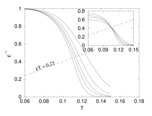
FIG. 1.: Location of the KT temperature (in dimensionless units) from MC data for the dielectric function $1/\epsilon(0)$ of the CG. System sizes are $L=6,8,10,12,16$ from top to bottom. The chemical potential is $\mu=-0.16$. Inset shows MC data corrected for finite size effects according to the text, making curves cross at $T_{c}$ given by the universal jump criterion (dashed line). The smallest system ($6\times 6$) deviates slightly and was discarded.

The main issue of this paper is to investigate the nature of the phase diagram of the 2D CG at finite vortex densities, and to compare with qualitative and quantitative features of existing theories. Figure 2 shows the phase diagram of the 2D CG for low to moderate vortex densities. The curves in the figure are various transition lines computed from our continuum simulation for the case of hard and of soft cores, lowest order equations by Kosterlitz [5], next order RG equations by Amit et al. [6] and by Timm [7], and the equations of Minnhagen [9]. All curves are KT transition lines except the low-$T$ part of the bottom curve which is a first order line; the KT part of the bottom curve extends between $T\approx 0.144$ and $T=1/4$. We see that the KT lines from all determinations coincide close to the point $(T,z)=(1/4,0)$ in the phase diagram, but otherwise they deviate significantly from each other. The agreement is expected because close to this point all theories are exact by construction, and this shows that the simulation works as expected. It is, however, clearly seen from the figure that the parameter regime in which the approximate theories give quantitative agreement is very limited.

FIG. 2.: Phase diagram of the 2D Coulomb gas. The various curves are transition lines determined by different methods (see text). Note that all curves coincide close to the point $(T,z)=(1/4,0)$ in the phase diagram, but deviate at finite $z$. The bottom curve is a KT line for $T>0.144$ and first order for $T<0.144$. All other curves are KT transition lines.

Next we will investigate the nature of the phase transition in the region of high vortex density in the phase diagram. Here different things happen for hard and soft disks: hard disk vortices have a change of ground state when the vortex core energy becomes negative from an empty system into a square vortex-antivortex crystal. Soft-core vortices instead change into a normal state where overlapping cores cover the whole system. We will here assume hard-disk vortices.

FIG. 3.: (a) Specific heat as a function of temperature $T$ at fixed chemical potentials, $\mu=0.015,0.01,\ldots,-0.02$, from left to right, for a system of hard core vortices. The system size is $20\times 20$. The curves are formed using the multiple histogram method [22] from three simulations at the parameters $T=0.0368,0.0324,0.0275$ and $\mu=0,0.005,0.01$, respectively. (b) Location of the peak in the specific heat as a function of $T$, for several system sizes.

A first indication that something changes at high densities is given in Fig. 3(a). Here we plot the specific heat as a function of temperature for a number of fixed chemical potentials. If the phase transition is of the KT type, there is no divergence in the specific heat at $T_{c}(\mu)$, but there is a peak at a somewhat higher temperature [23]. In the figure we see that, as the chemical potential is increased, the peak moves to lower temperature and gets sharper and higher, until it reaches a maximum around $T\approx 0.03$, where it starts to decrease. A possible explanation of this change of behavior would be that the KT-transition is replaced by a first order transition line at lower temperature, ending at a critical point with a diverging specific heat. Indeed the peak in the specific heat show strong finite size effects in the whole parameter region depicted in the figure. Further support of this interpretation is found using the histogram methods described below. It is difficult to give an accurate estimate of the critical exponents, since the we do not know exactly where the critical point is. Our results are, however, consistent with a value of roughly $\alpha/\nu\approx 1.6$.

The location of the peak in the specific heat for the hard core case for different fixed temperatures and system sizes forms the curves in the $(T,\mu)$-plane shown in Fig. 3(b). Close to these curves we do a more detailed analysis. We use standard histogram methods, together with a smoothing procedure described below. The procedure to locate parameter points that will extrapolate to the critical parameters in the thermodynamic limit uses histograms in two related ways. First, we use the multiple histogram method [22]. This enables us to extrapolate thermodynamic quantities to nearby values of $\mu$ and $T$, which avoids expensive simulations at every point. Secondly, we use histograms to distinguish between a continuous and a first order transition [24]. We constructed histograms using a very small bin size. This produces very noisy histograms which were then smoothed by forming averages over the 16 nearest bins. Close to a first order transition the probability distribution $P(E)$ will have a double peak structure with one peak in each phase, separated by a minimum. An example can be seen in the inset in Fig. 4. The free energy barrier between the phases is defined by $\Delta F/T=-\log(P_{max}/P_{min})$, where $P_{max}$ is the value of the probability distribution at the peak, and $P_{min}$ is at the valley in between. If the barrier increases with increasing system size this signals that there will be a first order transition in the thermodynamic limit. If it decreases there will be no phase transition, and if it is constant there will be a critical point. This analysis is usually carried out for parameters at which the two peaks have equal height. In our case, however, the histograms are highly asymmetric, which makes this criterion rather useless. Instead we use the following procedure: For a given value of the chemical potential, we adjust the temperature to the point where the two peaks have equal weight. We accomplish this by repeatedly smoothing the histogram curve by averaging over neighboring bins until the peaks become symmetric, and then we adjust $\mu$ and $T$ until their heights become equal. This method gives a practical way to approximately locate the parameters at the transition. We find that for a given $\mu$ and system size $L$, the points where the two peaks have equal weight form a curve in the $(T,\mu)$-plane, which depends slightly on the system size. In our case this curve coincides to a very good approximation with the location of the peak in the specific heat (see Fig. 3(b)), which was used as a preliminary estimate of the location of the critical parameters for each system size.

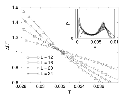
FIG. 4.: Free energy barrier $\Delta F$ determined from histograms of the Boltzmann factors in the simulation of vortices with hard cores. Inset: histograms of the Boltzmann factors $P$ vs. energy $E$ at $\mu=0.008,T\approx 0.029$. The figure shows three different behaviors: At low temperature $\Delta F$ grows with increasing system size indicating a first order transition line, ending at a critical point at $T\approx 0.032$ where all curves cross. Above this temperature the free energy barrier decreases with increasing system size. The first order line at low temperature replaces the KT transition line which starts at $T\approx 0.032$ and goes up to $T=1/4$.

Fig. 4 shows the result of the histogram analysis, for the case of hard disks. The free energy barrier $\Delta F$ was constructed from histograms of the energy distribution in the simulation. The inset shows typical such histograms of the Boltzmann factors $P$ vs. energy $E$. Three regions can clearly be seen. At low temperature, $\Delta F$ grows with increasing system size indicating a first order transition line ending at a critical point at $(T,\mu)\approx(0.032,0.004)$ where all curves cross. Above this temperature, the free energy barrier decreases with increasing system size. The first order line at low temperature replaces the KT transition line which starts at $T\approx 0.032$ and goes up to $T=1/4$. At the first order transition there is a discontinuity in the particle density, and in the energy. None of the phases have any long range positional order. For soft disks we have not found any evidence for a (finite temperature) first order transition.

Simulations on discrete lattices give qualitatively different results in the high density regime. Here one finds vortex-antivortex crystals at finite temperature and high chemical potential [13]. These phases have two distinct kinds of order: positional LRO of a staggered vorticity order parameter commensurate with the underlying discretization lattice, and finite macroscopic dielectric function. Associated with these are two separate finite temperature phase transitions: one Ising type transition and a KT transition. The Ising LRO is expected to disappear at any finite temperature in the continuum limit, when there is no pinning to an underlying lattice, but both algebraic quasi-LRO and a finite dielectric response function can in principle remain at finite $T$. To further investigate the relation between lattice and continuum simulations, and to see what happens to the phase transitions found in the lattice Coulomb gas when the continuum limit is approached, we did a sequence of lattice simulations with decreasing lattice constants.

FIG. 5.: Inverse dielectric constant from MC data on lattices with a sequence of decreasing lattice constants $a=1,\frac{1}{2},\frac{1}{4},\frac{1}{8},0$, where $a=0$ means continuum simulation. In (a) the chemical potential is negative, $\mu=-0.2$, and the KT transition temperature goes up somewhat when the lattice is removed. The system size is $16\times 16$. In (b) the chemical potential is positive, $\mu=+1.0$, and the width of the charge distribution is chosen as $r_{c}=0.1$ in units of the hard disk cutoff diameter. The system size is $8\times 8$. Here the KT transition temperature drops sharply as the discretization lattice is refined, and any finite dielectric response function of a vortex-antivortex phase is unobservable at finite temperature in the continuum case. The dashed line is the universal jump criterion for the KT-transition $\epsilon^{-1}=4T_{c}$. The crossing points give estimates of the transition temperatures for the different curves.

Figure 5 shows data for the inverse dielectric constant $1/\epsilon(0)$ for lattice constants $a=1,\frac{1}{2},\frac{1}{4},\frac{1}{8},0$, where $a=0$ means continuum simulation. In (a) the system size is $16\times 16$ and the chemical potential is negative, $\mu=-0.2$ which is in the region where the ground state is empty. We first observe that the results of the simulations interpolate smoothly from the lattice case to the continuum case as the lattice constant is decreased. This serves as a useful test that the two different Monte Carlo programs for the two cases both converge. The data in the figure imply that the KT transition temperature goes up somewhat when the discretization lattice is removed for this value of the chemical potential. To investigate why $T_{c}$ goes up when the lattice is removed, we looked at the vortex densities. For the same parameters, the lattice case has somewhat higher vortex density than the continuum case. This is because the pinning potential of the lattice favors tightly bound vortex-antivortex pairs, which leaves more space in the system for other vortices. In (b) the chemical potential is positive, $\mu=+1.0$, for which the corresponding ($T=0$) ground state is a vortex-antivortex crystal. Here the width of the charge distribution is chosen as $r_{c}=0.1$ in units of the hard disk cutoff diameter and the system size is $8\times 8$ (this choice of $r_{c}$ increases the tendency of the vortices to order in a vortex-antivortex crystal compared to our previous choice $r_{c}=\frac{1}{\sqrt{2}}e^{\gamma/2}$). Here the KT transition temperature drops sharply as the discretization lattice is refined, and any finite dielectric function of a vortex-antivortex phase is unobservable at finite temperature in the continuum case. Also the transition temperature for the Ising-Type staggered order, which for lattice constant $a=1$ is higher than the KT transition, approaches zero as the lattice constant is decreased. This demonstrates that the finite temperature crystal phases shrink down to zero temperature (or at least to smaller temperature than we could converge numerically) in the continuum limit.

V Discussion

We have constructed phase diagrams of the 2D continuum Coulomb gas from grand canonical Monte Carlo simulations, and compared it with various (approximate) analytical results (see Fig. 2). We find that all results agree at small fugacity, as expected, but at finite fugacity various results differ significantly both quantitatively and qualitatively.

We studied two different cases, namely vortices with and without an additional hard disk repulsion. In the case when the interaction is purely Coulombic we find that the transition remains continuous, consistent with the KT theory, at any negative value of the chemical potential (corresponding to fugacities $z=e^{\mu/T}<1$). At $\mu=0$ the system goes normal and the CG model breaks down. On the other hand, when a hard core repulsive interaction is added to the Coulomb interaction, we find evidence from finite size scaling of the Monte Carlo data for a first order transition at finite but low temperature, $T\lesssim 0.032$, and at a small positive value of the chemical potential. Our critical endpoint $T\approx 0.032$ is roughly consistent with the one found in Ref. [15]. We do not find first order transitions at negative chemical potentials as in Refs. [9, 11].

The existence of our first order transition is related to the change of ground state at the point where the chemical potential exceeds the Coulomb energy per particle in a square vortex-antivortex lattice, with lattice constant equal to the hard disk diameter. This energy should be compared to the basic energy scale for creating vortices, the pair creation energy, which is the total energy of a vortex-antivortex pair whose hard disks touch. Both the crystallization energy and the pair creation energy depend very strongly on the ratio between the hard disk diameter and the short distance cutoff, $r_{c}$, in the Coulomb interaction. Indeed we find that, in all cases we tried, the value of $\mu$ at which the first order transition takes place is slightly above the ground state crystalization energy (but below the pair creation energy). It is interesting to note, however, that this finite temperature first order transition takes place not between the empty state and the vortex-antivortex crystal, but between a gas-like low density phase and a liquid-like high density phase, with no long range order. This is in contrast with simulations done on an underlying discretization lattice, where the first order transition is to a vortex-antivortex crystal [13].

To investigate this effect further we did a sequence of lattice simulations with different lattice constants, $a=1,\frac{1}{2},\frac{1}{4},\frac{1}{8},0$. We find that the extent of the LRO vortex-antivortex crystal phase shrink rapidly towards zero temperature with decreasing lattice constant, leaving no sign in the continuum case, at least for the parameters considered by us. We can, however, not rule out the possibility of quasi-LRO, orientational order, etc., at lower temperatures than could be safely converged in our simulations. It should be mentioned that in this parameter regime (high density, low temperature) it is very hard to converge the simulations, and all our results are for rather small systems due to limitations in what sizes we are able to converge safely.

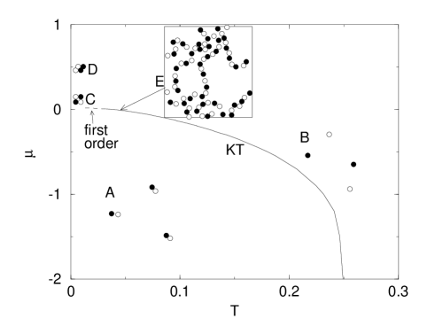
FIG. 6.: Phase diagram with snapshots of typical configurations inserted. The displayed snapshots are the following: (A) superfluid vortex-dipole phase at low density. (B) non-superfluid free vortex phase. (C) square vortex-antivortex crystal ground state at small positive vortex chemical potential (negative core energy). (D) triangular (frustrated) vortex crystal above some threshold value of the chemical potential. (E) characteristic 1D vortex-antivortex patterns in the regime where the dense vortex liquid evaporates.

To summarize our results, we will now discuss several qualitative features of the phase diagram of the 2D CG with hard disks. Figure 6 shows the phase diagram in the $(T,\mu)$-plane together with several snapshots of typical vortex configurations obtained in our simulations. Below the KT transition line the system is in a superfluid phase where all vortices present in the system are bound together in pairs of opposite vorticity. In this phase the vortex-vortex correlation function decays algebraically so there is no LRO, but nevertheless the long distance macroscopic dielectric function $\epsilon$ is finite, corresponding to a phase with finite macroscopic superfluid density. Above the KT transition, free vortices appear and the macroscopic superfluidity is destroyed. Our simulation shows that this happens at any choice of the chemical potential as long as it is negative. In Fig. 6, the KT transition line extends some (small) distance into the region of positive chemical potential, and is then taken over by a first order transition line at low temperature and small positive chemical potential.

Our simulations are at finite temperature, but at zero temperature we have the following three distinct ground states: an empty system (no vortices) at low vortex chemical potential, a square vortex-antivortex crystal above a certain chemical potential, which is always positive, and a close-packed triangular (frustrated) vortex crystal above a second threshold value of the chemical potential. The crystal states are indicated schematically in Fig. 6. We simulated down to low, but finite temperatures, but did not reach low enough to observe any traces of these crystal states. We can therefore not decide if crystalline order, with finite dielectric response function, remains at small but non-zero temperatures. Long range crystal order can also be destroyed at zero temperature by quantum melting, which is not included in our classical model. However, instead of crystalline LRO, we find the typical short range positional correlations shown in the inset in Fig. 6, close to the region of the first order transition. There are tendencies to form both 2D vortex-antivortex finite clusters and also characteristic 1D vortex-antivortex strings appear. The configurations are strongly fluctuating, with strong density fluctuations, and a snapshot at a later time will look very different but with the same kind of typical positional correlations.

Qualitatively different phase diagrams containing vortex-antivortex crystal states have been discussed in the literature. We do not observe the thermally created vortex-antivortex crystals in superfluids/superconductors that were proposed in Refs [25, 26].

Finally we will discuss the possible experimental consequences of our phase diagram. In the usual applications, like superfluid and superconducting films, where the only vortices present are due to thermal fluctuations (i.e. at negative vortex chemical potential), our simulations show that there will always be a KT transition. According to our results, first order transitions can happen only when the creation energy for a vortex pair is negative, i.e., for positive chemical potential. To enter this parameter regime it is necessary to have a short range repulsion between the vortices, such as in the hard disk model. We expect that this is not usually the case in superconducting or superfluid films, but it should not be excluded that quantum fluctuations could effectively lead to this situation in peculiar cases. In any case our simulation shows that a KT transition is not the only possibility in this parameter regime. An example of a physical system, which has many of the properties of our CG model in the parameter regime where we predict first order transitions, is provided by spin textures in quantum Hall systems. In double layer quantum Hall systems at the filled lowest Landau level, i.e. one flux quantum of the perpendicular magnetic field penetrates the sample for each electron in the 2D electron gas, a finite temperature KT transition has been predicted [4], and studied by lattice simulations [27]. Away in filling from the filled Landau level there will be extra charges or holes present. There is a certain regime where the excess charge cause the formation of electrically charged pseudospin vortices [4], such that each vortex carries electric charge $\pm e/2$. This system thus automatically has a finite density of vortex-antivortex pairs also at low temperature, so at low enough temperature the vortex chemical potential is positive. Furthermore, the hard disks correspond very roughly to the Coulomb repulsion between the electric charges. Thus the basic requirements for observing our first order transitions are fulfilled, but clearly a more detailed analysis taking into account for example the long range nature of the electric Coulomb repulsion is needed. This motivates further simulations of this physical system using more realistic models.

We thank Steve Girvin, Kenneth Holmlund, Edwin Langmann, Petter Minnhagen, Peter Olsson, and Hans Weber for valuable discussions. This work was supported by the Swedish Natural Science Research Council.

REFERENCES

- [1] V.L. Berezinskii, Zh. Eksp. Teor. Fiz. 61, 1144 (1971) [Sov. Phys. JETP 34, 610 (1972)]. J.M. Kosterlitz and D.J. Thouless, J. Phys. C 5, L124 (1972); ibid 6, 1181 (1973).
- [2] P. Minnhagen, Rev. Mod. Phys. 59, 1001 (1987).
- [3] B. Nienhuis, in Phase Transitions and Critical Phenomena, edited by C. Domb and J.L. Lebowitz (Academic, New York, 1987), Vol. 11.
- [4] K. Yang, K. Moon, L. Zheng, A.H. MacDonald, S.M. Girvin, D. Yoshioka, and S.-C. Zhang, Phys. Rev. Lett. 72, 732 (1994). K. Moon, H. Mori, K. Yang, S.M. Girvin, A.H. MacDonald, L. Zheng, D. Yoshioka, and S.-C. Zhang, Phys. Rev. B 51, 5138 (1995).
- [5] J.M. Kosterlitz, J. Phys. C 7, 1046 (1974).
- [6] D.J. Amit, Y.Y. Goldschmidt, and G. Grinstein, J. Phys. A 13, 585. (1980)
- [7] C. Timm, preprint cond-mat/9602124.
- [8] P. Minnhagen, Phys. Rev. Lett. 54, 2351 (1985); Phys. Rev. B 32, 3088 (1985).
- [9] P. Minnhagen and M. Wallin, Phys. Rev. B 36, 5620 (1987); ibid. 40, 5109 (1989).
- [10] J.M. Thijssen and H.J.F. Knops, Phys. Rev. B 38, 9080 (1988).
- [11] G.-M. Zhang, H. Chen and X. Wu, Phys. Rev. B 48, 12304 (1993); B.-W. Xu and Y.-M. Zhang, Phys. Rev. B 50 18651 (1994); G.-M. Ding and B.-W. Xu, Phys. Rev. B 51 12653 (1995).
- [12] Y. Levin, X. Li, and M.E. Fisher, Phys. Rev. Lett. 73, 2716 (1994).
- [13] J.-R. Lee and S. Teitel, Phys. Rev. Lett. 64, 1483 (1990); Phys. Rev. B 46, 3247 (1992).
- [14] J.M. Caillol and D. Levesque, Phys. Rev. B 33, 499 (1986).
- [15] G. Orkoulas and A.Z. Panagiotopoulos, J. Chem. Phys. 104, 7205 (1996).
- [16] K. Holmlund and P. Minnhagen, (unpublished).
- [17] D.R. Nelson and J.M. Kosterlitz, Phys. Rev. Lett. 39, 1201 (1977). T. Ohta and D. Jasnow, Phys. Rev. B 20, 130 (1979). P. Minnhagen and G.G. Warren, Phys. Rev. B 24, 2526 (1981).
- [18] P. Olsson, Phys. Rev. B 52, 4511 (1995).
- [19] A. Vallat and H. Beck, Phys. Rev. B 50, 4015 (1994).
- [20] H. Weber and P. Minnhagen, Phys. Rev. B 37, 5986 (1988).
- [21] J.P. Valleau and L.K. Cohen, J. Chem. Phys. 72, 5935 (1980).
- [22] A.M. Ferrenberg and R.H. Swendsen, Phys. Rev. Lett. 61, 2635 (1988); 63, 1195 (1989).
- [23] M.N. Barber, in Phase Transitions and Critical Phenomena, edited by C. Domb and J.L. Lebowitz (Academic, New York, 1983), Vol. 8.
- [24] J. Lee and J.M. Kosterlitz, Phys. Rev. Lett. 65, 137 (1990); Phys. Rev. B 43, 1268 (1991); 43, 3265 (1991).
- [25] M. Gabay and A. Kapitulnik, Phys. Rev. Lett. 71, 2138 (1993).
- [26] S.-C. Zhang, Phys. Rev. Lett. 71, 2142 (1993).
- [27] I. Tupitsyn, M. Wallin, and A. Rosengren, Phys. Rev. B 53, R7614 (1996).