[

Velocity Selection for Propagating Fronts in Superconductors

Abstract

Using the time-dependent Ginzburg-Landau equations we study the propagation of planar fronts in superconductors, which would appear after a quench to zero applied magnetic field. Our numerical solutions show that the fronts propagate at a unique speed which is controlled by the amount of magnetic flux trapped in the front. For small flux the speed can be determined from the linear marginal stability hypothesis, while for large flux the speed may be calculated using matched asymptotic expansions. At a special point the order parameter and vector potential are dual, leading to an exact solution which is used as the starting point for a perturbative analysis.

]

There exists a wide class of problems in which a system, subjected to a sudden destabilizing change, responds by forming fronts which propagate into the unstable state. This phenomena occurs in models of population dynamics [3, 4, 5], pulse propagation [6], liquid crystals [7], solidification [8], and tubular vesicles [9]; further examples are discussed in Ref. [10]. The interesting issues common to all of these problems are whether the fronts approach a constant, unique speed, and if so, how the system selects this speed out of a manifold of possible speeds. The prototype is Fisher’s equation [3, 4],

$$\partial_{t}u=\partial^{2}_{x}u+F(u),$$ (1)

where $u>0$ may be interpreted as a population density, and $F(0)=F(1)=0$. As shown rigorously by Aronson and Weinberger [5], for a sufficiently localized initial condition the solutions of this equation evolve into fronts of the form $u(x,t)=U(x-ct)$ which connect $u=1$ at $x=-\infty$ to $u=0$ at $x=\infty$; the speed of the front satisfies $2\sqrt{F^{\prime}(0)}\leq c\leq 2\ {\rm sup}\sqrt{F(u)/u}$, so that for the special case $F(u)=u-u^{3}$ the selected speed is $c=2$. There have been many attempts to generalize these results to more complicated equations and physical systems, including heuristic methods such as the marginal stability hypothesis (MSH) [11, 12] and the structural stability hypothesis [13, 14], construction of exact solutions [12, 15], variational methods [14, 16, 17], and dynamical systems methods [18].

In this paper we will study a closely related problem of front (or interface) propagation in superconductors. The problem which we have in mind is the following: begin with a bulk superconductor in an applied magnetic field equal to the critical field $H_{c}$, so that there is a stationary, planar superconducting-normal interface which separates the normal and superconducting phases; then rapidly reduce the applied field to zero, so that the now unstable interface propagates toward the normal phase so as to expel any trapped magnetic flux, leaving the sample in the Meissner phase. Assuming that the interface remains planar, what is its dynamics? In this paper we will show that under these conditions constant velocity fronts do propagate, at a unique speed which is controlled by the amount of magnetic flux which is trapped in the front [19]. We calculate this speed in different parameter regimes using the MSH, a perturbative calculation about an exact solution which we have discovered, and an asymptotic analysis valid for small speeds. Where appropriate, our analytic results are compared to extensive numerical solutions of the dynamic equations.

To analyze the behavior of the superconducting-normal boundary, we use the one-dimensional time-dependent Ginzburg-Landau (TDGL) equations, which in dimensionless units [20] are

$$\partial_{t}f={1\over\kappa^{2}}\partial^{2}_{x}f-q^{2}f+f-f^{3},$$ (2)

$$\bar{\sigma}\partial_{t}q=\partial^{2}_{x}q-f^{2}q,$$ (3)

where $f$ is the magnitude of the superconducting order parameter, $q$ is the gauge-invariant vector potential (such that $h=\partial_{x}q$ is the magnetic field), $\kappa$ is the Ginzburg-Landau parameter, and $\bar{\sigma}$ is the dimensionless normal state conductivity (the ratio of the order parameter diffusion constant to the magnetic field diffusion constant). Notice that if the vector potential is zero, then Eq. (2) is exactly Fisher’s equation, Eq. (1), with fronts which propagate at a speed $c=2/\kappa$ in our units. Since lengths are measured in units of the penetration depth (typically of order 500 Å in type-I superconductors) and time in units of the order parameter relaxation time (of order $10^{-9}$–$10^{-10}$ s), the characteristic scale for speeds is of order 100 m/s [21]. For the propagating solutions which we are considering (i.e., after the field quench), $f=1$, $q=0$, and $h=0$ as $x\rightarrow-\infty$ (the superconducting phase), and $f=0$, $q=Q_{\infty}$, and $h=0$ as $x\rightarrow\infty$ (the normal phase). The physical meaning of $Q_{\infty}$ is clear once we notice that the integrated magnetic field in the front (i.e., the total magnetic flux per unit length parallel to the front) is $\int_{-\infty}^{\infty}h(x)\,dx=Q_{\infty}$. As we will see, $Q_{\infty}$ is an important control parameter for the front dynamics—the larger the trapped magnetic flux in the front the smaller the front speed.

We have solved Eqs. (2) and (3) numerically for a wide range of $\kappa$, $\bar{\sigma}$ and $Q_{\infty}$, using the Crank-Nicholson method [22]. An initial configuration for the order parameter and magnetic field with the appropriate boundary conditions is established and then allowed to evolve in time. For our boundary conditions (in particular, $h=0$ as $x\rightarrow\infty$), the front rapidly approaches a constant velocity. On an IBM RS 6000/370 approximately 5000 cpu minutes are needed to trace this evolution (allowing 300-500 time units to elapse usually brings us sufficiently close to a constant velocity solution). We analyze the profile of the order parameter and magnetic field for the constant velocity solutions (see Fig. 1 for a representative result) and determine the value of the front velocity as a function of $Q_{\infty}$, as shown in Fig. 2. The remainder of this paper is devoted to an analysis of the TDGL equations which will shed some light on these numerical results.

To begin our analysis we will search for steady traveling wave solutions of the TDGL equations, of the form $f(x,t)=F(X)$ and $q(x,t)=Q(X)$ where $X=x-ct$ with $c>0$. Then the TDGL equations become

$${1\over\kappa^{2}}F^{\prime\prime}+cF^{\prime}-Q^{2}F+F-F^{3}=0,$$ (4)

$$Q^{\prime\prime}+\bar{\sigma}cQ^{\prime}-F^{2}Q=0,$$ (5)

(the primes denote differentiation with respect to $X$). The order parameter connects $F=1$ at $X=-\infty$ to $F=0$ at $X=\infty$, while the vector potential connects $Q=0$ at $X=-\infty$ to $Q=Q_{\infty}$ at $X=\infty$. In the spirit of the MSH, we first examine the linear stability of the leading edge of the front ($X\rightarrow\infty$). Linearizing Eqs. (4)

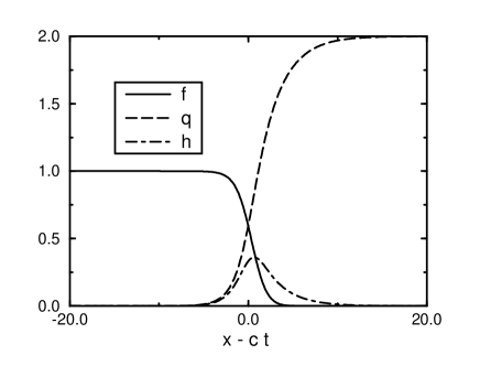
FIG. 1.: Numerical solution for $\kappa=1$, $\bar{\sigma}=1$, and $Q_{\infty}=2$, resulting in a front which moves to the right with speed $c=0.386$. Shown are the order parameter (solid line), vector potential (dashed line), and field (dashed-dotted line).

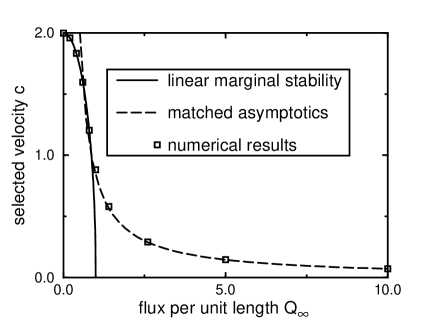
FIG. 2.: Numerical values (open squares) of the front speed as a function of $Q_{\infty}$ for $\kappa=1$ and $\bar{\sigma}=1$. Also shown are the results of the linear marginal stability analysis (solid line) and matched asymptotic analysis (dashed line).

and (5), we find $F(X)\sim\exp(-\lambda_{-}X)$, with

$$\lambda_{-}={c\kappa^{2}\over 2}-\sqrt{\left({c\kappa^{2}\over 2}\right)^{2}-\kappa^{2}[1-Q_{\infty}^{2}]}.$$ (6)

Since the magnitude of the order parameter $F\geq 0$, we require ${\rm Im}(\lambda_{-})=0$ in order to prevent the solution from oscillating, which implies

$$c\geq c^{\prime}={2\sqrt{1-Q_{\infty}^{2}}\over\kappa}\qquad(Q_{\infty}\leq 1),$$ (7)

with $c\geq 0$ for $Q_{\infty}\geq 1$. In addition to this lower bound on the speed, we conjecture that $c\leq 2/\kappa$, since we expect the front to have the greatest speed in the absence of any trapped flux. The MSH [11, 12] would have us set $c=c^{\prime}$; at this speed the leading edge of the order parameter front is marginally stable with respect to perturbations—the phase and group velocities of the perturbation are equal at this speed. At $Q_{\infty}=0$, this yields $c=2/\kappa$, which is the rigorous result for Fisher’s equation [4, 5]. In Fig. 2 we compare the result of the MSH against the numerical results. We see that for small $Q_{\infty}$ there is a close agreement between the numerics and the MSH result. However, as $Q_{\infty}$ approaches 1 we begin to see significant departures from the MSH; the MSH predicts that the front should be stationary for $Q_{\infty}>1$. We therefore see that the linear MSH fails to accurately predict the selected front speed for sufficiently large trapped flux.

Further understanding of the selection problem can be gleaned from an exact solution of the TDGL equations for $Q_{\infty}=1$, $\kappa=1/\sqrt{2}$, and $\bar{\sigma}=1/2$. To motivate this solution, we first notice that when $Q_{\infty}=1$, it appears qualitatively that $F+Q=1$. With this in mind, we look for solutions to (4) and (5) of the form $F(X)=1-Q(X)$; by substituting this Ansatz into (4) and (5), we find that this is only consistent when $\kappa=1/\sqrt{2}$ and $\bar{\sigma}=1/2$. For this set of parameters the equation for the order parameter reduces to

$$F^{\prime\prime}+{c\over 2}F^{\prime}+F^{2}-F^{3}=0.$$ (8)

The exact solution of Eq. (8) can be constructed using the reduction of order method described by van Saarloos (see Ref. [12], Sec. IV), with the result that $c=\sqrt{2}$, and the order parameter and vector potential are (up to translations)

$$F(X)={1\over e^{X/\sqrt{2}}+1},\quad Q(X)={1\over e^{-X/\sqrt{2}}+1}.$$ (9)

It should be emphasized that this duality between $F$ and $Q$ is distinct from the well known duality between the order parameter and the magnetic field which exists in the equilibrium Ginzburg-Landau (GL) equations at $\kappa=1/\sqrt{2}$ [23]. To the best of our knowledge this is the only known exact solution of the TDGL equations.

The exact solution serves as a useful check on our numerical results; our numerical solution of (2) and (3) for this set of parameters gives $c=1.4142$, bolstering confidence in the numerical work. The exact solution also illustrates the limitations of the linear MSH, which predicts a speed of $c=0$ for these parameters. Finally, the exact solution can also serve as the starting point for perturbative solutions of the TDGL equations, along the lines of the renormalization group method discussed in Ref. [14]. We find [24]

$$c=\sqrt{2}\left[1-\frac{1}{6}\epsilon_{\kappa}-\frac{2}{3}\epsilon_{\sigma}-\epsilon_{Q}+O(\epsilon^{2})\right],$$ (10)

with $\epsilon_{\kappa}=2-1/\kappa^{2}$, $\epsilon_{\sigma}=\sigma-1/2$, and $\epsilon_{Q}=Q_{\infty}-1$. For example, when $\kappa=0.6$, $\sigma=0.5$, and $Q_{\infty}=1$, Eq. (10) yields $c=1.5975$, while the numerical result is $c=1.5826$.

Although the exact solution described above is a useful touchstone for our numerical work, we desire a more general approach to the problem of calculating the front speed. To do this we develop a perturbative solution of Eqs. (4) and (5) for small $c$ (large trapped flux); a similar treatment for curved interfaces in two dimensions has been given in Refs. [20] and [25]. Expand the solutions in powers of $c$ (the inner expansion),

$$F(X;c) = F_{0}(X)+cF_{1}(X)+\ldots,$$ (11)

$$Q(X;c) = Q_{0}(X)+cQ_{1}(X)+\ldots\ ,$$ (12)

and substitute these expansions into Eqs. (4) and (5). The $O(1)$ equations for $(F_{0},Q_{0})$ are the GL equations. The important feature of the solutions for our purposes is that the vector potential in the normal phase ($X\rightarrow\infty$) has the asymptotic behavior (up to a translation)

$$Q_{0}(X)\sim{X\over\sqrt{2}}+{\rm e.s.t.},$$ (13)

where e.s.t.=“exponentially small terms.” This result shows that the magnetic field in the normal phase approaches $1/\sqrt{2}$ (which is $H_{c}$ in conventional units)—a planar interface can only be in equilibrium when the field in the normal phase is $H_{c}$. Proceeding to $O(c)$, we have

$${1\over\kappa^{2}}F_{1}^{\prime\prime} - (Q_{0})^{2}F_{1}-2Q_{0}F_{0}Q_{1}$$ (15)

$$+[1-3(F_{0})^{2}]F_{1}=-F_{0}^{\prime},$$

$$Q_{1}^{\prime\prime}-(F_{0})^{2}Q_{1}-2F_{0}Q_{0}F_{1}=-\bar{\sigma}Q_{0}^{\prime}.$$ (16)

The asymptotic behavior of $Q_{1}$ can be obtained as follows. Multiply Eq. (15) by $F_{0}^{\prime}$, Eq. (16) by $Q_{0}^{\prime}$, add the two equations together, and integrate the result from $-\infty$ to $X$. Then integrate $F_{1}^{\prime\prime}$ and $Q_{1}^{\prime\prime}$ by parts twice, and use the fact that $(F_{0}^{\prime},Q_{0}^{\prime})$ are solutions to the homogeneous versions of Eqs. (15) and (16) (the zero mode). The final result for the asymptotic behavior as $X\rightarrow\infty$ is

$$Q_{1}(X)\sim-{\bar{\sigma}\over 2\sqrt{2}}X^{2}-{\beta\over\sqrt{2}}X+C_{1}+{\rm e.s.t.},$$ (17)

where $C_{1}$ is an integration constant and $\beta$ is given by

$$\beta=2\int_{-\infty}^{\infty}\left[(F_{0}^{\prime})^{2}+\bar{\sigma}(Q_{0}^{\prime})^{2}-{\bar{\sigma}\over\sqrt{2}}Q_{0}^{\prime}\right]dx.$$ (18)

The kinetic coefficient $\beta(\kappa,\bar{\sigma})$ must be determined numerically from the solutions of the GL equations [26].

By comparing $Q_{0}$ and $cQ_{1}$, we see that these two terms become comparable when $cX=O(1)$, indicating a breakdown of the perturbative expansion. This suggests introducing the outer variable $\xi=cX$, with $f(\xi)=F(X)$ and $q(\xi)=Q(X)$. In terms of these outer variables Eqs. (4) and (5) become

$${c^{2}\over\kappa^{2}}f^{\prime\prime}+c^{2}f^{\prime}-q^{2}f+f-f^{3}=0,$$ (19)

$$c^{2}q^{\prime\prime}+\bar{\sigma}c^{2}q^{\prime}-f^{2}q=0.$$ (20)

Expanding the solutions in powers of $c$,

$$f(\xi;c) = f_{0}(\xi)+cf_{1}(\xi)+\ldots,$$ (21)

$$q(\xi;c) = {q_{0}(\xi)\over c}+q_{1}(\xi)+\ldots$$ (22)

we find that $f_{0}=1$, $f_{1}=0$ in the outer superconducting region ($\xi\rightarrow-\infty$), $f_{0}=f_{1}=0$ in the outer normal region ($\xi\rightarrow\infty$), and $q_{0}=q_{1}=0$ in the outer superconducting region, with

$$q_{0}(\xi)=A_{0}+B_{0}e^{-\bar{\sigma}\xi},\quad q_{1}(\xi)=A_{1}+B_{1}e^{-\bar{\sigma}\xi}$$ (23)

in the outer normal regions; $A_{n}$ and $B_{n}$ are integration constants. The inner and outer solutions must now be matched together in an appropriate overlap region [20, 25], with the result

$$A_{0}=-B_{0}={1\over\sqrt{2}\bar{\sigma}},\quad A_{1}=-B_{1}=-{\beta\over\sqrt{2}\bar{\sigma}}.$$ (24)

Using this expansion, we can determine the asymptotic value of the vector potential in the normal phase as an expansion in powers of $c$:

$$Q_{\infty}={1\over\sqrt{2}\bar{\sigma}c}-{\beta\over\sqrt{2}\bar{\sigma}}+O(c).$$ (25)

If we think of $Q_{\infty}$ as the control variable, then we have for the selected velocity

$$c={1\over\sqrt{2}\bar{\sigma}Q_{\infty}+\beta}.$$ (26)

As was pointed out in [20, 25, 26] the kinetic coefficient may actually be negative for some values of the parameters. One might worry that when $\sqrt{2}\bar{\sigma}Q_{\infty}=-\beta$, Eq. (26) predicts an infinite velocity, contradicting our conjecture that $c\leq 2/\kappa$. However, if this occurs we simply have a breakdown of the perturbation expansion, indicating the need to keep higher order terms. In Fig. 2 we compare the asymptotic result, Eq. (26), and the numerical results, for $\kappa=1$ and $\bar{\sigma}=1$; the kinetic coefficient for these parameters is $\beta=-0.216$ [26]. The agreement is excellent in the appropriate region of large $Q_{\infty}$. The agreement is equally impressive for other values of $\kappa$ and $\bar{\sigma}$. In particular, when $\kappa=1/\sqrt{2}$ and $\bar{\sigma}=1/2$, $\beta=0$ [20], so that the asymptotic analysis predicts $c=\sqrt{2}/Q_{\infty}$; if we set $Q_{\infty}=1+\epsilon_{Q}$, and expand for small $\epsilon_{Q}$, then $c=\sqrt{2}[1-\epsilon_{Q}+O(\epsilon^{2})]$, which agrees to lowest order with the expansion about the exact result given in Eq. (10).

In summary, we have studied the propagation of fronts separating the superconducting and normal phases, which are produced after a quench to zero applied magnetic field. In addition to its possible practical importance in understanding flux expulsion in superconductors, this problem provides an interesting variation on the theme of front propagation in unstable systems. By varying the amount of flux trapped in the front we can go continuously from a regime at small flux in which the speed is close to that predicted by the linear marginal stability hypothesis, to a regime at high flux which can be treated using the method of matched asymptotic expansions. While we have no general results at intermediate values of the flux, for a particular set of parameters we have discovered an exact solution, which serves as the starting point for a perturbative calculation in this regime. We are currently expanding our study to include front propagation in two dimensions and a detailed study of the diffusive fronts which appear after quenches to non-zero applied fields [24].

We would like to thank R. E. Goldstein and M. Fowler for helpful discussions. This work was supported by NSF Grants DMR 92-23586 and 96-28926.

REFERENCES

- [1] Electronic address: sjd2u@virginia.edu
- [2] Electronic address: atd2h@virginia.edu
- [3] R. A. Fisher, Ann. Eugen. 7, 355 (1937).
- [4] A. N. Kolmogorov, I. G. Petrovskii, and N. S. Piskunov, Bull. Univ. Moscow, Ser. Int. A 1, 1 (1937).
- [5] D. G. Aronson and H. F. Weinberger, Adv. Math. 30, 33 (1978).
- [6] A. C. Scott, Neurophysics (Wiley, New York, 1977).
- [7] W. van Saarloos, M. van Hecke, and R. Holyst, Phys. Rev. E 52, 1773 (1995).
- [8] H. Löwen and J. Bechhoefer, Europhys. Lett. 16, 195 (1991); A. A. Wheeler, W. J. Boettinger, and G. B. McFadden, Phys. Rev. A 45, 7424 (1992); R. Kupferman et al., Phys. Rev. B 46, 16 045 (1992); M. N. Barber and D. Singleton, J. Austral. Math. Soc. B 36, 325 (1994).
- [9] R. E. Goldstein et al., J. Phys. II (France) 6, 767 (1996).
- [10] M. C. Cross and P. C. Hohenberg, Rev. Mod. Phys. 65, 851 (1993).
- [11] E. Ben-Jacob et al., Physica D 14, 348 (1985).
- [12] W. van Saarloos, Phys. Rev. B 39, 6367 (1989).
- [13] G. C. Paquette et al., Phys. Rev. Lett. 72, 76 (1994).
- [14] L.-Y. Chen, N. D. Goldenfeld, and Y. Oono, Phys. Rev. E 49, 4502 (1994).
- [15] R. D. Benguria and M. C. Depassier, Phys. Rev. E 50, 3701 (1994).
- [16] R. D. Benguria and M. C. Depassier, Phys. Rev. Lett. 73, 2272 (1994).
- [17] R. D. Benguria and M. C. Depassier, Commun. Math. Phys. 175, 221 (1996).
- [18] A. Goriely, Phys. Rev. Lett. 75, 2047 (1995).
- [19] This should be contrasted with previous work which considered a quench to a non-zero applied field, where the interface moves diffusively; see H. Frahm, S. Ullah, and A. T. Dorsey, Phys. Rev. Lett. 66, 3067 (1991); F. Liu, M. Mondello, and N. D. Goldenfeld, Phys. Rev. Lett. 66, 3071 (1991).
- [20] A. T. Dorsey, Ann. Phys. 233, 248 (1994).
- [21] While it might appear to be difficult to observe fronts with these speeds, they are actually well within the capability of high speed magneto-optic methods; see P. Leiderer et al., Phys. Rev. Lett. 71, 2646 (1993).
- [22] W. H. Press, S. A. Teukolsky, W. T. Vetterling, and B. P. Flannery, Numerical Recipes in FORTRAN, Second Edition (Cambridge University Press, Cambridge, UK, 1992), Ch. 19.
- [23] D. Saint-James, G. Sarma, and E. J. Thomas, Type-II Superconductivity (Pergamon Press, Oxford, 1969), p. 36; E. B. Bogomol’nyi, Sov. J. Nucl. Phys. 24, 449 (1977).
- [24] S. J. Di Bartolo and A. T. Dorsey (unpublished).
- [25] S. J. Chapman, Quart. J. Appl. Math. 53, 601 (1995).
- [26] J. C. Osborn and A. T. Dorsey, Phys. Rev. B 50, 15 961 (1994); defined in the present paper is the same as .