A class of ansatz wave functions for 1D spin systems and their relation to DMRG

Abstract

We investigate the density matrix renormalization group (DMRG) discovered by White and show that in the case where the renormalization eventually converges to a fixed point the DMRG ground state can be simply written as a “matrix product” form. This ground state can also be rederived through a simple variational ansatz making no reference to the DMRG construction. We also show how to construct the “matrix product” states and how to calculate their properties, including the excitation spectrum. This paper provides details of many results announced in an earlier letter.

I Introduction

After Wilson’s development of the renormalization group (RG) to solve the Kondo problem [1] it was believed that RG could be used for other problems as well. Kadanoff’s blocking technique combined with Wilson’s RG idea was applied to problems like quantum lattice systems such as the Hubbard and Heisenberg models but progress turned out to be surprisingly difficult. However, in 1992 White developed the density matrix renormalization group (DMRG) [2, 3] method which since then has had a spectacular success in calculating ground state energies and other static properties of many 1D quantum systems. In this paper we explore the nature and underlying principles of the DMRG to find out why the results of DMRG calculations are so remarkable accurate. A summary of this work has been presented in an earlier paper [4], and the present paper provides a complete discussion and derivations of the results. For background information on the DMRG there are excellent articles by White [2, 3].

In Sec. II we give a very brief summary of the DMRG. In Sec. III we show that if the DMRG algorithm converges to a fixed point, the DMRG ground state leads to a special ansatz form for the wave function, demonstrating the equivalence of the DMRG to a variational calculation. To make things more concrete we apply our ideas to the antiferromagnetic Heisenberg spin-1 chain with quadratic and biquadratic interactions, defined by

$$H=\sum_{i=1}^{n}{\bf S}_{i}\cdot{\bf S}_{i+1}-\beta({\bf S}_{i}\cdot{\bf S}_{i+1})^{2}.$$ (1)

In Sec. IV we define a set of variational states using the special ansatz form of Sec. III. In Sec. V we extend the ansatz to include a set of Bloch states that describe elementary excitations in both finite and infinite systems. These calculations are rather lengthy and the details can be found in appendices. Sec. VI contains some numerical results for the spin-1 chain to compare our variational ansatz to more involved calculations.

We would like to mention that all numerical work described here was programmed with Mathematica on an ordinary desktop workstation. Each calculation we describe here take anywhere from a few seconds to a few minutes.

II Density Matrix Renormalization Group (DMRG)

Since the DMRG was discovered by S.R. White [2] in 1992 it has had great success in describing 1D interacting quantum systems [3, 5, 6, 7]. Ground state and excited state properties have been calculated to high accuracy with modest computational effort. With hindsight, it will be seen that the ideas of this paper do not logically depend on the DMRG, but they were inspired by the DMRG and we will therefore begin this section by summarizing some aspects of the DMRG.

In a renormalization scheme like the DMRG one typically starts with a very short 1D chain and then lets the length increase by iteratively adding a single site. After each new site, an approximate Hamiltonian is constructed. This is done by keeping only a small subspace of the Hilbert space to keep the Hilbert space at a manageable size as one lets the chain grow. The central idea in DMRG is to keep the “most probable” states when truncating the basis in contrast to the usual old-fashioned real space RG methods (see e.g. Ref. [3] and references therein) where the lowest energy eigenstates are kept. The way to achieve this is to split a complete system (“universe”) into two parts, a “subsystem” and an “environment” and then to construct the reduced density matrix for the “subsystem” as part of the “universe”. The state of the “subsystem” is then given by a linear combination of the eigenstates of the density matrix with weights given by the eigenvalues.

The renormalization starts with a short 1D lattice with just a few sites. Label this system $H_{B}$. A renormalization step of the DMRG can be described by the following algorithm:

1. Construct the Hamiltonian for the “universe”, $H_{S}=H_{B}+H_{1}+H_{1}^{R}+H_{B}^{R}$, where $H_{B}$ comes from the previous iteration and $H_{1}$ is a new site added. The superscript $R$ denotes a second block that is reflected before joined to the other parts. The block $H_{B}+H_{1}$ now is our “subsystem” and $H_{1}^{R}+H_{B}^{R}$ our “environment”. The Hamiltonian matrix $H_{S}$ for the “universe” is constructed with tensor products involving the intrablock parts $H_{B}$ and $H_{1}$ and the interactions between the blocks.

2. Diagonalize $H_{S}$ to obtain the ground state $|\Psi\rangle$ of the “universe”. This state is called the target state.

3. Construct the reduced density matrix $\rho_{i,i^{\prime}}=\sum_{j}\Psi_{i,j}\Psi^{*}_{i^{\prime},j}$, where $|\Psi\rangle=\sum_{i,j}\Psi_{i,j}|i\rangle\otimes|j\rangle$ and $|i\rangle,|j\rangle$ are basis states of the “subsystem” and the “environment” respectively. The eigenstates of $\rho$ with the highest eigenvalues correspond to the most probable states of the “subsystem” when the “universe” is in the state $|\Psi\rangle$.

4. Now choose the $m$ states of the diagonalized density matrix with highest eigenvalues to form a new reduced basis for the block $H_{B}+H_{1}$ . Project the Hamiltonian and other operators onto this basis by $H_{B^{\prime}}=A(H_{B+1})A^{\dagger}$, where $A$ is the projection operator one constructs from the kept eigenstates of the density matrix from step 3 and $H_{B+1}$ is the Hamiltonian matrix for the “subsystem”. If the single site added has $m_{s}$ states in its basis, $A$ is represented by a $m\times(m*m_{s})$ matrix and $H_{B+1}$ by a $(m*m_{s})\times(m*m_{s})$ matrix.

5. Rename $H_{B^{\prime}}$ to $H_{B}$.

This completes an iteration.

III The matrix product state

To begin the renormalization procedure one starts with a block consisting of a short lattice whose basis states can be calculated exactly. When the renormalization proceeds and the chain described by the block gets longer we don’t use the full set of basis states for describing the block but have to discard some part of the Hilbert space in each renormalization step.

Assume we have a block that represents a chain with $n-1$ sites. Let $m_{s}$ be the number of possible states of a singe lattice site. If we would treat this system exactly there would be $m_{s}^{n-1}$ states in the Hilbert space basis for this system. In the case of a spin 1 chain, we could label the site with the $z$-component of the single spin-1, so that $m_{s}=3$. The number of states in this complete basis rapidly becomes too large to handle when $n$ is increased. Assume therefore that an approximation is made and our chain is represented by a smaller set of states labeled by $\{|\beta\rangle_{n-1}\}$. This set of states has been chosen by the previous iterations of the renormalization with the aim to describe the low energy physics. Assume there are $m$ states in this basis, where $m\leq m_{s}^{n-1}$. If this is the first iteration, $\{|\beta\rangle_{n-1}\}$ is the complete basis.

We now add a single site, labeled by $s_{n}$, the $z$-component of spin, to the left hand side of our block resulting in a new block with $n$ sites and $m_{s}\times m$ states in its basis. The basis states are now generated by the product representation $\{|s_{n}\rangle\otimes|\beta\rangle_{n-1}\}$. We now use a projection operator $A_{n}$ to generate a new truncated basis with typically $m$ states that represent the “important” states of the longer block. This whole process is written (see also Fig. 1)

$$|\alpha\rangle_{n}=\sum_{\beta,s_{n}}A_{n}^{\alpha,(\beta,s_{n})}|s_{n}\rangle\otimes|\beta\rangle_{n-1},$$ (2)

where we have indexed $A$ by the chain length $n$ and its matrix indices $\alpha$ and $(\beta,s_{n})$. Note that $(\beta,s_{n})$ is thought of as a single index labeling a tensor product of the states $|s_{n}\rangle$ and $|\beta\rangle_{n-1}$.

In the DMRG, a specific algorithm is used to calculate $A$, but this is not important in the present discussion.

We now make two crucial observations.

1. First we perform a simple change in notation: $A_{n}^{\alpha,\beta}[s_{n}]\equiv A_{n}^{\alpha,(\beta,s_{n})}$, thus writing the $m\times(m_{s}*m)$ matrix as a set of $m_{s}$ $m\times m$ matrices.

2. Second, we assume that the recursion leads to a fixed point for the projection operator so that we can write $A_{n}[s]\rightarrow A[s]$, as $n\rightarrow\infty$.

By recursively applying the renormalization step in Eq. (2) we now find that

$$|\alpha\rangle_{n}=\sum_{s_{n}\ldots s_{1},\beta}(A[s_{n}]A[s_{n-1}]\ldots A[s_{1}])^{\alpha,\beta}|s_{n}s_{n-1}\ldots s_{1}\rangle\otimes|\beta\rangle_{0},$$ (3)

where $|\beta\rangle_{0}$ represents some state far away from $n$. We thus see that the renormalization procedure results in a wave function that can be written in a matrix product form. Eq. (3) now suggests a natural form for the wavefunction with the following ansatz.

For every $m\times m$ matrix $Q$, we define the (unnormalized) state $|Q)_{n}$

$$|Q)_{n}\equiv\sum_{\{s\}}{\,\mbox{tr}\left(\;QA[s_{n}]\ldots A[s_{1}]\;\right)}|s_{n}\ldots s_{1}\rangle.$$ (4)

Thus $|Q)_{n}$ can be viewed as a state that is uniform in the bulk, but with a linear combination of boundary conditions defined by $|\alpha\rangle_{n}$ on the left and $|\beta\rangle_{0}$ on the right [8]. The special case of $Q=\openone$, the identity matrix, leads to a state with periodic boundary conditions. This $Q=\openone$ state we will later on use as our trial ground state.

If we now demand that the projection of Eq. (2) preserves orthonormal bases, $\langle\alpha|{{\alpha}^{\prime}}\rangle=\delta_{\alpha,{{\alpha}^{\prime}}}$, we can use the recursion formula Eq. (2) and the orthogonality of the local spin states and previous block states to find

$$\delta_{\alpha,{{\alpha}^{\prime}}} = \sum_{\beta,{{\beta}^{\prime}},s,{{s}^{\prime}}}(A^{{{\alpha}^{\prime}},{{\beta}^{\prime}}}[{{s}^{\prime}}])^{*}A^{\alpha,\beta}[s]\;\langle{{s}^{\prime}}|s\rangle\langle{{\beta}^{\prime}}|\beta\rangle$$ (5)

$$= \sum_{s}(A[s]A^{\dagger}[s])^{\alpha,{{\alpha}^{\prime}}}.$$ (6)

Hence in matrix form we have $\sum_{s}A[s]A^{\dagger}[s]=\openone$. This constraint will be used later to reduce the number of free parameters in $A$.

We now analyze the projection matrix $A$. The Hamiltonian of Eq. (1) is spin rotationally invariant since it commutes with all three components of the total spin ${\bf S}_{tot}=\sum_{i}{\bf S}_{i}$. In order that the projection in each step preserves this symmetry, our basis states of a block must form a representation of total spin. Since we keep basis states with many different values of total spin as well as many states with the same total spin in each iteration, all the basis states together must form a sum of irreducible representations of total spin. Adding a spin one does not mix even or half-odd spin representations, thus the basis states must form a sum of either all half-odd or all integer spin representations. Most naturally for the spin-1 chain one would work with integer spin representations, but by placing a single spin-1/2 on the right hand side of the entire chain one could use half integer spin representations to represent the blocks instead. This is consistent with the existence of a spin-1/2 edge state [8, 9] and we have found that working with half-odd integer representations give far better numerical results.

We now discuss how the projection operator $A$ can be constructed. In our numerical work, we have kept 12 basis states in each iteration and we have used the half-odd spin representations. By doing a DMRG calculation on the spin-1 chain we have found that when approximately 12 states are kept the blocks are represented by a sum of two spin-1/2 and two spin-3/2 irreducible representations. Since there are two sets of each representation, we have to introduce a new label, $\gamma$, to distinguish them. The “old” representations representing the old block we have uniquely labeled by ordinal number $\gamma$, with the corresponding total spin $j$. (See Fig. 2.) Implicit in the labeling of the states is the $z$-component of total spin $m$, which is not shown in Fig. 2. These are thus the twelve “old” states $|\gamma,m\rangle$, that fall into the four different irreducible representations of total spin.

After adding a single site and then truncating the Hilbert space we get the “new” basis states similarly labeled by ${{\gamma}^{\prime}}$ and their corresponding total spin ${{j}^{\prime}}$, to the right in Fig. 2. These will thus be the twelve basis states $|{{\gamma}^{\prime}},{{m}^{\prime}}\rangle$ that represent the new block with one more site.

Let us now examine what happens in our example when going from the old $\gamma$ to the new ${{\gamma}^{\prime}}$. When adding a single spin-1 to the old block of twelve states we get 36 “intermediate” states in the product representation of the old block states with a spin 1. These states fall into 10 irreducible representations labeled in Fig. 2 by their total spin $j^{\prime\prime}$. We then project from these 10 reps back down to the four reps that we have chosen to keep. This projection must preserve the total spin symmetry, i.e. it can’t mix different $j^{\prime\prime}$ and cannot depend on total $m^{\prime\prime}$. The only nonzero projection terms $P^{{{\gamma}^{\prime}},\gamma}$ are indicated by lines in the figure. Since there is exactly one “intermediate” spin-1/2 and one spin-3/2 for each of the four “old” representations $\gamma$ there is one projection term from each of the “old” $\gamma$ to each of the “new” ${{\gamma}^{\prime}}$. There are thus 16 nonzero projection terms which are in fact not independent, but are related by the requirement that the new states are orthonormal.

Expressing all this mathematically, we let, as in the figure, $\gamma$ uniquely label a rep of total spin of a block and $j(\gamma)$ denote the value of total spin of that rep. Each state is thus labeled by $|\gamma,m\rangle$ where $m$ is the $z$-component of total spin. The single spin to be added is labeled by $|s\rangle$, where $s$ is the $z$-component of the spin-1. The new states are thus given by

$$|{{\gamma}^{\prime}},{{m}^{\prime}}\rangle=\sum_{\gamma}P^{{{\gamma}^{\prime}},\gamma}|\gamma,j({{\gamma}^{\prime}}),{{m}^{\prime}}\rangle,$$ (7)

where $|\gamma,j({{\gamma}^{\prime}}),{{m}^{\prime}}\rangle$ denotes the 36 intermediate states formed by $|s\rangle\otimes|\gamma,m\rangle$ written in the total spin basis. Since we demand that the projection preserves total $j$ and $m$, these states can be explicitly constructed using the Clebsch-Gordan coefficients on the form $\langle(j_{1},m_{1})(j_{2},m_{2})|j,m\rangle$ as

$\displaystyle|{{\gamma}^{\prime}},j({{\gamma}^{\prime}}),{{m}^{\prime}}\rangle=\sum_{m,s}\langle(j(\gamma),m)(1,s)|j({{\gamma}^{\prime}}),{{m}^{\prime}}\rangle\;\left(|s\rangle\otimes|\gamma\rangle\right).$

Inserting this into Eq. (7) we find that

$\displaystyle|{{\gamma}^{\prime}},{{m}^{\prime}}\rangle=\sum_{s,(\gamma,m)}A^{({{\gamma}^{\prime}},{{m}^{\prime}}),(\gamma,m)}[s](|s\rangle\otimes|\gamma,m\rangle),$

where

$\displaystyle A^{({{\gamma}^{\prime}},{{m}^{\prime}}),(\gamma,m)}[s]=P^{{{\gamma}^{\prime}},\gamma}\langle(j(\gamma),m)\;(1,s)|j({{\gamma}^{\prime}}),{{m}^{\prime}}\rangle.$

Thus, although the projection matrices $A$ contain a total of $3\times 12\times 12$ numbers, they are in fact generated by the relatively few degrees of freedom available in $P^{{{\gamma}^{\prime}},\gamma}$.

For this case with twelve basis states there are naively 16 parameters in $P^{{{\gamma}^{\prime}},\gamma}$. Demanding normalization of all basis states, $\langle\gamma_{1},m_{1}|\gamma_{2},m_{2}\rangle=\delta_{\gamma_{1},\gamma_{2}}\delta_{m_{1},m_{2}}$, yields the condition that the diagonal elements of $P^{T}P$ are all $1$, where the superscript $T$ denotes transpose. This gives four constraints. (Cf. Eq. (6).) Then the basis states of the two spin-1/2 and the two spin-3/2 must be orthogonal, yielding the condition $(P^{T}P)^{\gamma_{1},\gamma_{2}}=0$, whenever $j(\gamma_{1})=j(\gamma_{2})$ with $\gamma_{1}\neq\gamma_{2}$. This gives two more constraints. The spin-1/2 basis states are automatically orthogonal to the spin-3/2 states. Finally, a unitary transformation can mix the two spin-1/2 and likewise the two spin-3/2. Without loss of generality we can fix this freedom, yielding two more constraints. We thus end up with only eight free parameters [10] in $P^{{{\gamma}^{\prime}},\gamma}$. In the simpler case of saving only six basis states, only two free parameters are available by similar arguments.

With only a few free parameters we can use a variational principle for the energy to determine these. At this point it is clear that the DMRG plays no essential role in the construction aside from providing a guide to which representations to keep. Even this choice could be done variationally.

IV The set of states $|Q)$

A The ground state ansatz

To do the variational calculation we need an expression for the energy. As an ansatz for the ground state wave function we take the translationally invariant state $Q=\openone$ from Eq. (4) which we denote by $|1\rangle$. Thus

$$|1\rangle\equiv\sum_{\{s_{j}\}}{\,\mbox{tr}\left(\;A[s_{n}]\ldots A[s_{1}]\;\right)}|s_{n}\ldots s_{1}\rangle.$$ (8)

Note that although it is not explicitly written out, $|1\rangle$ has a definite number of lattice sites $n$. We note that $\langle 1|1\rangle=1$ due to Eq. (6). For the AKLT model [9] ($\beta=-1/3$) our ground state ansatz is exact as are the “matrix product” states of Ref. [11, 12, 13].

The expectation value of an operator $h$, e.g. energy or correlation function, in this state is given by

$$\langle 1|h|1\rangle=\sum_{\{s_{j}\},\{{{s}^{\prime}}_{j}\}}{\,\mbox{tr}\left(\;A^{*}[{{s_{n}}^{\prime}}]\ldots A^{*}[{{s_{1}}^{\prime}}]\;\right)}{\,\mbox{tr}\left(\;A[s_{n}]\ldots A[s_{1}]\;\right)}\langle{{s_{n}}^{\prime}}\ldots{{s_{1}}^{\prime}}|h|s_{n}\ldots s_{1}\rangle.$$ (9)

To write this expression in a simpler form we define the tensor product matrix $(B\otimes C)$ by $(B\otimes C)^{(\alpha,\beta),(\tau,\nu)}=B^{\alpha,\tau}C^{\beta,\nu}$. We will in the rest of the article interchangeably use ordinary matrix indices $\alpha,\beta$ and composite indices $(\alpha,\beta)$, where composite indices are written with a parenthesis around them. This means that we can write a $m\times m$ “matrix” $A$ as either a matrix $A^{\alpha,\beta}$ or as a $m^{2}$ vector $A^{(\alpha,\beta)}$. When the indices are not explicitly written out, the matrix or vector character of the symbol is assumed to be clear from the context. We now use the trace and matrix product identities ${\,\mbox{tr}\left(\;B\;\right)}{\,\mbox{tr}\left(\;C\;\right)}={\,\mbox{tr}\left(\;B\otimes C\;\right)}$ and $(BCD)\otimes(EFG)=(B\otimes E)(C\otimes F)(D\otimes G)$ to find

$$\langle 1|h|1\rangle=\sum_{\{s_{j}\},\{{{s_{j}}^{\prime}}\}}{\,\mbox{tr}\left(\;(A^{*}[{{s_{n}}^{\prime}}]\otimes A[s_{n}])\ldots(A^{*}[{{s_{1}}^{\prime}}]\otimes A[s_{1}])\;\right)}\langle{{s_{n}}^{\prime}}\ldots{{s_{1}}^{\prime}}|h|s_{n}\ldots s_{1}\rangle.$$ (10)

To write this in a more compact form we define a mapping $\widehat{M}$ from $3\times 3$ spin matrices $M$ to $m^{2}\times m^{2}$ matrices $\widehat{M}$ by

$$\widehat{M}\equiv\sum_{{{s}^{\prime}},s}M_{{{s}^{\prime}},s}\;(A^{*}[{{s}^{\prime}}]\otimes A[s]).$$ (11)

We denote by $S\equiv(S^{x},S^{y},S^{z})$ the spin-1 representation of total spin and thus by $\hat{S}\equiv(\hat{S}^{x},\hat{S}^{y},\hat{S}^{z})$ the “hat” mapping of the $3\times 3$ spin matrices $S$. By $\widehat{1}$ we denote the “hat” mapping of the $3\times 3$ identity matrix. We now see from Eq. (10) that the norm and the expectation value of the spin at the site $j$ is given by

$$\langle 1|1\rangle = {\,\mbox{tr}\left(\;\hat{{\sl 1}}^{n}\;\right)}$$

$$\langle 1|S_{j}|1\rangle = {\,\mbox{tr}\left(\;\hat{{\sl 1}}^{n-1}\hat{S}\;\right)},$$

where we in the last equation have used the cyclicity of the trace. Other expectation values are also easily obtained. Since we can factorize matrix elements like

$$\langle{{s}^{\prime}}_{j},{{s}^{\prime}}_{i}|{\bf S}_{i}\cdot{\bf S}_{j}|s_{j},s_{i}\rangle \equiv ({\bf S}_{i}\cdot{\bf S}_{j})_{{{s}^{\prime}}_{j},{{s}^{\prime}}_{i},s_{j},s_{i}}$$

$$= ({\bf S})_{{{s}^{\prime}}_{i},s_{i}}\cdot({\bf S})_{{{s}^{\prime}}_{j},s_{j}},$$

we find that expectation values of energy and spin-spin correlation function are given by

$$\langle 1|{\bf S}_{j}\cdot{\bf S}_{j+1}|1\rangle = {\,\mbox{tr}\left(\;\hat{{\sl 1}}^{n-2}\hat{S}\hat{S}\;\right)}$$ (12)

$$\langle 1|{\bf S}_{j}\cdot{\bf S}_{j+l}|1\rangle = {\,\mbox{tr}\left(\;\hat{{\sl 1}}^{n-l-1}\hat{S}\hat{{\sl 1}}^{l-1}\hat{S}\;\right)}.$$ (13)

Similar formulas have also been derived by Fannes et.al [12].

A more complicated operator, like the biquadratic term $({\bf S}_{i}\cdot{\bf S}_{j})^{2}$, does not factorize as neatly and we cannot write the expectation value in such a nice form as above. For these cases we have to replace the term $\hat{S}\hat{{\sl 1}}^{l-1}\hat{S}$ inside the trace in Eq. (13) by the more complicated expression

$$\sum_{{{s}^{\prime}}_{j},{{s}^{\prime}}_{i},s_{j},s_{i}}\langle{{s}^{\prime}}_{j},{{s}^{\prime}}_{i}|({\bf S}_{i}\cdot{\bf S}_{j})^{2}|s_{j},s_{i}\rangle\;(A[{{s}^{\prime}}_{i}]\otimes A[s_{i}])\hat{{\sl 1}}^{l-1}(A[{{s}^{\prime}}_{j}]\otimes A[s_{j}]).$$ (14)

In order not to make the equations unreadable by crowding them with indices we will in the rest of this chapter only present formulas for the ordinary bilinear Heisenberg Hamiltonian ($\beta=0$ in Eq. (1)). An interested reader can then generalize the formulas to include the biquadratic term, without any fundamental difficulties.

An important quantity is the string correlation function [14] defined by

$$g(l)=\langle S_{0}^{z}\left(\prod_{j=1}^{l-1}e^{i\pi S_{j}^{z}}\right)S_{l}^{z}\rangle.$$ (15)

Although the spin-1 chain does not have long range Néel order, it is believed to have a hidden long range order that is characterized by the string correlation function. In our ground state $|1\rangle$ it is easy to show that it is given by

$$g(l)={\,\mbox{tr}\left(\;\hat{{\sl 1}}^{n-l-1}\hat{S^{z}}({\widehat{e^{i\pi S_{z}}}})^{l-1}\hat{S^{z}}\;\right)}.$$

We note that the spectrum of correlation lengths, i.e. the collection of all possible exponential decay lengths $\xi$ of correlation functions of the form $\langle{\cal O}_{1}(x){\cal O}_{2}(y)\rangle\propto e^{-|x-y|/\xi}$, is determined by the eigenvalues of $\hat{1}$. One can show that $\hat{1}$ is guaranteed to have an eigenvalue of $1$ due to Eq. (6), and numerically we find that all other eigenvalues have absolute value less than $1$. It is however not true that the eigenvalue $1$ will always dominate. If each of the rows of $\hat{\cal O}_{1}$ or each of the columns of $\hat{\cal O}_{2}$ is orthogonal to this particular eigenvector, another eigenvalue will determine the correlation length. Thus, the correlation length $\xi$ is given by

$$\xi=-\frac{1}{\log{x}},$$ (16)

where $x$ is the largest eigenvalue of $\hat{1}$ not orthogonal to the operator. Since the rows and columns of the spin operator $\hat{S}$ turn out to be orthogonal to the eigenvalue $1$ while the next leading eigenvalue is not, the next largest eigenvalue will determine the decay of spin correlations. The string operator $e^{i\pi S_{j}^{z}}$ of Eq. (15) turns out to have the same eigenvalue spectrum as $\hat{1}$. This time however, the eigenvalue $1$ of $\hat{{\sl 1}}$ is not orthogonal to ${\widehat{e^{i\pi S_{z}}}}$, giving the long range string correlations.

A possible problem with the construction of the projection operator is that parity is not built into the construction of the ground state since the projectors operate from the left to the right. There is therefore the possibility that parity is violated in the ground state $|1\rangle$. We now investigate this possibility and show how parity is maintained.

Let ${\cal P}$ be the parity operator. We thus have

$${\cal P}|1\rangle = \sum_{\{s_{j}\}}{\,\mbox{tr}\left(\;A[s_{n}]\ldots A[s_{1}]\;\right)}{\cal P}|s_{n}\ldots s_{1}\rangle$$

$$= \sum_{\{s_{j}\}}{\,\mbox{tr}\left(\;A[s_{n}]\ldots A[s_{1}]\;\right)}|s_{1}\ldots s_{n}\rangle.$$

Suppose now that there exists an invertible $m\times m$ matrix $Q_{{\cal P}}$ such that

$$Q_{{\cal P}}A[s]=sign[{\cal P}](A[s])^{T}Q_{{\cal P}},$$ (17)

where $A^{T}$ denotes transpose and $sign[{\cal P}]$ is a proportionality constant that will be seen to be the eigenvalue of the parity operator. Then it follows that

$${\cal P}|1\rangle = \sum_{\{s_{j}\}}{\,\mbox{tr}\left(\;Q_{{\cal P}}^{-1}Q_{{\cal P}}A[s_{n}]\ldots A[s_{1}]\;\right)}|s_{1}\ldots s_{n}\rangle$$

$$= sign[{\cal P}]^{n}\sum_{\{s_{j}\}}{\,\mbox{tr}\left(\;A^{T}[s_{n}]\ldots A^{T}[s_{1}]\;\right)}|s_{1}\ldots s_{n}\rangle$$

$$= sign[{\cal P}]^{n}\sum_{\{s_{j}\}}{\,\mbox{tr}\left(\;A[s_{1}]\ldots A[s_{n}]\;\right)}|s_{1}\ldots s_{n}\rangle$$

$$= sign[{\cal P}]^{n}|1\rangle.$$

Thus, for the ground state to have definite parity, it is sufficient that such a $Q_{{\cal P}}$ exists. How do we find this matrix, if it exists? We multiply both sides of the defining relation Eq. (17) by $A^{\dagger}[s]$ and sum over $s$. Using Eq. (6) we find that

$$Q_{{\cal P}}^{\alpha,\beta} = sign[{\cal P}]\sum_{s}(A^{T}[s])^{\alpha,\tau}Q_{{\cal P}}^{\tau,\nu}(A^{T}[s])^{\nu,\beta}$$

$$= sign[{\cal P}]\left(\sum_{s}(A^{T}[s])^{\alpha,\tau}A^{\beta,\nu}[s]\right)Q_{{\cal P}}^{\tau,\nu}$$

$$= sign[{\cal P}]\sum_{s}(A^{T}[s]\otimes A[s])^{(\alpha,\beta),(\tau,\nu)}Q_{{\cal P}}^{\tau,\nu}.$$

Thus, $Q_{{\cal P}}$, if it exists, is the eigenvector of the matrix $\sum_{s}(A^{T}[s]\otimes A[s])$ with eigenvalue $\pm 1$. It is straightforward to numerically obtain the eigenvalue spectrum of this operator, and in the cases that we have looked at, this parity operator exists.

B The general state $|Q)$

We now analyze the set of states $|Q)_{n}$, for general $Q$. These states can be interpreted as states homogeneous in the bulk but with nonuniformity near the boundary.

To calculate the norm we use the same trace and tensor product identities as when deriving Eq. (10). We find that

$$({{Q}^{\prime}}|Q)_{n} = \sum_{\{s_{j}\}}{\,\mbox{tr}\left(\;({{Q}^{\prime}})^{*}A^{*}[s_{n}]\ldots A^{*}[s_{1}]\;\right)}{\,\mbox{tr}\left(\;QA[s_{n}]\ldots A[s_{1}]\;\right)}$$ (18)

$$= {\,\mbox{tr}\left(\;({{Q}^{\prime}}^{*}\otimes Q)\;\hat{1}^{n}\;\right)}.$$ (19)

We can rewrite this trace as ordinary matrix products. To do this we first define the generalized transpose $M^{T_{p_{1},p_{2},p_{3},p_{4}}}$ of a matrix $M$ by

$$(M^{T_{p_{1},p_{2},p_{3},p_{4}}})^{(\alpha_{1},\alpha_{2}),(\alpha_{3},\alpha_{4})}=M^{(\alpha_{p_{1}},\alpha_{p_{2}}),(\alpha_{p_{3}},\alpha_{p_{4}})},$$ (20)

where $\{p_{1},p_{2},p_{3},p_{4}\}$ is a permutation of $\{1,2,3,4\}$. We also define a tilde operator $\widetilde{M}$ by the formula

$${\,\mbox{tr}\left(\;({{Q}^{\prime}}\otimes Q)M\;\right)}=\sum_{{{\alpha}^{\prime}},{{\beta}^{\prime}},\alpha,\beta}({{Q}^{\prime}})^{{{\alpha}^{\prime}},{{\beta}^{\prime}}}(\widetilde{M})^{({{\alpha}^{\prime}},{{\beta}^{\prime}}),(\alpha,\beta)}Q^{\alpha,\beta},$$ (21)

so that the tilde operator effectively generates the matrix corresponding to the inner product of ${{Q}^{\prime}}$ and $Q$ with $M$. One finds by writing out Eq. (21) in components that

$$\widetilde{M}=M^{T_{3142}}.$$

Hence

$$(({{Q}^{\prime}})^{{{\alpha}^{\prime}},{{\beta}^{\prime}}}|Q^{\alpha,\beta})_{n}={{Q}^{\prime}}^{({{\alpha}^{\prime}},{{\beta}^{\prime}})}G(n)^{({{\alpha}^{\prime}},{{\beta}^{\prime}}),(\alpha,\beta)}Q^{(\alpha,\beta)},$$ (22)

with

$$G(n)=\widetilde{(\hat{1}^{n})}.$$ (23)

The nice thing about Eq. (22) and (23) is that we have effectively turned the computation of the trace in Eq. (19) for all $Q$ and ${{Q}^{\prime}}$ into a matrix inner product between $Q$, ${{Q}^{\prime}}$ and a single $m^{2}\times m^{2}$ matrix $G$, independent of $Q$ and ${{Q}^{\prime}}$. Note that on the right side in Eq. (22) we write $Q$ and ${{Q}^{\prime}}$ as vectors of length $m^{2}$.

Similarly we can compute the expectation value of the Heisenberg Hamiltonian defined in Eq. (1) with $\beta=0$ as

$$({{Q}^{\prime}}|H_{op}|Q)_{n}=\sum_{i=0}^{n-2}{\,\mbox{tr}\left(\;({{Q}^{\prime}}\otimes Q)\hat{1}^{i}\hat{S}\hat{S}\hat{1}^{n-2-i}\;\right)},$$ (24)

where $\hat{S}$ denotes the hat mapping in Eq. (11) of the spin-1 matrices. The $z$-component of total spin, $(S^{z}_{T})_{op}=\sum_{i}S_{i}^{z}$ is given by

$$({{Q}^{\prime}}|(S^{z}_{T})_{op}|Q)_{n}=\sum_{i=0}^{n-1}{\,\mbox{tr}\left(\;({{Q}^{\prime}}\otimes Q)\hat{1}^{i}\hat{S^{z}}\hat{1}^{n-1-i}\;\right)}.$$ (25)

If we have a more complicated Hamiltonian, like Eq. (1) with $\beta\neq 0$, the Hamiltonian matrices $\hat{S}\hat{S}$ in Eq. (24) must be replaced by an expression similar to Eq. (14). As we did with the norm in Eq. (22) we can rewrite Eq. (24) and (25) as matrix products by putting the summations inside the traces and by using the tilde transformation of Eq. (21), yielding

$$({{Q}^{\prime}}|H_{op}|Q)_{n} = {{Q}^{\prime}}H(n)Q$$ (26)

$$({{Q}^{\prime}}|(S^{z}_{T})_{op}|Q)_{n} = {{Q}^{\prime}}S_{T}^{z}(n)Q,$$ (27)

where

$$H(n) = \widetilde{\sum_{i=0}^{n-2}}\left(\hat{1}^{i}\hat{S}\hat{S}\hat{1}^{n-2-i}\right)$$ (28)

$$S^{z}_{T}(n) = \widetilde{\sum_{i=0}^{n-1}}\left(\hat{1}^{i}\hat{S^{z}}\hat{1}^{n-2-i}\right),$$ (29)

where the tilde symbols indicate that the transformation in Eq. (21) should be performed on the whole sum.

In Eq. (22) we determined the expression $({{Q}^{\prime}}|Q)_{n}={{Q}^{\prime}}G(n)Q$ for the inner product of the states $|Q)_{n}$ and in Eq. (26) we found $({{Q}^{\prime}}|H_{op}|Q)={{Q}^{\prime}}H(n)Q$. Since $G$ turns out not to be proportional to the identity matrix, we see that the naive basis states, i.e. the states $(Q_{i,j})^{\alpha,\beta}\equiv\delta_{i,\alpha}\delta_{j,\beta},$ with $i=1\ldots m$ and $j=1\ldots m$, are not orthonormal. It is not only convenient to have an orthonormal set of states, we also want them to be eigenstates of the Hamiltonian. The energy of the state $|Q)_{n}$ defined by the $m\times m$ matrix $Q$ is given by

$$E_{Q}(n)=\frac{QH(n)Q}{QG(n)Q}.$$ (30)

The eigenvalue equation we have to solve is thus

$$H(n)Q=E_{Q}G(n)Q.$$ (31)

We will now construct a set of states that are orthonormal and satisfies Eq. (31). Since $G$ is Hermitian we can define a unitary matrix $V$ by the transformation that diagonalizes $G$:

$$V^{\dagger}GV=D_{G},$$ (32)

where $D_{G}$ is a diagonal matrix. We now define

$$u=V(D_{G})^{-1/2}$$

so that $u^{\dagger}Gu=\openone$, the identity matrix. We also define

$$h = u^{\dagger}Hu$$ (33)

$$s_{z} = u^{\dagger}S_{T}^{z}u,$$ (34)

with $H$ and $S_{T}^{z}$ from Eq. (28) and Eq. (29). It can be verified that $\left[h,s_{z}\right]=0$ so that both total spin and the energy can be diagonalized simultaneously. Numerically we diagonalize $h+\epsilon s_{z}$ where $\epsilon$ is a small number, so that $w^{\dagger}(h+\epsilon s_{z})w=E+\epsilon s_{z}$ is diagonal and we find that both $h$ and $s_{z}$ are thereby diagonalized by

$$w^{\dagger}hw = E$$ (35)

$$w^{\dagger}s_{z}w = m_{z},$$ (36)

with $w^{\dagger}w=\openone$ and where $E$ and $m_{z}$ are diagonal matrices containing the energy eigenvalues and the eigenvalues of total spin respectively. Putting Eq. (33) and (34) into Eq. (35) and (36) we see that

$$\sum_{\alpha,\beta}\left((uw)^{\dagger}\right)_{{{\gamma}^{\prime}},\alpha}H_{\alpha,\beta}(uw)_{\beta,\gamma} = E_{\gamma}\delta_{{{\gamma}^{\prime}},\gamma}$$ (37)

$$\sum_{\alpha,\beta}\left((uw)^{\dagger}\right)_{{{\gamma}^{\prime}},\alpha}G_{\alpha,\beta}(uw)_{\beta,\gamma} = \delta_{{{\gamma}^{\prime}},\gamma},$$ (38)

where $\alpha,\beta,\gamma$ and ${{\gamma}^{\prime}}$ are matrix indices. Thus, the columns of $(uw)$ contain the orthonormal eigenvectors of $H(n)$ and $S_{T}^{z}(n)$. Combining Eq. (37) and (38) we find

$$\sum_{\beta}H_{\alpha,\beta}(uw)_{\beta,\gamma}=E_{\gamma}G_{\alpha,\beta}(uw)_{\beta,\gamma}.$$

Hence the matrices

$$(Q_{\gamma})_{\alpha,\beta}=(uw)_{(\alpha,\beta),\gamma},$$ (39)

where $Q_{\gamma}$ are $m^{2}$ $m\times m$ matrices, are orthogonal with respect to $G$ and are simultaneous eigenstates of $H$ and $S_{T}^{z}$. We therefore define the orthonormal set of states $|\gamma\rangle$ we were looking for by

$$|\gamma\rangle\equiv|Q_{\gamma}).$$

To summarize, we finally have

$$\langle{{\gamma}^{\prime}}|H_{op}|\gamma\rangle = E_{\gamma}\delta_{{{\gamma}^{\prime}},\gamma}$$

$$\langle{{\gamma}^{\prime}}|(S^{z}_{T})_{op}|\gamma\rangle = (m_{z})_{\gamma}\delta_{{{\gamma}^{\prime}},\gamma}$$

$$\langle{{\gamma}^{\prime}}|\gamma\rangle = \delta_{{{\gamma}^{\prime}},\gamma}.$$

The states $|\gamma\rangle$ form a natural basis for describing edge states in finite size calculations, a feature which is not further explored in this manuscript. Nevertheless, we will benefit from this derivation in the next section were a set of Bloch states are defined in a similar manner.

V Bloch states

We now leave the orthonormal boundary states $|Q_{\gamma})$ and impose periodic boundary conditions on the Hamiltonian in Eq. (1). We return to the states $|Q)_{n}$ as defined in Eq. (4), where $Q$ is a general $m\times m$ matrix, to make an ansatz for the low lying excited states. For a translationally invariant system we can define our states to be Bloch states. A reasonable ansatz for a Bloch state $|Q,k)_{n}$ defined by a matrix $Q$ and a momentum $k$ is given by

$$|Q,k)_{n}\equiv\sum_{\{s_{j}\}}\sum_{j}e^{ijk}{\,\mbox{tr}\left(\;A[s_{n}]\ldots A[s_{j+1}]QA[s_{j}]\ldots A[s_{1}]\;\right)}|s_{n}\ldots s_{1}\rangle.$$ (40)

This wavefunction can be viewed as the ground state $|1\rangle$ with a disturbance $Q$ introduced at some site, and then letting the disturbance run over all sites to form a state with a definite momentum. In this way we get a single “particle” excitation.

As was done for the boundary states in Sec. IV we now derive expressions for expectation values of operators in the states $|Q,k)_{n}$. The calculations are more tedious and we have therefore put the details in App. A - D. The resulting expressions are in principle similar to the ones we obtained for the boundary states, e.g. Eq. (24). For the norm we find

$$({{Q}^{\prime}},k|Q,k)=n\;{\,\mbox{tr}\left(\;({{Q}^{\prime}}\otimes\openone)\sum_{j=0}^{n-1}e^{ijk}\hat{{\sl 1}}^{n-j}(\openone\otimes Q)\hat{{\sl 1}}^{j}\;\right)},$$ (41)

with a similar, but more complicated, expressions for the Hamiltonian and for the $z$-component of total spin. The results can be found in Eq. (A25) and (A54). We see that the general structure of all these matrix elements are that they consist of traces with a convolution sum over matrix products inside each trace. For finite length chains, the sums in these expressions as well as those in Eq. (24) and (25) can be expediently calculated by a recursive scheme for the case when $n$ is a power of two. These recursive formulas are derived in App. B.

One can also calculate the norm and Hamiltonian matrices, $G(k,n)$ and $H(k,n)$, defined through the formula

$$({{Q}^{\prime}},k|H_{op}|Q,k)_{n} = n\;{{Q}^{\prime}}H(k,n)Q$$ (42)

$$({{Q}^{\prime}},k|Q,k)_{n} = n\;{{Q}^{\prime}}G(k,n)Q,$$ (43)

similar to $H(n)$ and $G(n)$ in Eq. (22) and (26) for the boundary states. This time they will however depend on $k$ as well as on $n$. A matrix $S_{T}^{z}(k,n)$ representing the $z$-component of total spin can be defined analogously. The principles for calculating these matrices are the same as for the boundary states, i.e. one uses the tilde transformation of Eq. (21). Due to the number of terms in the expression for the expectation values it is numerically cumbersome for finite length chains.

There is however an elegant way to extract the leading behavior of $H(k,n)$ and $G(k,n)$ as $n\rightarrow\infty$. The details of these calculations can be found in App. C and D. In this section we will only give a brief summary of the method and the results. Let us first define the $z$-transform (sometimes called a discrete Laplace transform) of a series $\{a_{n}\}_{n=0}^{\infty}$ by $F(\lambda)=\sum_{n=0}^{\infty}a_{n}e^{-n\lambda}$. Let us now denote the sum inside the trace in Eq. (41) by $S_{n}$, so that

$\displaystyle S_{n}=\sum_{j=0}^{n-1}e^{ijk}\hat{{\sl 1}}^{n-j}(\openone\otimes Q)\hat{{\sl 1}}^{j}.$

We now define a series $\{S_{n}\}_{n=0}^{\infty}$, and take the $z$-transform of this sequence. By examining the analytical structure of the transformed series we are able to extract the leading behavior of the sum $S_{n}$, as $n\rightarrow\infty$. In this way we get the asymptotic form of the norm in the limit of large $n$. This procedure is then applied to all sums in the expressions for the matrix elements. In App. C, the $z$-transform of a general sum is taken and its large $n$ behavior is extracted. In App. D we apply the results of App. C to the expressions for the expectation values derived in App. A. This whole procedure finally results in the asymptotic forms

$$H(k,n) = n^{2}H_{2}(k)+nH_{1}(k)+H_{0}(k)+{\cal O}(z)^{n}$$ (44)

$$G(k,n) = nG_{1}(k)+G_{0}(k)+{\cal O}(z)^{n},$$ (45)

with $H(k,n)$ and $G(k,n)$ as defined in Eq. (42) and (43). Here $z$ represents the next leading eigenvalue of $\hat{{\sl 1}}$ and we find numerically that $|z|\approx 0.8$. There are thus very small corrections to the asymptotic form. We also find that $H_{2}$ and $G_{1}$ are nonvanishing only when the momentum $k$ is zero. The eigenvalue equation which must be solved is

$\displaystyle H(k,n)Q(k,n)=E(k,n)G(k,n)Q(k,n),$

where $Q(k,n)$ is an $m^{2}$-dimensional vector. For $k\neq 0$ we thus have

$$\left(nH_{1}(k)+H_{0}(k)\right)Q(k,n)=(nE_{0}+\Delta_{k}(n))G_{0}(k)Q(k,n),$$ (46)

where $E_{0}$ is the ground state energy per site and $\Delta_{k}(n)$ is the excitation energy. $E_{0}$ denotes the ground state energy per site in the limit $n\rightarrow\infty$, and is therefore independent of $n$. Since we are interested in the solutions to Eq. (46) when $n\rightarrow\infty$ we assume $Q$ and $\Delta_{k}$ to be independent of $n$ and we thus need to solve the simultaneous equations

$$H_{1}(k)Q(k) = E_{0}G_{0}(k)Q(k)$$ (47)

$$H_{0}(k)Q(k) = \Delta_{k}G_{0}(k)Q(k).$$ (48)

Solving Eq. (48) yields a set of eigenstates $Q(k)$ and eigenvalues $\Delta_{k}$ for each $k$. These eigenstates have to be simultaneous eigenstates to Eq. (47) with the $k$-independent eigenvalue $E_{0}$. This is in general impossible, unless $H_{1}\propto G_{0}$, as indeed happens. We thus recover $E_{0}$ by the proportionality constant

$\displaystyle H_{1}(k)=E_{0}G_{0}(k).$

The excitation spectrum is then given by the single eigenvalue equation

$$H_{0}(k)Q(k)=\Delta_{k}G_{0}(k)Q(k).$$ (49)

Similar formulas can be obtained for $k=0$. Note that Eq. (49) is an eigenvalue equation for the excitation spectrum which makes no explicit reference to a ground state. The ground state enters however implicitly in the parameters in $A[s]$ on which $H(k,n)$ and $G(k,n)$ depends.

An asymptotic form for the $z$-component of total spin, $S_{T}^{z}(k,n)$, similar to the form for $H(k,n)$, containing terms up to order $n^{2}$ is also derived in App. D. Numerically we find however, that the only nonvanishing term in $S_{T}^{z}(k,n)$, for any momentum $k$, is the constant term $S_{0}^{z}(k)$.

How do we find the orthonormal set of states $Q(k)$ for a particular $k$ from the eigenstate equation in Eq. (49)? We can in principle take over the discussion of the boundary states $|Q)$ from Sec. IV. The only slight problem that enters here is that $G_{0}(k)$ is singular for $k\neq 0$, that is, the nullspace of $G_{0}(k)$ is nonvanishing. In order to find the inverse of $G_{0}(k)$ the nullspace must be excluded from the Hilbert space. We do this numerically using singular value decomposition. Once this has been done we can simply take over equations (32)-(39). In this case we identify $H_{0}(k)$ with $H$, $G_{0}(k)$ with $G$ and $\Delta_{k}$ with $E$. We diagonalize $G_{0}(k)$ with $V_{k}$ so that $V_{k}^{\dagger}G_{0}(k)V_{k}=D_{G}(k)$ is diagonal and define $u_{k}=V_{k}(D_{G}(k))^{-1/2}$. Then we diagonalize $h_{k}+\epsilon s_{k}^{z}$, where $h_{k}=u_{k}^{\dagger}H_{0}(k)u_{k}$ and $s_{k}^{z}=u_{k}^{\dagger}S_{0}^{z}(k)u_{k}$ so that $w_{k}^{\dagger}(h_{k}+\epsilon s_{k}^{z})w_{k}=\Delta_{k}+\epsilon m_{k}^{z}$ is diagonal. We then find

$\displaystyle H_{0}(k)Q_{\gamma}(k)=\Delta_{k,\gamma}G_{0}(k)Q_{\gamma}(k),$

where

$\displaystyle(Q_{\gamma}(k))_{\alpha,\beta}\equiv(u_{k}w_{k})_{(\alpha,\beta),\gamma}$

are $m\times m$ matrices labeled by $\gamma$, orthogonal with respect to $G_{0}(k)$ and simultaneous eigenstates of $H_{0}(k)$ and $S_{0}(k)$. There are less than $m^{2}$ eigenvectors $Q_{\gamma}(k)$ for $k\neq 0$ due to the nonvanishing nullspace of $G_{0}(k)$. However, probably only a few of the lowest lying energy eigenstates $Q_{\gamma}(k)$ are reasonable estimates of true excited states. Finally, we can write for the orthonormalized states $|\gamma,k\rangle$, defined by the matrices $Q_{\gamma}(k)$

$$|\gamma,k\rangle\equiv|Q_{\gamma}(k),k).$$ (50)

Because states with different values of $k$ are guaranteed to be orthogonal, we find

$\displaystyle\langle{{\gamma}^{\prime}},{{k}^{\prime}}|\gamma,k\rangle=\delta_{{{\gamma}^{\prime}},\gamma}\delta_{{{k}^{\prime}},k}.$

These represent our “single magnon” states. In the next section we numerically determine these states along with their energy and spin expectation values.

VI Results

We have tested the calculations on the spin-1 Heisenberg chain defined in Eq. (1). All computations are done with $m=12$, i.e. keeping the twelve states as discussed in Sec. III. The resultant eight parameter family of trial ground states (Eq. (8)) was explored. The projection matrices $A[s]$ defining the ground state were computed by minimizing the energy of the trial ground state. The projection matrices obtained by this variational technique was found to agree up to numerical accuracy with the projection operator obtained from similar DMRG calculations. The result for the lowest energy state for some $\beta$ is found in Table I. The best result known to us for $\beta=0$ comes from DMRG calculations in Ref. [5]. The exact result at the AKLT point $\beta=-\arctan(1/3)$ can be found in Ref. [9]. The $\beta=1$ system was exactly solved using Bethe ansatz in Ref. [15]. The parity operator of Eq. (17) has been computed in all cases and it is found that the ground state has parity $(-1)^{n}$, where $n$ is the number of sites. For the string order parameter of Eq. (15) we find $g(\infty)=-0.3759$, whereas best estimates are [5] $g(\infty)=-0.374325096(2)$. We find the next leading eigenvalue of $\hat{{\sl 1}}$ to be $-0.777$, giving an asymptotic spin-spin correlation length from Eq. (16) of $l=3.963$, compared to best estimates [5] of $l=6.03(1)$. We believe that the severe truncation of our basis to only twelve states has resulted in the asymptotic correlations being quite poor, although we have verified that intermediate length spin-spin correlations are consistent with more precise calculations [16].

An important issue is whether or not Eq. (40) is a good ansatz form for the excitations. We have computed the asymptotic forms when $n\rightarrow\infty$ for the Hamiltonian and norm matrices defined in Eq. (42) and (43) as well as for the total spin matrix for different $\beta$ and momenta $k$. The orthonormal eigenstates of Eq. (50) are also determined, giving the single magnon excitations of our model. The energy and $z$-component of total spin for each eigenstate are also determined. A particularly interesting point is $\beta=0$, the pure Heisenberg model, which has been subject to much numerical effort. We find the single particle spectrum shown in Fig. 3. The low-lying triplet branch defines the gap $\Delta_{\pi}=0.4094$, which is very good compared to the most accurately known result [5, 6, 17] of $0.410502(1)$. Furthermore, we compute the spin wave velocity $v=2.452$ to be compared to the calculations in Ref. [7], where $v=2.49(1)$ was obtained. Clearly we reproduce the single-particle triplet excitations with high accuracy considering the few number of states in our basis. Our calculation also yields a detailed spectrum of lowest lying “single magnon” excitations shown by dotted lines in Fig. 3. Our second lowest energy excitation at $k=\pi$ is a singlet shown by a dotted line in Fig. 3 with $\Delta_{\pi}(singlet)=2.348$. As a function of $k$, the second lowest single-particle excitation is either a singlet or a spin-2 object, as has also been observed in exact finite size calculations [18]. Parity of each of the elementary excitations is verified by checking the relation Eq. (17) with $Q$ as well as with the matrices $A$. The boundary to two particle excitations at a given value of $k$ is shown in Fig. 3, computed explicitly by minimizing the sum of energies of excitations whose pseudomomentum sums to $k$, and similarly for the three particle excitations. These results are shown by the light and dark shaded regions in Fig. 3. The picture fits well with previously obtained results.

We have similarly computed spectra for various values of $\beta$ [19, 20, 21]. The result for the gap to the lowest lying triplet at $k=\pi$ is shown in Fig. 4. Near $\beta=0.6$, the excitation spectrum at $k=\pi$ crosses zero and becomes negative. Our interpretation of this is that our ground state ansatz is deficient, and this shows up as a condensation of elementary excitations. It is to be noted that Oitmaa et al. [18] also found that numerically the gap appeared to vanish rapidly near this value of $\beta$, although they too were unwilling to conclude that this persisted in the thermodynamic limit.

Our calculations are consistent with two possible scenarios of what happens near $\beta=0.6$. A special value of $\beta$ could exist where the gap closes and signals a new phase. Or, the gap is in fact small and persists all the way to $\beta=1$ but we do not see it due to our restricted ansatz for the ground state. Recent DMRG calculations [21] have shown to have similar difficulties to estimate the vanishing gap for $\beta$ close to $1$. A significant issue appears to be that the DMRG fixed point seems to invariably lead to a matrix product ground state that, although it succeeds in reproducing ground state energies to high accuracy, cannot strictly give a power law decay of spin correlations. Thus, we find the ground state energy very accurately at the Bethe ansatz point $\beta=1$ without finding the expected powerlaw decay of correlations. The correlation length spectrum is given by the eigenvalues [12] of the matrix $\widehat{1}$, and it is hard to see how this can ever give algebraic correlations. However, intermediate correlations for intermediate lengths appear to be well represented in all cases.

The appendices, App. A - D, contain the detailed derivations of the results presented in Sec. V.

VII Conclusions

The present work suggests that the rapid convergence of the DMRG is explained by the fact that the states selected are optimally chosen eigenstates of total block spin. Properly chosen, these states are highly efficient for building wave functions with a small basis that have low total spin for all subblocks.

Our analysis also proposes that DMRG inherently predicts exponential decay of correlations. Nevertheless, fully performed DMRG calculations on systems with power law decay of correlations seems to agree well with theory. How this is consistent with our calculations is currently under study.

A related topic is the difficulty to describe the vanishing of the gap close to a gapless point. However, also “full” DMRG calculations seem to suffer from this problem [21].

A Expectation values in the Bloch states

In this appendix we will derive expressions for expectation values in the trial Bloch states $|Q,k)$ of Eq. (40)

$\displaystyle|Q,k)\equiv\sum_{m=1}^{n}e^{ikm}{\,\mbox{tr}\left(\;A[s_{n}]\ldots A[s_{m+1}]QA[s_{m}]\ldots A[s_{1}]\;\right)}|s_{n}\ldots s_{1}\rangle.$

Note that the summation over spins as well as the subscript $n$, the number of lattice sites, are not explicitly written out.

1 Calculation of the normalization matrix

We will derive expressions for expectation values of three types of operators. First we calculate the norm $({{Q}^{\prime}},k|Q,k)$. Then we show how to obtain the expectation value of total spin, ${\bf S}_{T}=\sum_{i}{\bf S}_{i}$, where ${\bf S}_{i}=(S_{i}^{x},S_{i}^{y},S_{i}^{z})$, i.e. the expectation value of the sum of a single site operator. Finally we calculate the expectation value of the sum of a two site operator like the energy $H=\sum_{i}{\bf S}_{i}\cdot{\bf S}_{i+1}$. The calculations of these three types of expectation values differ only in details and not in any fundamental way. For completeness all three cases are nevertheless covered in this appendix.

We begin by calculating the norm of the states $|Q,k)$. Due to the periodic boundary condition, states with different $k$ are orthogonal. Using the definition of $|Q,k)$ we have for the same value of $k$,

$$({{Q}^{\prime}},k|Q,k) = \sum_{m}\sum_{{m}^{\prime}}\sum_{\{s\}}e^{-ik{{m}^{\prime}}}e^{ikm}{\,\mbox{tr}\left(\;A^{*}[s_{n}]\ldots A^{*}[s_{{{m}^{\prime}}+1}]{{Q}^{\prime}}A[s_{{m}^{\prime}}]\ldots A^{*}[s_{1}]\;\right)}$$ (A2)

$$\times{\,\mbox{tr}\left(\;A[s_{n}]\ldots A[s_{m+1}]QA[s_{m}]\ldots A[s_{1}]\;\right)}.$$

We now use the periodic boundary conditions, put ${{m}^{\prime}}=1$ and change the summation index $m-1\rightarrow m$. Using the identities ${\,\mbox{tr}\left(\;A\;\right)}{\,\mbox{tr}\left(\;B\;\right)}={\,\mbox{tr}\left(\;A\otimes B\;\right)}$ and $(ABC)\otimes(DEF)=(A\otimes D)(B\otimes E)(C\otimes F)$, where the tensor product is defined in the text after Eq. (9), we get

$$({{Q}^{\prime}},k|Q,k) = n\sum_{m=0}^{n-1}e^{ikm}\mbox{tr}\Bigl{(}(A^{*}[s_{n}]\otimes A[s_{n}])(A^{*}[s_{n-1}]\otimes A[s_{n-1}])\ldots(A^{*}[s_{m+2}]\otimes A[s_{m+2}])$$

$$\times(\openone\otimes Q)(A^{*}[s_{m+1}]\otimes A[s_{m+1}])\ldots({{Q}^{\prime}}^{*}\otimes\openone)(A^{*}[s_{1}]\otimes A[s_{1}])\Bigr{)}.$$

By defining

$$R_{Q} \equiv \openone\otimes Q$$

$$L_{Q} \equiv Q^{*}\otimes\openone$$

and using the definition $\hat{{\sl 1}}\equiv\sum_{s}A^{*}[s]\otimes A[s]$ from Eq. (11) we can rewrite this as

$$({{Q}^{\prime}},k|Q,k) = n\sum_{m=0}^{n-1}e^{ikm}{\,\mbox{tr}\left(\;\hat{{\sl 1}}^{n-m-1}R_{Q}\hat{{\sl 1}}^{m}L_{{Q}^{\prime}}\hat{{\sl 1}}\;\right)}$$

$$= n\sum_{m=0}^{n}e^{ikm}{\,\mbox{tr}\left(\;L_{{Q}^{\prime}}\hat{{\sl 1}}^{n-m}R_{Q}\hat{{\sl 1}}^{m}\;\right)}-ne^{ikn}{\,\mbox{tr}\left(\;L_{{Q}^{\prime}}R_{Q}\hat{{\sl 1}}^{n}\;\right)},$$

where we in the last step have added and subtracted the term $m=n$ and used the cyclicity of the trace. Since $e^{ikn}=1$ we can now write the norm

$$({{Q}^{\prime}},k|Q,k) = n\;\sum_{m=0}^{n}{\,\mbox{tr}\left(\;L_{{Q}^{\prime}}\hat{{\sl 1}}^{n-m}R_{Q}(e^{ik}\hat{{\sl 1}})^{m}\;\right)}-{\,\mbox{tr}\left(\;L_{{Q}^{\prime}}R_{Q}\hat{{\sl 1}}^{n}\;\right)}$$ (A3)

$$= n\;{\,\mbox{tr}\left(\;L_{{Q}^{\prime}}\left(\sum_{m=0}^{n}(\hat{{\sl 1}}^{n-m}R_{Q}(e^{ik}\hat{{\sl 1}})^{m})-R_{Q}\hat{{\sl 1}}^{n}\right)\;\right)}.$$ (A4)

Let us now introduce the symbol $\Xi$ to represent convolution sums like the one that appears inside the trace in Eq. (A4). Thus, define the two partition sum $\Xi_{n}(x,M,y)$ by

$$\Xi_{n}(x,M,y)\equiv\sum_{m=0}^{n}x^{m}My^{n-m},$$ (A5)

where $x,M$ and $y$ are, in our case, square matrices. Later on in this section also three partition sums will appear, therefore define

$$\Xi_{n}(x,M,y,N,z)\equiv\sum_{m_{1}=0}^{n}\sum_{m_{2}=m_{1}}^{n}x^{m_{1}}My^{m_{2}-m_{1}}Nz^{n-m_{2}}.$$ (A6)

Note that the same symbol, $\Xi$, is used to represent both two and three partition sums; the number of arguments of $\Xi$ determine the number of summation variables. Using this definition, the norm can now be written as

$$({{Q}^{\prime}},k|Q,k)=n\;{\,\mbox{tr}\left(\;L_{{Q}^{\prime}}\left(\Xi_{n}(\hat{{\sl 1}},R_{Q},(e^{ik}\hat{{\sl 1}}))-R_{Q}\hat{{\sl 1}}^{n}\right)\;\right)}.$$ (A7)

It is easy to show that $R_{Q}$ and $L_{Q}$ commute, so there is no ambiguity in the order we place the $Q$ and the ${{Q}^{\prime}}$ in terms with $m={{m}^{\prime}}$ in Eq. (A2).

2 Calculation of the total spin

After finding the norm, we are now interested in the total spin ${\bf S}_{T}=\sum_{i}{\bf S}_{i}$. We thus need an expression for the expectation value of the single site operator,

$\displaystyle({{Q}^{\prime}},k|({\bf S}_{T})_{op}|Q,k)=\sum_{i=1}^{n}({{Q}^{\prime}},k|({\bf S}_{i})_{op}|Q,k).$

The periodic boundary conditions imply that $({{Q}^{\prime}},k|({\bf S}_{i})_{op}|Q,k)$ is independent of $i$ so let us take $i=1$. We then have

$$({{Q}^{\prime}},k|({\bf S}_{T})_{op}|Q,k) = n\sum_{m=1}^{n}\sum_{{{m}^{\prime}}=1}^{n}e^{-ik{{m}^{\prime}}}e^{ikm}{\,\mbox{tr}\left(\;A^{*}[{{s}^{\prime}}_{n}]\ldots A^{*}[{{s}^{\prime}}_{{{m}^{\prime}}+1}]{{Q}^{\prime}}A^{*}[{{s}^{\prime}}_{{m}^{\prime}}]\ldots A^{*}[{{s}^{\prime}}_{1}]\;\right)}$$

$$\times{\,\mbox{tr}\left(\;A[s_{n}]\ldots A[s_{m+1}]QA[s_{m}]\ldots A[s_{1}]\;\right)}\langle{{s}^{\prime}}_{n}\ldots{{s}^{\prime}}_{1}|({\bf S}_{1})_{op}|s_{n}\ldots s_{1}\rangle.$$

To rewrite this expression using $\Xi$ defined in Eq. (A5) and (A6) we split the sums over $m$ and ${{m}^{\prime}}$ in three partial sums

$$\Sigma_{A}= {\displaystyle\sum_{1\leq m\leq{{m}^{\prime}}}}$$

$$\Sigma_{B}= {\displaystyle\sum_{1\leq{{m}^{\prime}}\leq m}}$$

$$\Sigma_{F}= {\displaystyle\sum_{1\leq m={{m}^{\prime}}}}$$

Observing the double counting that appear above we see that

$\displaystyle\sum_{m=1}^{n}\sum_{{{m}^{\prime}}=1}^{n}=\Sigma_{A}+\Sigma_{B}-\Sigma_{F}.$

Define $S_{A},S_{B}$ and $S_{F}$ to be the parts of $({{Q}^{\prime}},k|({\bf S}_{T})_{op}|Q,k)$ with values of $m$ and ${{m}^{\prime}}$ corresponding to the sums $\Sigma_{A},\Sigma_{B}$ and $\Sigma_{F}$ respectively. In a similar way as for the norm we now get for the sum $A$

$$S_{A} = n\sum_{m=1}^{n}\sum_{{{m}^{\prime}}=m}^{n}e^{ik(m-{{m}^{\prime}})}{\,\mbox{tr}\left(\;A^{*}[s_{n}]\ldots A^{*}[s_{{{m}^{\prime}}+1}]{{Q}^{\prime}}^{*}\ldots A^{*}[s_{2}]A^{*}[{{s}^{\prime}}_{1}]\;\right)}$$ (A9)

$$\times{\,\mbox{tr}\left(\;A[s_{n}]\ldots A[s_{m+1}]Q\ldots A[s_{2}]A[s_{1}]\;\right)}\langle{{s}^{\prime}}_{1}|({\bf S}_{1})_{op}|s_{1}\rangle$$

$$= n\sum_{m=1}^{n}\sum_{{{m}^{\prime}}=m}^{n}e^{ik(m-{{m}^{\prime}})}\mbox{tr}\Bigl{(}(A^{*}[s_{n}]\otimes A[s_{n}])\ldots(A^{*}[s_{{{m}^{\prime}}+1}]\otimes A[s_{{{m}^{\prime}}+1}])({{Q}^{\prime}}\otimes\openone)$$ (A12)

$$\times(A^{*}[s_{{{m}^{\prime}}}]\otimes A[s_{{{m}^{\prime}}}])\ldots(A^{*}[s_{m+1}]\otimes A[s_{m+1}])(\openone\otimes Q)$$

$$\times(A^{*}[s_{m}]\otimes A[s_{m}])\ldots(A^{*}[s_{2}]\otimes A[s_{2}])(A^{*}[{{s}^{\prime}}_{1}]\otimes A[s_{1}])\Bigr{)}\langle{{s}^{\prime}}_{1}|({\bf S}_{1})_{op}|s_{1}\rangle$$

$$= n\sum_{m=1}^{n}\sum_{{{m}^{\prime}}=m}^{n}e^{ik(m-{{m}^{\prime}})}{\,\mbox{tr}\left(\;\hat{{\sl 1}}^{n-{{m}^{\prime}}}L_{{Q}^{\prime}}\hat{{\sl 1}}^{{{m}^{\prime}}-m}R_{Q}\hat{{\sl 1}}^{m-1}\hat{S}\;\right)}$$ (A13)

$$= n\sum_{m=1}^{n}\sum_{{{m}^{\prime}}=m}^{n}e^{ik(m-{{m}^{\prime}})}{\,\mbox{tr}\left(\;L_{{Q}^{\prime}}\hat{{\sl 1}}^{{{m}^{\prime}}-m}R_{Q}\hat{{\sl 1}}^{m-1}\hat{S}\hat{{\sl 1}}^{n-{{m}^{\prime}}}\;\right)},$$ (A14)

where we have used the definition of $\hat{S}$ from Eq. (11). By changing summation index $m-1\rightarrow m$ and ${{m}^{\prime}}-1\rightarrow{{m}^{\prime}}$ we get

$$S_{A} = n\sum_{m=0}^{n-1}\sum_{{{m}^{\prime}}=m}^{n-1}e^{ik(m-{{m}^{\prime}})}{\,\mbox{tr}\left(\;L_{{Q}^{\prime}}\hat{{\sl 1}}^{{{m}^{\prime}}-m}R_{Q}\hat{{\sl 1}}^{m}\hat{S}\hat{{\sl 1}}^{n-1-{{m}^{\prime}}}\;\right)}$$

$$= n\,\mbox{tr}\left(\;L_{{Q}^{\prime}}\Xi_{n-1}(e^{-ik}\hat{{\sl 1}},R_{Q},\hat{{\sl 1}},\hat{S},\hat{{\sl 1}})\;\right).$$

In a similar way we get for the sum $B$

$$S_{B} = n\sum_{{{m}^{\prime}}=1}^{n}\sum_{m={{m}^{\prime}}}^{n}e^{ik(m-{{m}^{\prime}})}{\,\mbox{tr}\left(\;A[s_{n}]\ldots A[s_{{{m}^{\prime}}+1}]{{Q}^{\prime}}\ldots A[s_{2}]A[{{s}^{\prime}}_{1}]\;\right)}^{*}$$ (A16)

$$\times{\,\mbox{tr}\left(\;A[s_{n}]\ldots A[s_{m+1}]Q\ldots A[s_{2}]A[s_{1}]\;\right)}\langle{{s}^{\prime}}_{1}|({\bf S}_{1})_{op}|s_{1}\rangle$$

$$= n{\,\mbox{tr}\left(\;L_{Q}\Xi_{n-1}\left(\hat{{\sl 1}},\hat{S},\hat{{\sl 1}},R_{Q},e^{ik}\hat{{\sl 1}}\right)\;\right)}.$$ (A17)

It is also possible to show that

$$S_{B}({{Q}^{\prime}},Q)=\left(S_{A}(Q,{{Q}^{\prime}})\right)^{*}.$$

The sum $F$ contains the terms that are counted twice in $A$ and $B$ and $S_{F}$ should therefore be subtracted from $S_{A}+S_{B}$. We get

$$S_{F} = n\sum_{m=1}^{n}\;{\,\mbox{tr}\left(\;\hat{{\sl 1}}^{n-m}L_{{Q}^{\prime}}R_{Q}\hat{{\sl 1}}^{m-1}\hat{S}\;\right)}$$ (A18)

$$= n\sum_{m=0}^{n-1}{\,\mbox{tr}\left(\;L_{{Q}^{\prime}}R_{Q}\hat{{\sl 1}}^{m}\hat{S}\hat{{\sl 1}}^{n-1-m}\;\right)}$$ (A19)

$$= n\;{\,\mbox{tr}\left(\;L_{{Q}^{\prime}}R_{Q}\Xi_{n-1}(\hat{{\sl 1}},\hat{S},\hat{{\sl 1}})\;\right)}.$$ (A20)

We now collect the results from Eq. (A14), (A17) and (A20). The expectation value of the total spin is thus

$$({{Q}^{\prime}},k|(S_{T})_{op}|Q,k) = S_{A}({{Q}^{\prime}},Q)+S_{B}({{Q}^{\prime}},Q)-S_{F}({{Q}^{\prime}},Q)$$ (A21)

$$= n\;\mbox{tr}\left(\right.L_{{Q}^{\prime}}\times$$ (A25)

$$\left[\right.\Xi_{n-1}(e^{-ik}\hat{{\sl 1}},R_{Q},\hat{{\sl 1}},\hat{S},\hat{{\sl 1}})$$

$$\mbox{}+\Xi_{n-1}(\hat{{\sl 1}},\hat{S},\hat{{\sl 1}},R_{Q},e^{ik}\hat{{\sl 1}})$$

$$\mbox{}-R_{Q}\;\Xi_{n-1}(\hat{{\sl 1}},\hat{S},\hat{{\sl 1}})\left.\right]\left.\right).$$

We have here not made use of the fact that $S_{B}$ can be determined from ${S_{A}}^{*}$.

3 Calculation of the energy

The final operator we need is the energy $H=\sum_{i}h_{i,i+1}$, where $h_{i,i+1}={\bf S}_{i}\cdot{\bf S}_{i+1}$. We thus have to find an expression for the expectation value of a two site operator. The procedure to find it is analogous to how we found the total spin. We use the periodic boundary conditions to put $i=1$. Thus

$$({{Q}^{\prime}},k|H_{op}|Q,k) = \sum_{i=1}^{n}\sum_{m=1}^{n}\sum_{{{m}^{\prime}}=1}^{n}e^{-ik{{m}^{\prime}}}e^{ikm}{\,\mbox{tr}\left(\;A[s_{n}]\ldots A[s_{m+1}]QA[s_{m}]\ldots A[s_{1}]\;\right)}$$

$$\times{\,\mbox{tr}\left(\;A^{*}[{{s}^{\prime}}_{n}]\ldots A^{*}[{{s}^{\prime}}_{{{m}^{\prime}}+1}]{{Q}^{\prime}}A^{*}[{{s}^{\prime}}_{{m}^{\prime}}]\ldots A^{*}[{{s}^{\prime}}_{1}]\;\right)}\langle{{s}^{\prime}}_{n}\ldots{{s}^{\prime}}_{1}|h_{1,2}|s_{n}\ldots s_{1}\rangle.$$

Since the terms with $m=1$ and/or ${{m}^{\prime}}=1$ in the expression above are special in the sense that the matrices $Q$ and ${{Q}^{\prime}}$ mix with the operator $h_{1,2}$, we this time have to split the sum in six partial sums

$$\Sigma_{A}= {\displaystyle\sum_{2\leq m\leq{{m}^{\prime}}}}$$

$$\Sigma_{B}= {\displaystyle\sum_{2\leq{{m}^{\prime}}\leq m}}$$

$$\Sigma_{F}= {\displaystyle\sum_{2\leq m={{m}^{\prime}}}}$$

$$\Sigma_{C}= {\displaystyle\sum_{m=1<{{m}^{\prime}}}}$$

$$\Sigma_{D}= {\displaystyle\sum_{{{m}^{\prime}}=1<m}}$$

$$\Sigma_{E}= {\displaystyle\sum_{m={{m}^{\prime}}=1}}$$

We note that

$\displaystyle\sum_{m=1}^{n}\sum_{{{m}^{\prime}}=1}^{n}=\Sigma_{A}+\Sigma_{B}-\Sigma_{F}+\Sigma_{C}+\Sigma_{D}+\Sigma_{E}.$

Analogous to what was done for the total spin, we define $H_{A},H_{B}$ etc. to be the parts of $({{Q}^{\prime}},k|H_{op}|Q,k)$ with values of $m$ and ${{m}^{\prime}}$ corresponding to $\Sigma_{A},\Sigma_{B}$ etc. The sum $H_{A}$ for the two site operator is very similar to $S_{A}$ in Eq. (A14) for the single particle operator. We find

$$H_{A} = n\sum_{m=2}^{n}\sum_{{{m}^{\prime}}=m}^{n}e^{ik(m-{{m}^{\prime}})}\mbox{tr}\Bigl{(}(A^{*}[s_{n}]\otimes A[s_{n}])(A^{*}[s_{n-1}]\otimes A[s_{n-1}])\ldots(A^{*}[s_{{{m}^{\prime}}+1}]\otimes A[s_{{{m}^{\prime}}+1}])$$ (A28)

$$\times({{Q}^{\prime}}\otimes\openone)(A^{*}[s_{{{m}^{\prime}}}]\otimes A[s_{{{m}^{\prime}}}])\ldots(A^{*}[s_{m+1}]\otimes A[s_{m+1}])(\openone\otimes Q)$$

$$\times(A^{*}[s_{m}]\otimes A[s_{m}])\ldots(A^{*}[{{s}^{\prime}}_{2}]\otimes A[s_{2}])(A^{*}[{{s}^{\prime}}_{1}]\otimes A[s_{1}])\Bigr{)}\langle{{s}^{\prime}}_{2},{{s}^{\prime}}_{1}|h_{1,2}|s_{2},s_{1}\rangle$$

$$= n\sum_{m=2}^{n}\sum_{{{m}^{\prime}}=m}^{n}e^{ik(m-{{m}^{\prime}})}{\,\mbox{tr}\left(\;L_{{Q}^{\prime}}\hat{{\sl 1}}^{{{m}^{\prime}}-m}R_{Q}\hat{{\sl 1}}^{m-2}\hat{S}\hat{S}\hat{{\sl 1}}^{n-{{m}^{\prime}}}\;\right)},$$ (A29)

where we have used the hat mapping defined in Eq. (11) for the Hamiltonian matrix $\hat{S}\hat{S}$. By changing summation indices $m-2\rightarrow m$ and ${{m}^{\prime}}-2\rightarrow{{m}^{\prime}}$, and using the $\Xi$ notation for the sum, we get

$$H_{A} = n\sum_{m=0}^{n-2}\sum_{{{m}^{\prime}}=m}^{n-2}e^{ik(m-{{m}^{\prime}})}{\,\mbox{tr}\left(\;L_{{Q}^{\prime}}\hat{{\sl 1}}^{{{m}^{\prime}}-m}R_{Q}\hat{{\sl 1}}^{m}\hat{S}\hat{S}\hat{{\sl 1}}^{n-2-{{m}^{\prime}}}\;\right)}$$

$$= n{\,\mbox{tr}\left(\;L_{{Q}^{\prime}}\Xi_{n-2}(e^{-ik}\hat{{\sl 1}},R_{Q},\hat{{\sl 1}},\hat{S}\hat{S},\hat{{\sl 1}})\;\right)}.$$

In a similar way we get for the sum $H_{B}$

$$H_{B} = n\sum_{{{m}^{\prime}}=2}^{n}\sum_{m={{m}^{\prime}}}^{n}e^{ik(m-{{m}^{\prime}})}{\,\mbox{tr}\left(\;A[s_{n}]\ldots A[s_{{{m}^{\prime}}+1}]{{Q}^{\prime}}\ldots A[{{s}^{\prime}}_{2}]A[{{s}^{\prime}}_{1}]\;\right)}^{*}$$ (A31)

$$\times{\,\mbox{tr}\left(\;A[s_{n}]\ldots A[s_{m+1}]Q\ldots A[s_{2}]A[s_{1}]\;\right)}\langle{{s}^{\prime}}_{2},{{s}^{\prime}}_{1}|h_{1,2}|s_{2},s_{1}\rangle$$

$$= n{\,\mbox{tr}\left(\;L_{Q}\Xi_{n-2}\left(\hat{{\sl 1}},\hat{S}\hat{S},\hat{{\sl 1}},R_{Q},e^{ik}\hat{{\sl 1}}\right)\;\right)}.$$ (A32)

It is also possible to show that

$$H_{B}({{Q}^{\prime}},Q)=\left(H_{A}(Q,{{Q}^{\prime}})\right)^{*}.$$ (A33)

The sum $F$ contains the terms that are counted twice in $A$ and $B$ and $H_{F}$ should therefore be subtracted from $H_{A}+H_{B}$. In the same way as we found $S_{F}$ in Eq. (A20) we now find

$$H_{F} = n\sum_{m=2}^{n}\;{\,\mbox{tr}\left(\;\hat{{\sl 1}}^{n-m}L_{{Q}^{\prime}}R_{Q}\hat{{\sl 1}}^{m-2}\hat{S}\hat{S}\;\right)}$$ (A34)

$$= n\;{\,\mbox{tr}\left(\;L_{{Q}^{\prime}}R_{Q}\Xi_{n-2}(\hat{{\sl 1}},\hat{S}\hat{S},\hat{{\sl 1}})\;\right)}.$$ (A35)

The sums $C,D$ and $E$ contain terms were the matrix $Q$ and/or ${{Q}^{\prime}}$ mixes with the operator $h_{1,2}$. For $C$ we get

$$H_{C} = n\sum_{{{m}^{\prime}}=2}^{n}e^{-ik({{m}^{\prime}}-1)}\;{\,\mbox{tr}\left(\;A^{*}[s_{n}]\ldots A^{*}[s_{{{m}^{\prime}}+1}]{{Q}^{\prime}}^{*}\ldots A^{*}[{{s}^{\prime}}_{2}]A^{*}[{{s}^{\prime}}_{1}]\;\right)}$$ (A37)

$$\times{\,\mbox{tr}\left(\;A[s_{n}]\ldots A[s_{2}]QA[s_{1}]\;\right)}\langle{{s}^{\prime}}_{2},{{s}^{\prime}}_{1}|h_{1,2}|s_{2},s_{1}\rangle$$

$$= n\sum_{{{m}^{\prime}}=2}^{n}e^{-ik({{m}^{\prime}}-1)}{\,\mbox{tr}\left(\;\hat{{\sl 1}}^{n-{{m}^{\prime}}}L_{{Q}^{\prime}}\hat{{\sl 1}}^{{{m}^{\prime}}-2}\hat{S}R_{Q}\hat{S}\;\right)}$$ (A38)

$$= ne^{-ik}{\,\mbox{tr}\left(\;L_{{Q}^{\prime}}\Xi_{n-2}(e^{-ik}\hat{{\sl 1}},\hat{S}R_{Q}\hat{S},\hat{{\sl 1}})\;\right)}.$$ (A39)

$H_{D}$ yields

$$H_{D} = n\sum_{m=2}^{n}e^{ik(m-1)}{\,\mbox{tr}\left(\;A^{*}[s_{n}]\ldots A^{*}[{{s}^{\prime}}_{2}]{{Q}^{\prime}}A^{*}[{{s}^{\prime}}_{1}]\;\right)}$$ (A41)

$$\times{\,\mbox{tr}\left(\;A[s_{n}]\ldots A[s_{m+1}]Q\ldots A[s_{2}]A[s_{1}]\;\right)}\langle{{s}^{\prime}}_{2},{{s}^{\prime}}_{1}|h_{1,2}|s_{2},s_{1}\rangle.$$

$$= n\sum_{m=2}^{n}e^{ik(m-1)}{\,\mbox{tr}\left(\;\hat{{\sl 1}}^{n-m}R_{Q}\hat{{\sl 1}}^{m-2}\hat{S}L_{{Q}^{\prime}}\hat{S}\;\right)}$$ (A42)

$$= ne^{-ik}{\,\mbox{tr}\left(\;L_{{Q}^{\prime}}\hat{S}\;\Xi_{n-2}\left(e^{-ik}\hat{{\sl 1}},R_{Q},\hat{{\sl 1}}\right)\hat{S}\;\right)},$$ (A43)

where we in the last step used that $e^{-ikn}=1$. One can also show that

$$H_{D}({{Q}^{\prime}},Q)=(H_{C}(Q,{{Q}^{\prime}}))^{*}.$$

The “sum” $E$ is just

$$H_{E} = n\;{\,\mbox{tr}\left(\;\hat{{\sl 1}}^{n-2}\hat{S}R_{Q}L_{{Q}^{\prime}}\hat{S}\;\right)}$$ (A44)

$$= n\;{\,\mbox{tr}\left(\;L_{{Q}^{\prime}}\hat{S}\hat{{\sl 1}}^{n-2}\hat{S}R_{Q}\;\right)}.$$ (A45)

We now collect the results from Eq. (A29), (A32), (A35), (A39), (A43) and (A45). For the whole Hamiltonian we thus have

$$({{Q}^{\prime}},k|H|Q,k) = H_{A}({{Q}^{\prime}},Q)+H_{B}({{Q}^{\prime}},Q)-H_{F}({{Q}^{\prime}},Q)$$ (A47)

$$\mbox{}+H_{C}({{Q}^{\prime}},Q)+H_{D}({{Q}^{\prime}},Q)+H_{E}({{Q}^{\prime}},Q)$$

$$= n\;\mbox{tr}\left(\right.L_{{Q}^{\prime}}\times$$ (A54)

$$\left[\right.\Xi_{n-2}(e^{-ik}\hat{{\sl 1}},R_{Q},\hat{{\sl 1}},\hat{S}\hat{S},\hat{{\sl 1}})$$

$$\mbox{}+\Xi_{n-2}(\hat{{\sl 1}},\hat{S}\hat{S},\hat{{\sl 1}},R_{Q},e^{ik}\hat{{\sl 1}})$$

$$\mbox{}-R_{Q}\;\Xi_{n-2}(\hat{{\sl 1}},\hat{S}\hat{S},\hat{{\sl 1}})$$

$$\mbox{}+e^{-ik}\Xi_{n-2}(e^{-ik}\hat{{\sl 1}},\hat{S}R_{Q}\hat{S},\hat{{\sl 1}})$$

$$\mbox{}+e^{-ik}\hat{S}(\Xi_{n-2}(e^{-ik}\hat{{\sl 1}},R_{Q},\hat{{\sl 1}}))\hat{S}$$

$$\mbox{}+\hat{S}\hat{{\sl 1}}^{n-2}\hat{S}R_{Q}\left.\right]\left.\right).$$

We have here not made use of the relations $H_{B}({{Q}^{\prime}},Q)=(H_{A}(Q,{{Q}^{\prime}}))^{*}$ and $H_{D}({{Q}^{\prime}},Q)=(H_{C}(Q,{{Q}^{\prime}}))^{*}$.

Eq. (A4), (A25) and (A54) now contain the desired expectation values, expressed in terms of convolution sums. These sums can be expediently calculated using recursive relations, as we will show in the next section.

B Calculating the partition sums recursively

Expectation values between the Bloch states $|Q,k)$ can be divided into partial sums with the general forms of two-partition and three-partition sums defined in Eq. (A5) - (A6). The number of terms in the two-partition sum with upper limit $n$ is $n+1$ while the number of terms in the three-partition sum with upper limit $n$ is $\frac{(n+1)(n+2)}{2}$. Both these sums can be calculated recursively with a number of operations of the order $\log(n)$. For the two-partition sum Eq. (A5) we find that the sum with upper limit $2n$ can be found from the sum with upper limit $n$ by

$$\left\{\begin{array}[]{rcl}\Xi_{2n}(x,S,y)&=&x^{n}\;\Xi_{n}(x,S,y)+\Xi_{n}(x,S,y)\;y^{n}-x^{n}Sy^{n}\\ x^{2n}&=&x^{n}x^{n}\\ y^{2n}&=&y^{n}y^{n}\end{array}\right.$$

with the starting sum

$$\Xi_{1}(x,S,y)=xS+Sy.$$

We thus get sums where $n=2^{j}$, $j$ integer. Each recursion step requires a constant number of additions and multiplications which implies a total computational effort of order $\log(n)$. The three-partition sum, Eq. (A6), can be done in a similar way. Here the $2n-2$ sum is reached from the $n-2$ sum by

$$\left\{\begin{array}[]{rcl}\Xi_{2n-2}(x,S,y,T,z)&=&x^{n}\;\Xi_{n-2}(x,S,y,T,z)+\Xi_{n-2}(x,S,y,T,z)\;z^{n}\\ &&\mbox{}+\Xi_{n-1}(x,S,y)\;\Xi_{n-1}(y,T,z)\\ \Xi_{2n-1}(x,S,y)&=&x^{n}\;\Xi_{n-1}(x,S,y)+\Xi_{n-1}(x,S,y)\;y^{n}\\ x^{2n}&=&x^{n}x^{n}\end{array}\right.$$

with similar expressions for $\Xi_{2n-1}(y,T,z),\;y^{2n}$ and $z^{2n}$. Here we start with

$$\left\{\begin{array}[]{rcl}\Xi_{0}(x,S,y,T,z)&=&ST\\ \Xi_{1}(x,S,y)&=&xS+Sy\\ \Xi_{1}(y,T,z)&=&yT+Tz\end{array}\right.$$

and we get sums with upper summation bound $n-2$, with $n=2^{j}$ and $j$ an integer. Also here the computational effort is of order $\log(n)$. In this recursion scheme we also get the two-partition sum with upper bound $n-1$.

C The Pole Expansion

Although calculating the sums recursively is a nice method for finite size chains, we would like to calculate the expectation values in the limit $n\rightarrow\infty$. As we will show in this section, it is actually possible to do this directly by analyzing the sums’ asymptotic form. In the next section, App. D, we apply the results to the actual sums in the expectation values of App. A.

1 Three-partition sums

In App. A expectation values were calculated and expressed in terms of sums. These sums are of the general form

$\displaystyle S_{n}=\sum_{n_{1},n_{2},n_{3}\geq 0}(\gamma x)^{n_{1}}Sx^{n_{2}}Tx^{n_{3}}\delta_{n,n_{1}+n_{2}+n_{3}},$

where $x$, $S$ and $T$ are $m^{2}\times m^{2}$ matrices and $\gamma=e^{ik}$ is a phase factor. We would like to know the asymptotic form of $S_{n}$ as $n\rightarrow\infty$. This form can be found if we take the $z$-transform (also known as discrete Laplace transform) of $S_{n}$ and then analyze the pole structure of the transformed sum. Define the $z$-transform of the sum $S_{n}$ by

$\displaystyle F^{S}[\lambda]\equiv\sum_{n=0}^{\infty}\lambda^{n}S_{n}.$

We then have

$$F^{S}[\lambda] = \sum_{n=0}^{\infty}\sum_{n_{1},n_{2},n_{3}}(\lambda\gamma x)^{n_{1}}S(\lambda x)^{n_{2}}T(\lambda x)^{n_{3}}\delta_{n,n_{1}+n_{2}+n_{3}}$$

$$= \sum_{n_{1},n_{2},n_{3}}(\lambda\gamma x)^{n_{1}}S(\lambda x)^{n_{2}}T(\lambda x)^{n_{3}}$$

$$= (\sum_{n_{1}=0}^{\infty}(\lambda\gamma x)^{n_{1}})S(\sum_{n_{2}=0}^{\infty}(\lambda x)^{n_{2}})T(\sum_{n_{3}=0}^{\infty}(\lambda x)^{n_{3}}).$$

Let us define $U$ as the matrix that diagonalizes $x$. Let us also define a transformation $M^{D}$ of a general $m^{2}\times m^{2}$ matrix $M$ by

$\displaystyle M^{D}=U^{-1}MU.$

Thus ${x^{D}}$ is a diagonal matrix with the eigenvalues of $x$ on the diagonal, while the transformation $M^{D}$ of a general matrix $M$ need not be diagonal. We then have

$$F^{S}[\lambda] = U\>\left(\sum_{n_{1}=0}^{\infty}(\lambda\gamma{x^{D}})^{n_{1}}\right)\>U^{-1}SU\>\left(\sum_{n_{2}=0}^{\infty}(\lambda{x^{D}})^{n_{2}}\right)\>U^{-1}TU\>\left(\sum_{n_{3}=0}^{\infty}(\lambda{x^{D}})^{n_{3}}\right)\>U^{-1}$$

$$= U\left(\begin{array}[]{cc}\frac{1}{1-\lambda\gamma x_{1}}&0\\ 0&\ddots\end{array}\right){S^{D}}\left(\begin{array}[]{ccc}\frac{1}{1-\lambda x_{1}}&&\\ &&\ddots\end{array}\right){T^{D}}\left(\begin{array}[]{cc}\frac{1}{1-\lambda x_{1}}&\\ &\ddots\end{array}\right)U^{-1},$$

where $x_{i}$ are the eigenvalues of $x$. In our case ${x^{D}}$ are the diagonalized $\hat{{\sl 1}}$ and $x_{i}$ are eigenvalues of $\hat{{\sl 1}}$. The largest eigenvalue of $\hat{{\sl 1}}$ is $x_{1}=1$ and the other eigenvalues have absolute values less than $0.8$. The order of the poles of $F^{S}[\lambda]$ will be different for $k=0$ and $k\neq 0$. We will therefore have to treat these two cases separately. We first determine the asymptotic form in the $k=0$ case.

a Pole expansion for zero momentum

The transform will now have as elements

$$(F^{S}[\lambda])^{i,j}=\sum_{l}({S^{D}})^{i,l}({T^{D}})^{l,j}\frac{1}{(1-\lambda x_{i})}\frac{1}{(1-\lambda y_{l})}\frac{1}{(1-\lambda z_{j})}.$$ (C2)

Note that we have for simplicity not written out the leading $U$ and the trailing $U^{-1}$ in the above formula. Also in the rest of this article, these $U$ and $U^{-1}$ will be omitted. Since the largest eigenvalue of $\hat{{\sl 1}}$ is $x_{1}=1$ and the next highest is $x_{2}\approx 0.8$, we take as an ansatz for the behavior of $S_{n}$ for large $n$

$$S_{n}=An^{2}+Bn+C+\;\mbox{corrections},$$

where the corrections are of order $x_{2}^{n}\approx 0.8^{n}$ and thus very small. We now calculate $F^{S}[\lambda]$ using this asymptotic form of $S_{n}$. Call it $F^{A}[\lambda]$ to distinguish it from the original form.

$$F^{A}[\lambda] = \sum_{n=0}^{\infty}\lambda^{n}(An^{2}+Bn+C)$$ (C3)

$$= A\sum n^{2}\lambda^{n}+B\sum n\lambda^{n}+C\sum\lambda^{n}$$ (C4)

$$= A\frac{2\lambda^{2}}{(1-\lambda)^{3}}+(A+B)\frac{\lambda}{(1-\lambda)^{2}}+C\frac{1}{(1-\lambda)}$$ (C5)

$$= \frac{2A}{(1-\lambda)^{3}}+\frac{B-3A}{(1-\lambda)^{2}}+\frac{C-B+A}{(1-\lambda)}.$$ (C6)

We see that $F^{A}[\lambda]$ in Eq. (C6) has poles at $\lambda=1$. $F^{S}[\lambda]$ also has poles at $\lambda=1$ and is analytical in a neighborhood. We therefore expand $F^{S}[\lambda]$ around $\lambda=1$ and identify terms. This will also justify the asymptotic form we have suggested above. Noting that $x_{1}=1$ we define a function $g(\lambda)$ by

$$g(\lambda) \equiv (1-\lambda)(1-\lambda{x^{D}})^{-1}$$

$$= \left(\begin{array}[]{ccc}1&&\\ &\frac{1-\lambda}{1-\lambda x_{2}}&\\ &&\ddots\end{array}\right).$$

We then note that

$$(1-\lambda)^{3}F^{S}[\lambda]=g(\lambda){S^{D}}g(\lambda){T^{D}}g(\lambda).$$ (C8)

We use the shorthand notation $g\equiv g(1)$ , ${{g}^{\prime}}\equiv{{g}^{\prime}}(1)$ and ${g^{\prime\prime}}\equiv{g^{\prime\prime}}(1)$. Combining Eq. (C6) and (C8) we arrive at the central result of the pole expansion for the three-partition sum when $k=0$:

$$\left\{\begin{array}[]{rcl}2A&=&\lim_{\lambda\rightarrow 1}\left((1-\lambda)^{3}F^{S}[\lambda]\right)\\ &=&g\tilde{S}g\tilde{T}g\\ -(B-3A)&=&\lim_{\lambda\rightarrow 1}\left(\frac{d}{d\lambda}(1-\lambda)^{3}F^{S}[\lambda]\right)\\ &=&{{g}^{\prime}}{S^{D}}g{T^{D}}g+g{S^{D}}{{g}^{\prime}}{T^{D}}g+g{S^{D}}g{T^{D}}{{g}^{\prime}}\\ 2(C-B+A)&=&\lim_{\lambda\rightarrow 1}\left(\frac{d^{2}}{d\lambda^{2}}(1-\lambda)^{3}F^{S}[\lambda]\right)\\ &=&{g^{\prime\prime}}{S^{D}}g{T^{D}}g+g{S^{D}}{g^{\prime\prime}}{T^{D}}g+g{S^{D}}g{T^{D}}{g^{\prime\prime}}\\ &&\mbox{}+2g{S^{D}}{{g}^{\prime}}{T^{D}}{{g}^{\prime}}+2{{g}^{\prime}}{S^{D}}g{T^{D}}{{g}^{\prime}}+2{{g}^{\prime}}{S^{D}}{{g}^{\prime}}{T^{D}}g.\end{array}\right.$$ (C9)

We note that

$${{g}^{\prime}}(\lambda) = \left(\begin{array}[]{ccc}0&&\\ &\frac{-(1-x_{2})}{(1-\lambda x_{2})^{2}}&\\ &&\ddots\end{array}\right)$$

$${g^{\prime\prime}}(\lambda) = \left(\begin{array}[]{ccc}0&&\\ &\frac{-2x_{2}(1-x_{2})}{(1-\lambda x_{2})^{3}}&\\ &&\ddots\end{array}\right).$$

b Pole expansion for nonzero momentum

We now treat the case when the crystal momentum $k\neq 0$. In this case the first matrix $x$ is multiplied by a phasefactor $\gamma=e^{ik}\neq 1$ and we have the elements

$$(F^{S}[\lambda])^{i,j}=\sum_{l}({S^{D}})^{i,l}({T^{D}})^{l,j}\frac{1}{(1-\lambda\gamma x_{i})}\frac{1}{(1-\lambda y_{l})}\frac{1}{(1-\lambda z_{j})}.$$ (C12)

We notice that this time there can be no poles of order three at $\lambda=1$. Instead we have a pole at $\lambda=\gamma^{-1}$. The asymptotic form now looks like

$$S_{n}=Bn+C+\gamma^{n}{{C}^{\prime}}+\;\mbox{corrections}.$$ (C13)

The new term ${{C}^{\prime}}$ will give rise to a term $(\lambda-\gamma^{-1})^{-1}$ and to match this term we have to expand around $\lambda=\gamma^{-1}$. There can only be a simple pole at $\lambda=\gamma^{-1}$ so there will not be any terms ${{A}^{\prime}}$ or ${{B}^{\prime}}$ (i.e. terms proportional to $\gamma^{n}n^{2}$ or $\gamma^{n}n$). We have

$$F^{A}[\lambda] = \sum_{n=0}^{\infty}\lambda^{n}(Bn+C+\gamma^{n}{{C}^{\prime}})$$ (C14)

$$= \frac{B}{(\lambda-1)^{2}}+\frac{B-C}{(\lambda-1)}+\frac{-{{C}^{\prime}}}{(\lambda\gamma-1)}$$ (C15)

$$= \frac{B}{(1-\lambda)^{2}}+\frac{C-B}{(1-\lambda)}+\frac{{{C}^{\prime}}}{(1-\lambda\gamma)}.$$ (C16)

By defining a function $h(\lambda)$

$$h(\lambda) \equiv (1-\lambda{x^{D}})^{-1}$$

$$= \left(\begin{array}[]{ccc}\frac{1}{(1-\lambda x_{1})}&&\\ &\frac{1}{(1-\lambda x_{2})}&\\ &&\ddots\end{array}\right),$$

and using the definition of $g(\lambda)$ we write $F^{S}[\lambda]$ in the following two ways

$$F^{S}[\lambda] = \frac{1}{(1-\lambda)^{2}}h(\lambda\gamma){S^{D}}g(\lambda){T^{D}}g(\lambda)$$

$$= \frac{1}{(1-\lambda\gamma)}g(\lambda\gamma){S^{D}}h(\lambda){T^{D}}h(\lambda).$$

In a similar manner to the $k=0$ case we now find

$$\left\{\begin{array}[]{rcl}B&=&\lim_{\lambda\rightarrow 1}\left((1-\lambda)^{2}F^{S}[\lambda]\right)\\ &=&h(\gamma){S^{D}}g{T^{D}}g\\ -(C-B)&=&\lim_{\lambda\rightarrow 1}\left(\frac{d}{d\lambda}(1-\lambda)^{2}F^{S}[\lambda]\right)\\ &=&\gamma{{h}^{\prime}}(\gamma){S^{D}}g{T^{D}}g+h(\gamma){S^{D}}{{g}^{\prime}}{T^{D}}g+h(\gamma){S^{D}}g{T^{D}}{{g}^{\prime}}\\ {{C}^{\prime}}&=&\lim_{\lambda\rightarrow\gamma^{-1}}\left((1-\lambda\gamma)F^{S}[\lambda]\right)\\ &=&g{S^{D}}h(\gamma^{-1}){T^{D}}h(\gamma^{-1}).\end{array}\right.$$ (C18)

2 Two-partition sums

The pole expansion can of course also be done for the two-partition sums defined in Eq. (A5). We will not go through the details since the calculation is analogous to the three-partition case but for completeness only list the results.

Let us analyze the sum

$$S_{n}=\sum_{m=0}^{n}(\gamma x)^{m}Sx^{n-m},$$ (C19)

where $\gamma$,$x$ and $S$ are defined as before. For the case $\gamma=e^{ik}=1$ the asymptotic form as $n\rightarrow\infty$ is

$$S_{n}=Bn+C+\mbox{corrections},$$ (C20)

with

$$\left\{\begin{array}[]{rcl}B&=&g{S^{D}}g\\ -(C-B)&=&{{g}^{\prime}}{S^{D}}g+g{S^{D}}{{g}^{\prime}}.\end{array}\right.$$ (C23)

For the case $\gamma\neq 1$ we instead get the asymptotic form

$$S_{n}=C+\gamma^{n}{{C}^{\prime}}+\mbox{corrections},$$ (C24)

with

$$\left\{\begin{array}[]{rcl}C&=&h(\gamma){S^{D}}g\\ {{C}^{\prime}}&=&g{S^{D}}h(\gamma^{-1}).\end{array}\right.$$ (C25)

D Expectation values using the pole expansion

In App. A we derived expressions for the expectation values of various operators in the Bloch states $|Q,k)$. We found that all expectation values were expressed in terms of sums of matrix products. In App. C we showed that the asymptotic limit of a general sum could be calculated. By doing a discrete Laplace transform of the sum and analyzing the analytical structure of the transformed sum, we arrived at a closed expression for the asymptotic behavior as a sum over just a few matrices.

In this section we will combine the results of App. A and C and show how the particular sums in the expectation values of App. A can be analyzed with the technique of App. C. By doing this we will get rid of the unpleasant sums of App. A and replace them with simpler expressions describing the asymptotic form of these expectation values in the limit where the number of sites goes to infinity.

1 The normalization

We will begin with the simplest case, the norm as determined in Eq. (A7)

$$({{Q}^{\prime}},k|Q,k)=n{\,\mbox{tr}\left(\;L_{{Q}^{\prime}}(S_{n}^{G}-R_{Q}\hat{{\sl 1}}^{n})\;\right)},$$ (D1)

with

$\displaystyle S_{n}^{G}=\Xi_{n}\left(\hat{{\sl 1}},R_{Q},e^{ik}\hat{{\sl 1}}\right).$

In App. C we arrived at two different expressions for the asymptotic forms depending on if the momentum $k$ was zero or not. Let us start with $k=0$. According to Eq. (C20), the sum $S_{n}^{G}$ then has the asymptotic form

$\displaystyle S_{n}^{G}=B_{G}n+C_{G}.$

From Eq. (C23) we directly get

$\displaystyle\left\{\begin{array}[]{rcl}B_{G}&=&g{R_{Q}^{D}}g\\ -(C_{G}-B_{G})&=&{{g}^{\prime}}{R_{Q}^{D}}g+g{R_{Q}^{D}}{{g}^{\prime}}.\end{array}\right.$

The last term of Eq. (D1) is no sum and just gives an additional matrix ${R_{Q}^{D}}g$ to the asymptotic form of $S_{n}^{G}$. Thus

$$({{Q}^{\prime}},k|Q,k)=n{\,\mbox{tr}\left(\;L_{{Q}^{\prime}}(B_{G}n+C_{G}+{R_{Q}^{D}}g)\;\right)},$$ (D2)

where $k=0$ in this case. Before going on to the case $k\neq 0$ we will rewrite this formula on a more “operator-like” form. This can be done by “pulling out” the matrices $Q$ and ${{Q}^{\prime}}$ from the trace. We note that $({{Q}^{\prime}},k|Q,k)$ in Eq. (D2) has the form

$\displaystyle({{Q}^{\prime}},k|Q,k)=\sum_{\alpha}{\,\mbox{tr}\left(\;L_{{Q}^{\prime}}{M_{\alpha}}R_{Q}{N_{\alpha}}\;\right)},$

with ${M_{\alpha}}$ and ${N_{\alpha}}$ square matrices on outer product form. By doing a generalization of the tilde transformation of Eq. (21) we can rewrite this as

$$\sum_{\alpha}{\,\mbox{tr}\left(\;L_{{Q}^{\prime}}{M_{\alpha}}R_{Q}{N_{\alpha}}\;\right)} = \sum_{\alpha}{{Q}^{\prime}}^{*}\widetilde{{M_{\alpha}}{N_{\alpha}}}Q$$ (D3)

$$= {{Q}^{\prime}}^{*}\left(\sum_{\alpha}\widetilde{{M_{\alpha}}{N_{\alpha}}}\right)Q$$ (D4)

and we find that $\sum_{\alpha}\widetilde{{M_{\alpha}}{N_{\alpha}}}$ gives a closed expression for the norm operator, independent of $Q$ and ${{Q}^{\prime}}$ (but of course $k$-dependent). This transformation can be accomplished by writing

$$\sum_{\alpha}{\,\mbox{tr}\left(\;L_{{Q}^{\prime}}{M_{\alpha}}R_{Q}{N_{\alpha}}\;\right)} = ({{Q}^{\prime}}^{*}\otimes 1)^{(i,j),(k,l)}{M_{\alpha}}^{(k,l),(m,n)}(1\otimes Q)^{(m,n),(o,p)}{N_{\alpha}}^{(o,p),(i,j)}$$

$$= {{Q}^{\prime}}^{{i,k}^{*}}\delta_{j,l}Q^{n,p}\delta_{m,o}{M_{\alpha}}^{(k,l),(m,n)}{N_{\alpha}}^{(o,p),(i,j)}$$

$$= {{Q}^{\prime}}^{(i,k)^{*}}Q^{(n,p)}\left({M_{\alpha}}^{T_{2341}}\right)^{(n,k),(j,m)}\left({N_{\alpha}}^{T_{2341}}\right)^{(j,m),(p,i)}$$

$$= {{Q}^{\prime}}^{(i,k)^{*}}Q^{(n,p)}(({M_{\alpha}}^{T_{2341}}{N_{\alpha}}^{T_{2341}})^{T_{3241}})^{(i,k),(n,p)}$$

$$\equiv {{Q}^{\prime}}^{*}\widetilde{{M_{\alpha}}{N_{\alpha}}}Q,$$

where the generalized transpose $M^{T_{i,j,k,l}}$ is defined in Eq. (20). We can thus define a ${{Q}^{\prime}}$ and $Q$ independent matrix $G(k,n)$ for $k=0$ by

$$({{Q}^{\prime}},k|Q,k)={{Q}^{\prime}}G(k,n)Q,$$

where we determine $G(k,n)$ from Eq. (D2) and the generalized tilde transformation Eq. (D4).

Likewise we can derive the expression for $G(k,n)$ for $k\neq 0$. This is done in the same way by using the formulas Eq. (C25) and (C24). The sum $S_{n}^{G}$ this time has the asymptotic form

$\displaystyle S_{n}^{G}=C_{G}+{{C}^{\prime}}_{G},$

where we have assumed $n$ such that $e^{ikn}=1$. We now find from Eq. (C25) that

$$\left\{\begin{array}[]{rcl}C_{G}&=&g{R_{Q}^{D}}h(e^{ik})\\ {{C}^{\prime}}_{G}&=&h(e^{-ik}){R_{Q}^{D}}g.\end{array}\right.$$ (D5)

The last term of Eq. (D1) is independent of $k$ and therefore gives the same contribution, ${R_{Q}^{D}}g$, as before. From Eq. (D5) and the generalized tilde transformation we can calculate $G(k,n)$ also for $k\neq 0$.

2 The Hamiltonian

Now we calculate the pole expansion of the Hamiltonian in Eq. (A54). Let us start with $k\neq 0$ this time. We will demonstrate the procedure for the term $H_{A}({{Q}^{\prime}},Q)$, just to illustrate the three-partition case. For the rest of the terms we will, for completeness, just list the results.

For $H_{A}$ we have from Eq. (A54)

$\displaystyle H_{A}({{Q}^{\prime}},Q)=n{\,\mbox{tr}\left(\;L_{{Q}^{\prime}}S^{A}_{n-2}\;\right)},$

where

$\displaystyle S^{A}_{n-2}=\Xi_{n-2}(e^{-ik}\hat{{\sl 1}},R_{Q},\hat{{\sl 1}},{\hat{S}^{D}\hat{S}^{D}},\hat{{\sl 1}}),$

with the asymptotic form from Eq. (C13)

$\displaystyle S^{A}_{n-2}=B_{A}(n-2)+C_{A}+\gamma^{-2}{{C_{A}}^{\prime}},$

where we have assumed $n$ such that $e^{ikn}=1$. From Eq. (C18) we get

$$\left\{\begin{array}[]{rcl}B_{A}&=&h(e^{-ik}){R_{Q}^{D}}g{\hat{S}^{D}\hat{S}^{D}}g\\ -(C_{A}-B_{A})&=&e^{-ik}{{h}^{\prime}}(e^{-ik}){R_{Q}^{D}}g{\hat{S}^{D}\hat{S}^{D}}g+h(e^{-ik}){R_{Q}^{D}}{{g}^{\prime}}{\hat{S}^{D}\hat{S}^{D}}g\\ &&\mbox{}+h(e^{-ik}){R_{Q}^{D}}g{\hat{S}^{D}\hat{S}^{D}}{{g}^{\prime}}\\ {{C_{A}}^{\prime}}&=&g{R_{Q}^{D}}h(e^{ik}){\hat{S}^{D}\hat{S}^{D}}h(e^{ik}).\end{array}\right.$$

We now have

$$H_{A}({{Q}^{\prime}},Q)=n{\,\mbox{tr}\left(\;L_{{Q}^{\prime}}\left(B_{A}(n-2)+C_{A}+\gamma^{-2}{{C}^{\prime}}_{A}\right)\;\right)}.$$

We transform this as we did with the norm using Eq. (D4) to get the $H_{A}$-operator

$$H_{A}({{Q}^{\prime}},Q)={{Q}^{\prime}}H_{A}(k,n)Q.$$

Note the convention used here. We write the $m^{2}\times m^{2}$ matrix operator $H_{A}$, which is independent of $Q$ and ${{Q}^{\prime}}$ (but depends on $k$ and $n$), as $H_{A}(k,n)$ and the $({{Q}^{\prime}},Q)$-dependent expectation value, which of course also depends on $k$ and $n$, as $H_{A}({{Q}^{\prime}},Q)$ .

The matrix operator $H_{B}$ we get from $H_{A}$ by using Eq. (A33)

$$H_{B}({{Q}^{\prime}},Q) = \left(H_{A}(Q,{{Q}^{\prime}})\right)^{*}$$ (D6)

$$= \sum_{\alpha}Q^{(i,j)}\widetilde{{M_{\alpha}}{N_{\alpha}}}^{(i,j),(k,l)^{*}}{{Q}^{\prime}}^{(k,l)^{*}}$$ (D7)

$$= {{Q}^{\prime}}^{*}\left(\sum_{\alpha}\widetilde{{M_{\alpha}}{N_{\alpha}}}^{\dagger}\right)Q,$$ (D8)

so that $H_{B}(k,n)=H_{A}^{\dagger}(k,n)$.

We now do the same procedure for the rest of the sums in Eq. (A54) and then later also for the case $k=0$. The result for the coefficients $A$, $B$, $C$ and ${{C}^{\prime}}$ in the asymptotic expansion of different cases are listed below. Were a coefficient is not present, it is zero. Apart from the expression Eq. (D8) we can also get the asymptotic form of the sum in $H_{B}$, $S_{n-2}^{B}=\Xi_{n-2}(\hat{{\sl 1}},{\hat{S}}{\hat{S}},\hat{{\sl 1}},R_{Q},e^{ik}\hat{{\sl 1}})$ directly from the pole expansion as

$\displaystyle\left\{\begin{array}[]{rcl}B_{B}&=&g{R_{Q}^{D}}g{\hat{S}^{D}\hat{S}^{D}}h(e^{ik})\\ -(C_{B}-B_{B})&=&e^{ik}g{R_{Q}^{D}}g{\hat{S}^{D}\hat{S}^{D}}{{h}^{\prime}}(e^{ik})+g{R_{Q}^{D}}{{g}^{\prime}}{\hat{S}^{D}\hat{S}^{D}}h(e^{ik})\\ &&\mbox{}+{{g}^{\prime}}{R_{Q}^{D}}g{\hat{S}^{D}\hat{S}^{D}}h(e^{ik})\\ {{C}^{\prime}}_{B}&=&h(e^{-ik}){R_{Q}^{D}}h(e^{-ik}){\hat{S}^{D}\hat{S}^{D}}g.\end{array}\right.$

The sum $S_{n-2}^{F}=\Xi_{n-2}(\hat{{\sl 1}},{\hat{S}^{D}\hat{S}^{D}},\hat{{\sl 1}})$ of $H_{F}$ gives

$\displaystyle\left\{\begin{array}[]{rcl}B_{F}&=&g{\hat{S}^{D}\hat{S}^{D}}g\\ -(C_{F}-B_{F})&=&{{g}^{\prime}}{\hat{S}^{D}\hat{S}^{D}}g+g{\hat{S}^{D}\hat{S}^{D}}{{g}^{\prime}}.\end{array}\right.$

The sum $S_{n-2}^{C}=\Xi_{n-2}(e^{-ik}\hat{{\sl 1}},{\hat{S}}R_{Q}{\hat{S}},\hat{{\sl 1}})$ of $H_{C}$ yields

$\displaystyle\left\{\begin{array}[]{rcl}C_{C}&=&h(e^{-ik}){{\hat{S}}^{D}R_{Q}^{d}{\hat{S}}^{D}}g\\ {{C}^{\prime}}_{C}&=&g{{\hat{S}}^{D}R_{Q}^{d}{\hat{S}}^{D}}h(e^{ik}).\end{array}\right.$

The sum in $H_{D}$, $S_{n-2}^{D}=\Xi_{n-2}(e^{-ik}\hat{{\sl 1}},R_{Q},\hat{{\sl 1}})$ can be derived from the relation $H_{D}({{Q}^{\prime}},Q)=(H_{C}(Q,{{Q}^{\prime}}))^{*}$ in the same way as we did for $H_{B}$:

$\displaystyle H_{D}(k,n)=H_{C}^{\dagger}(k,n),$

or directly from the pole expansion as

$\displaystyle\left\{\begin{array}[]{rcl}C_{D}&=&h(e^{-ik}){R_{Q}^{D}}g\\ {{C}^{\prime}}_{D}&=&g{R_{Q}^{D}}h(e^{ik}).\end{array}\right.$

Finally, for $H_{E}$ of Eq. (A45), which does not contain a sum, we just replace the term $\hat{{\sl 1}}^{n-2}$ by its asymptotic form, $g$, and then perform the generalized tilde transform of Eq. (D4).

The same procedure can be worked out for the Hamiltonian also when $k=0$. However this time we will have to use the formulas in Eq. (C9) and (C23). The technique is analogous to the $k\neq 0$ case and I will not list the results here.

3 The energy

Collecting everything together we get for the whole Hamiltonian

$$H(k,n)=H_{A}(k,n)+H_{B}(k,n)-H_{F}(k,n)+H_{C}(k,n)+H_{D}(k,n)+H_{E}(k,n)$$

and for the energy

$$E_{{{Q}^{\prime}},Q}(k)=\frac{({{Q}^{\prime}},k|H_{op}|Q,k)}{({{Q}^{\prime}},k|Q,k)}=\frac{{{Q}^{\prime}}H(k,n)Q}{{{Q}^{\prime}}G(k,n)Q}$$

where $H(k,n)$ and $G(k,n)$ are square matrices. This is the result we advertised in Eq. (42), (43) and in Eq. (44) and (45).

Similar expressions for other expectation values like the total spin in Eq. (A25) can of course also be obtained.

FIG. 1.: A renormalization step. First the old block representing $n-1$ sites is joined to a single site. Tensor products then “glues” the different parts together. Finally there is a projection to a new block representing $n$ sites.

FIG. 2.: Construction of the block states is shown when twelve states are kept in the basis. Old representations are on the left and new representations on the right. Each line represents a nonzero projection $P^{{{\gamma}^{\prime}},\gamma}$ of basis representations. The $z$-component of total spin is not explicitly written out.

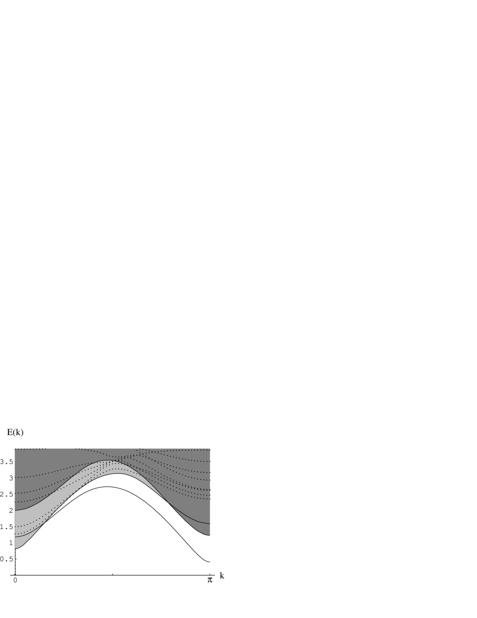
FIG. 3.: The spectrum for $\beta=0$ is shown. The lowest single particle triplet is shown as a solid line, with the lightly shaded region representing two-particle excitations and the dark region three particle excitations. Solid lines define the boundaries to the two and three particle continuum. Dotted lines indicate the spectrum of higher energy single-magnon excitations. The spin of these dotted excitations are, in order of increasing energy at $k=\pi$: 0,1,2,2,3,1,1,0.

FIG. 4.: The gap $\Delta_{\pi}$ to the lowest triplet excitation at momentum $k=\pi$ as a function of $\beta$ is shown.

$\beta$	$E_{0}$	exact	best numerical
$-\frac{1}{3}$	$-0.66666667$	$\frac{2}{3}$
$0$	$-1.40138$	-	$-1.401484038971(4)$
$0.6$	$-2.9184$	-
$1.0$	$-3.98455$	$-4$

TABLE I.: Ground state energy per site

REFERENCES

- [1] K. G. Wilson, Rev. Mod. Phys. 47, 773 (1975).
- [2] S.R. White, Phys. Rev. Lett. 69, 2863 (1992).
- [3] S.R. White, Phys. Rev. B 48, 10345 (1993).
- [4] S. Östlund and S. Rommer, Phys. Rev. Lett. 75, 3537 (1995).
- [5] S.R. White and D.A. Huse, Phys. Rev. B 48, 3844 (1993).
- [6] E.S. Sørensen and I. Affleck, Phys. Rev. Lett. 71, 1633 (1993).
- [7] E.S. Sörensen and I. Affleck, Phys. Rev. B 49, 15771 (1994).
- [8] S. Qin, T.K Ng and Z.B Su, preprint cond-mat/9502047.
- [9] I. Affleck, T. Kennedy, E.H. Lieb and H. Tasaki, Phys. Rev. Lett. 59, 799 (1987); Commun. Math. Phys. 115, 477 (1988).
- [10] T. Kennedy and H. Tasaki, Commun. Math. Phys. 147, 431 (1992); T. Kennedy, J. Phys.: Cond. Mat. 6, 8015 (1994). In the latter paper, a very general variational calculation is performed on the S=1 model, but roughly 200 variational parameters are required to get an accuracy comparable to what we accomplish with eight.
- [11] L. Accardi, Phys. Rep. 77, 169 (1981).
- [12] M. Fannes, B. Nachtergaele, R.F. Werner, Europhys. Lett. 10, 633 (1989); Commun. Math. Phys. 144, 443 (1992).
- [13] A. Klümper, A. Schadschneider and J. Zittarz, Europhys. Lett. 24 293 (1993), C. Lange, A. Klümper and J. Zittarz, cond-mat/9409107.
- [14] M. den Nijs and K. Rommelse, Phys. Rev. B 40, 4709 (1989).
- [15] L.A. Takhtajan, Phys. Lett. 87 A, 205 (1982); H.M. Babujian, Phys. Lett. 90 A, 479 (1983); Nucl. Phys. B 215, 317 (1983).
- [16] E.S. Sørensen and I. Affleck, Phys. Rev. B 49, 13235 (1994).
- [17] T. Sakai and M. Takahashi, Phys. Rev. B 42, 1090 (1990).
- [18] J. Oitmaa, J.B. Parkinson and J.C. Bonner, J. Phys. C 19, L595 (1986).
- [19] T. Xiang and G.A. Gehring, Phys. Rev. 48, 303 (1993).
- [20] R.J. Bursill, T. Xiang and G.A. Gehring, J. Phys. A 28, 2109 (1994).
- [21] U. Schollwöck, Th. Jolicœur and T. Garel, Phys. Rev. B 53, 3304 (1996).