Dynamic Behavior of Spin Glass Systems on Quenched $\phi^{3}$ Graphs

Abstract

We study the dynamical out-of-equilibrium behavior of a $J=\pm 1$ Ising spin glass on quenched $\phi^{3}$ graphs. We show that magnetization and energy decay with a power law behavior, with exponents that are linear in $\frac{T}{T_{c}}$. Quenched $\phi^{3}$ graphs turn out to be a very effective way to study numerically mean field spin glasses.

cond-mat/9606194

Spin models on quenched $\phi^{3}$ graphs have been considered in the last few years as a possible effective way to define mean field models [1, 2]. In general one can consider $\phi^{z}$ random quenched graphs (with the limit $z\to\infty$ coinciding with the usual Sherrington-Kirkpatrick definition of the mean field). One obtains mean field behavior on such graphs for the same reason as on the Bethe lattice because of the tree-like local structure, but the drawback of a dominant surface contribution is absent. It is not clear whether this approach is advantageous analytically since the large number law cannot be applied in a straightforward manner, and in general calculations appear more involved than for the SK approach. On the other hand from the numeric point of view there are distinct advantages, since in this case one is dealing with a model with local interaction where one spin update takes the order of $z$ operations and not order volume. A parenthetic warning is probably in order at this point - the fact that computation is faster does not necessarily imply that the model is the best choice. One has to perform the simulation to check. For example, the hypercube definition of the mean field (see for example Parisi-Ritort in [1]) undergoes very strong finite size effects, that can make the analysis of the thermodynamic limit very obscure.

Gardner, Derrida and Mottishaw [3] have drawn attention to the fact that when looking at the dynamical behavior of disordered systems one can expect to see power law behavior. The complex landscape does not allow a fast exponential convergence. Their calculation (that integrates exactly a small number of time steps) establishes that the $T=0$ parallel dynamics from a magnetized state leads to a non-zero magnetization expectation value with a power correction. Eisfeller and Opper in ref. [4] introduced a new approach combining the dynamical functional method and a Monte Carlo simulation of a stochastic single-spin equation that allowed the determination with good precision of the value of the remanent magnetization, $m(\infty)=0.474$ and of the exponent $\mu(T=0)=0.184$ where

$$m(t)-m(\infty)\simeq(t/\tau)^{-\mu}.$$ (1)

In a recent work Ferraro[5] has generalized the Eisfeller-Opper work to the non-zero temperature case. In this way he has been able to establish that in the SK model the magnetization and the energy do decay with power laws. Such a generalization of the Eisfeller-Opper method to non-zero $T$ does indeed allow a good determination of the magnetization exponent (which turns out to be linear in $T/T_{c}$), but is less effective for the energy exponent. Very large scale dynamical simulations of the SK model from Rossetti [6] allowed a first direct Monte Carlo determination of the power exponents, and showed that in the case of the SK definition of the mean field numerical simulation is very tough due to the non-local interaction. For comparison it is worth noting what happens in real experiments with typical spin glasses (see for example [7]). If one fits with the form in equation (1) one finds that $\mu(T)\simeq 0.4T/T_{c}$, where $\tau$ is of the order of magnitude of the microscopic time for single spin flip, and turns out not to depend on $T$.

Given the difficulty of simulations with non-local interactions and the success of the $\phi^{3}$ graph simulations in reproducing static mean-field spin glass behavior [2] it is obviously tempting to investigate dynamical aspects of spin glass behavior with $\phi^{3}$ graphs. We have thus carried out a Monte Carlo simulation of the dynamics of a spin glass model on $\phi^{3}$ graphs for different temperature values and graph sizes. The principal measurements of interest in such a simulation are the time series of the energy and the magnetization, which we have measured in the standard fashion. From these time series we have systematically analyzed the time dependence of magnetization and energy, starting from a cold system with $m=1$. We have tried to find the temporal regions where we could exhibit a clean scaling behavior, and we discuss our findings in the following.

We have used integer uniformly distributed quenched random couplings $J=\pm 1$ (i.e. the probability distribution for the quenched bond distribution is $P(J)=1/2\delta(J+1)+1/2\delta(J-1)$) in our simulations here because the earlier static simulations carried out with this distribution were known to give convincing agreement with theoretical calculations [2]. This provided a degree of confidence in the code used. One slight drawback of this choice is that with integer couplings the system has a energy gap, and at too low $T$ values the system will not be able to converge to equilibrium (as we have checked in preliminary numerical simulations). In order to avoid this problem we have kept our $T$ values sufficiently high to avoid the influence of the gap. In any case, preliminary work with a gaussian coupling distribution where there is no gap indicates no fundamental differences with the results here.

For each of the graph sizes simulated 100 different $\phi^{3}$ graphs were generated and a massively parallel processor (the Intel Paragon) was employed to allow the quenched averaging to be performed in situ. As we are interested in the “real” dynamics of the model we employed a simple single spin Metropolis update. The actual runs were of relatively short duration ($O(10^{4})$ sweeps) as this was sufficient to cover the temporal regions of interest. As we have indicated above, a cold start with $m=1$ was used.

Having dealt with the preliminaries, we now discuss the magnetization data in general terms. We start from a magnetized system, and observe the magnetization decay. On general grounds, we expect three different temporal regimes. At short times there is a transient, non-universal region, which is expected to depend on the details of the dynamics (in our case Metropolis). For intermediate times we expect to be able to detect a region with time power decay, where

$$m(t)\simeq\frac{A}{t^{\mu}}\ .$$ (2)

Finally, at large times on a finite graph we reach a plateau value for the remanent magnetization. The decay rate to this plateau (when, due to the finite extent of the sample, the system has reached the bottom of a valley) is a new dynamical effect, that can again be different from the previous phase. We will see that it is probably an exponential decay to the bottom of the hole. As we already have observed, in a finite size system of volume $V$ one expects

$$m(t)\to_{t\to\infty}m_{(V)}\ .$$ (3)

In fact our data is compatible with a zero infinite volume limit for $m_{(V)}$

$$m_{(V)}\to_{V\to\infty}0\ ,$$ (4)

though other possibilities are not excluded within the accuracy of the measurements.

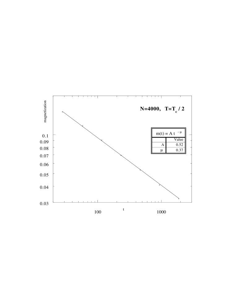
Figure 1: Magnetization versus Monte Carlo time in log-log scale. Here $N=4000$, $T=\frac{T_{c}}{2}$, $t$ ranging from $20$ to $2500$.

Let us now discuss in some detail the analysis of the magnetization data on the largest graphs ($N=4000$ vertices) simulated. For this graph size we have data samples of $20,000$ lattice sweeps at each $\beta$ value. The coldest data we will discuss is at $\beta=2\beta_{c}$ ($\beta_{c}\simeq.881$ for the $J=\pm 1$ distribution on $\phi^{3}$ graphs). For lower temperature values the discreteness of our couplings starts to play a role, and it is difficult to be sure of having determined the asymptotic power behavior. In fig. (1) we plot the data we use for our best fit. We use here times from $t_{min}=20$ to $t_{max}=2500$. Our best fit, drawn in the figure, gives an exponent $\mu=0.37$. This fit is very stable. Repeating it by doubling the confidence window both at small times and at large times (i.e. by selecting $t_{min}=40$ and $t_{max}=1250$) we find $\mu=0.37$.

The magnetization data at $\beta=2\beta_{c}$ converges to a plateau in our large time region (i.e. $t\simeq 15000$). A fit to a single power converging to a constant plateau does not work. In order to make the fit work one has to add higher power terms or an exponential decay (see later). The physics of what is happening is quite clear: we have a power decay for intermediate times, and at large times the finite volume system reaches the finite size value of the magnetization. The decay to such a finite value is not governed by the asymptotic power law we measure in the intermediate time region, and is probably (but not certainly) exponential.

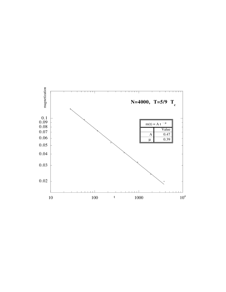
Figure 2: Magnetization versus Monte Carlo time in log-log scale. Here $N=4000$, $T=\frac{5T_{c}}{9}$, $t$ ranging from $20$ to $2500$.

In fig. (2) we plot the magnetization data at $\beta=\frac{9}{5}\beta_{c}$. Here the last point is already slightly off a good power fit because the time needed to reach the plateau is larger for lower $T$ values. We report this fit in order to give a feeling of the kind of systematic effects one gets, and because the fit with $t_{max}=1250$ gives for the first two significant digits of the exponent the same result. Again, the fit is stable. The fit in fig. (3), at $\beta=\frac{8}{5}\beta_{c}$, uses only time points ranging from $40$ to $1250$, but its quality, with an exponent of $\mu=.45$, is again very good.

Power fits for values of $T$ closer to $T_{c}$ are equally good, and we report their results in Table (1). The time window we use moves to short times when $T\to T_{c}$ as can be seen in fig. (4) for the time series at $T=T_{c}$. At $T_{c}$ the presence of a finite expectation value for $m$ due to the finite graph size is very clear. In fig. (5) we try an exponential fit to the decay to the finite size plateau which in this case is reached after only $100$ Monte Carlo sweeps. The exponential fit is very good. In summary, a power fits well in the intermediate time region, while an exponential fit explains very well the large time region. A fit with additional, different power terms is also able to fit the large time data: we consider our evidence for the existence of such an exponential behavior as only qualitative.

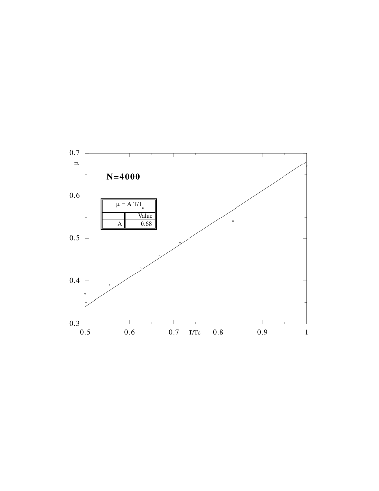
Figure 6: The magnetization time decay exponent $\mu$ versus $\frac{T}{T_{c}}$ for $N=4000$. The straight line passing through the origin is the best fit to the data.

Having established the power law decay at intermediate times, we now discuss the behavior of the exponent as the temperature is varied. In fig. (6) we show $\mu(\frac{T}{T_{c}})$. The straight line passing through the origin is our best fit to the data. The linear fit works well from $T_{c}$ down to $0.6$ $T_{c}$, while around $\frac{1}{2}$ $T_{c}$ the fit slightly undershoots the data point. Determining the exponent at low $T$ values becomes quite difficult (because it becomes small!) so such a small discrepancy is probably not a problem. Our conclusion is that

$$\mu(T)\simeq\frac{2}{3}\frac{T}{T_{c}}\ ,$$ (5)

in a large $T$ region in the broken phase. The best estimate from both Ferraro [5] and Rossetti [6]for the magnetization exponent is a linear dependence over $T/T_{c}$ with coefficient $1$, while, as we have already remarked, experiments favor a value close to $.4$. By a happy coincidence we find $2/3$, which lies between these two values. With the precision allowed by statistical and systematic errors (both in numerical simulations and, as far as we can understand, in real experiments) this is a very satisfactory result. Fits of magnetization time series on smaller graphs confirm the findings on the $N=4000$ graphs. For example with $N=3000$ we estimate $\mu(T_{c}/2)=.36$, and $\mu(5T_{c}/6)=.55$, in very good agreement with the results of table (1).

We close this section with two final remarks about the magnetization time series. Firstly, we emphasize again that the evidence for a final exponential approach to the plateau value is not overwhelmingly compelling, being mainly based on data close to $T_{c}$. Far from $T_{c}$ after $20,000$ sweeps we are still quite far from the plateau. In all cases fits done by allowing for two or three different powers also work quite well. Secondly the plateau value for the magnetization looks quite constant with $T$ in the broken phase. At $T_{c}$ for $N=4000$ we have $m_{\infty}\simeq 0.013$, at $N=3000$ we have $m_{\infty}\simeq 0.0145$. The remanent magnetization is becoming smaller with increasing volume, but we cannot be sure about the absence of a remanent magnetization at non-zero $T$. We stress that our measurements of power law do not rely on that, since we have selected a scaling region far away from the asymptotic (zero or non-zero) limit.

The discussion of the energy exponent $\epsilon$,

$$E(t)\simeq E_{\infty}-\frac{E_{1}}{t^{\epsilon}}$$ (6)

goes along very similar lines. Here we can fit up to larger times: it is only very close to $T_{c}$ that the power behavior is spoiled, even for times up to $t=20000$. The difference with the behavior of the magnetization, where all of the non-zero plateau at $t=\infty$ is probably due to finite size effects, is considerable. At $T=\frac{T_{c}}{2}$ fitting from $t=100$ to $t=20000$ we find a stable result, and a perfect fit with a very low $\chi^{2}$ value. We report the best fits to the exponents $\epsilon(T)$ in table (2).

For lower $\beta$ values we only have to discard a few more Monte Carlo points to get a good fit. Only right at $T=T_{c}$ does it seem that the asymptotic (non-simple power) behavior is encountered too early to get a good determination of the critical exponent. In this case larger graphs are probably needed.

In fig. (7) we plot our results for $\epsilon$ as a function of $\frac{T}{T_{c}}$, and our best linear fit (that is very good). The best fit gives

$$\epsilon\simeq 0.9\ \frac{T}{T_{c}}\ .$$ (7)

We note that this is the first time that it has been possible to get an estimate of the dependence of the energy exponent on $T$ for mean-field like systems. Results from the large scale simulation by Rossetti [6] for SK model are good but not as clear cut as the ones we are able to find here, while the infinite volume approach by Eisfeller and Opper [4] and Ferraro [5] gives clear results for the magnetization exponent but not for the energy exponent.

To summarize, we believe we have attained a double goal. Firstly, we have shown that models on $\phi^{3}$ graphs are good definitions of mean field spin glasses even where the dynamical behavior is concerned. Secondly, we have determined with good numerical precision the exponents of the power decay of magnetization and energy. This opens the way to a more systematic use of $\phi^{3}$ graphs for performing a numerical analysis of spin glasses.

ACKNOWLEDGEMENTS

We thank G. Parisi for interesting comments.

The bulk of the simulations were carried out on the Front Range Consortium’s 208-node Intel Paragon located at NOAA/FSL in Boulder. CFB is supported by DOE under contract DE-FG02-91ER40672 and by NSF Grand Challenge Applications Group Grant ASC-9217394. CFB and DAJ were partially supported by NATO grant CRG-951253. DAJ, CN and EM are also supported in part by EC HCM network grant CHRXCT930343.

$\frac{T}{T_{c}}$	time window	$\mu$
$1/2$	$20-2500$	$0.37$
$5/9$	$20-2500$	$0.39$
$5/8$	$20-1250$	$0.43$
$2/3$	$10-625$	$0.46$
$5/7$	$10-315$	$0.49$
$5/6$	$10-160$	$0.54$
$1$	$5-77$	$0.67$

Table 1: Magnetization time decay exponent $\mu$ for different $T$ values. $N=4000$. We also show the time window used for determining the exponent.

$\frac{T}{T_{c}}$	$\epsilon$
$1/2$	$0.45$
$5/9$	$0.50$
$5/8$	$0.53$
$2/3$	$0.58$
$5/7$	$0.64$
$5/6$	$0.75$
$1$	$0.92$

Table 2: Energy time decay exponent $\epsilon$ for different $T$ values. $N=4000$.

Figure 3: Magnetization versus Monte Carlo time in log-log scale. Here $N=4000$, $T=\frac{5T_{c}}{8}$, $t$ ranging from $40$ to $1250$.

Figure 4: Magnetization versus Monte Carlo time in log-log scale. Here $N=4000$, $T=T_{c}$, $t$ ranging from $4$ to $77$.

Figure 5: Magnetization versus Monte Carlo time in log-log scale. Here $N=4000$, $T=T_{c}$, $t$ ranging from $9$ to $20000$.

Figure 7: The energy time decay exponent $\epsilon$ versus $\frac{T}{T_{c}}$ for $N=4000$. The straight line passing through the origin is the best fit to the data.

References

- [1] J. R. Banavar, D. Sherrington and N. Sourlas, J. Phys. A20 (1987) L1; M. Mezard and G. Parisi, Europhys. Lett. 3 (1987) 1067; Y. Y. Goldschmidt and C. de Dominicis, Phys. Rev. B41 (1990) 2184; G. Parisi and F. Ritort, J. Phys. I France 3 (1993) 969; C. Bachas, C. de Calan and P. Petropoulos, J. Phys. A27 (1994) 6121.
- [2] C. Baillie, D. A. Johnston and J. P. Kownacki, Nucl. Phys. B432 (1994) 551; C. Baillie, W. Janke, D. A. Johnston and P. Plechac, Nucl. Phys. B450 (1995) 730.
- [3] E. Gardner, B. Derrida and P. Mottishaw, J. Phys. (france) 48 (1987) 741.
- [4] H. Eisfeller and M. Opper, Phys. Rev. Lett. 68 (1992) 2094;
- [5] G. Ferraro, cond-mat/9407091.
- [6] D. Rossetti, Comportamento Dinamico del Modello di Campo Medio dei Vetri di Spin, Tesi di Laurea Università di Roma La Sapienza (1995), unpublished.
- [7] J. Souletie, Ann. Phys. Fr. 10 (1985) 69.