Almost-Hermitian Random Matrices:
Eigenvalue Density in the Complex Plane

Abstract

We consider an ensemble of large non-Hermitian random matrices of the form $\hat{H}+i\hat{A}_{s}$, where $\hat{H}$ and $\hat{A}_{s}$ are Hermitian statistically independent random $N\times N$ matrices. We demonstrate the existence of a new nontrivial regime of weak non-Hermiticity characterized by the condition that the average of $N\mbox{Tr}\hat{A}_{s}^{2}$ is of the same order as that of $\mbox{Tr}\hat{H}^{2}$ when $N\to\infty$. We find explicitly the density of complex eigenvalues for this regime in the limit of infinite matrix dimension. The density determines the eigenvalue distribution in the crossover regime between random Hermitian matrices whose real eigenvalues are distributed according to the Wigner semi-circle law and random complex matrices whose eigenvalues are distributed in the complex plane according to the so-called “elliptic law”.

Recently there was a growth of interest in statistics of complex eigenvalues of large random matrices, both in physical and mathematical literature (see Refs. 1 - 20).

Non-Hermitian random Hamiltonians appear naturally when one deals with quantum scattering problems in open chaotic systems[7, 8, 11, 15, 16, 18], studies a motion of flux lines in superconductors with columnar defects [19] or is interested in chiral symmetry breaking in quantum chromodynamics [20]. Complex random matrices appear also in studies of dissipative quantum maps [6, 9]. On the other hand, closely related ensembles of real asymmetric random matrices enjoy applications in neural network dynamics [5, 12] and in the problem of the localization transition of random heteropolymer chains [21].

The actual progress in understanding the properties of random matrices with complex eigenvalues is rather limited, however. Most of the known results refer to the case of strong non-Hermiticity or asymmetry. Namely, they deal with those types of matrices for which the real and imaginary parts of complex eigenvalues $Z_{j}=X_{j}+iY_{j}$ are typically of the same order when the matrix dimension tends to infinity.

As the most well-known example, we mention an ensemble of complex $N\times N$ matrices $\hat{J}$ with the density of joint probability distribution of matrix entries of the form

$${\cal P}(\hat{J})=C_{N}^{-1}\exp\Big{[}-\frac{N}{J_{0}^{2}(1-\tau^{2})}\ \mbox{Tr}(\hat{J}\hat{J}^{\dagger}-\tau\ \mbox{Re}\ \hat{J}^{2})\Big{]},$$ (1)

where $\tau$ is real, $-1\leq\tau\leq 1$, and $C_{N}=[\pi^{2}J_{0}^{4}(1-\tau^{2})/N^{2}]^{N^{2}/2}$. In the large-$N$ limit the eigenvalues of $\hat{J}$ are uniformly distributed in the ellipse $X^{2}/(1+\tau)^{2}+Y^{2}/(1-\tau)^{2}\leq J_{0}^{2}$ [3, 4, 10].

Denote by $J_{kl}$ a matrix element of $\hat{J}$. Eq. (1) implies that: (i) complex variables $J_{kl}$ are Gaussian with mean zero and variance $\langle|J_{kl}|^{2}\rangle=J_{0}^{2}/N$, (ii) the real and imaginary parts of $\hat{J}$ are statistically independent, and (iii) among all the random variables $J_{kl}$, $1\leq k,l\leq N$, only $J_{kl}$ and $J_{lk}$ are pairwise correlated with the magnitude of correlations determined by the covariance $\langle J_{kl}J^{*}_{lk}\rangle=\tau J_{0}^{2}/N$. The ensemble defined by Eq. (1) interpolates between the well-known Gaussian ensemble of Hermitian matrices (GUE) [22] and Ginibre’s ensemble of complex matrices [1]. The degree of non-Hermiticity is controlled by the absolute value of $\tau$. If $\tau=1$ or $\tau=-1$ we have an ensemble of Hermitian or skew-Hermitian matrices and the above mentioned ellipse degenerates into an interval of real or purely imaginary eigenvalues. On the other hand, if $\tau=0$ then all $J_{kl}$ are mutually independent and we have a maximum of asymmetry. In that case the eigenvalues are uniformly distributed in the unit circle [1, 22, 2].

The above mentioned ensemble of non-Hermitian random matrices can be represented in another form. Each matrix $\hat{J}$ can be decomposed into a sum of its Hermitian and skew-Hermitian parts: $\hat{J}=\hat{H}+i\hat{A}_{s},$ where $\hat{H}=(\hat{J}+\hat{J}^{\dagger})/2$ and $\hat{A}_{s}=(\hat{J}-\hat{J}^{\dagger})/2i$. By Eq. (1), the Hermitian matrices $\hat{H}$ and $\hat{A}_{s}$ are statistically independent and follow the Gaussian distributions ${\cal P}(\hat{H})\propto\exp\{-2N/[(1+\tau)J_{0}^{2}]\ \mbox{Tr}\hat{H}^{2}\}$ and ${\cal P}(\hat{A}_{s})\propto\exp\{-2N/[(1-\tau)J_{0}^{2}]\ \mbox{Tr}\hat{A}_{s}^{2}\}$, respectively. In this representation interpolation mentioned above becomes even clearer. For instance, when $\tau$ approaches 1 variations of $\hat{A}$ around its mean value vanish and $\hat{J}=\hat{H}$ in the limit of $\tau=1$.

For our purpose it is convenient to introduce new variables, $J^{2}=J_{0}^{2}(1+\tau)/4$ and $v^{2}=(1-\tau)/(1+\tau)$, and rewrite the ensemble defined by Eq. (1) as

$$\hat{J}=\hat{H}+iv\hat{A},$$ (2)

where now each $\hat{H}$ and $\hat{A}$ is taken from identical and independent Gaussian ensembles of Hermitian matrices defined by the probability densities:

$${\cal P}(\hat{H})\propto\exp{\Big{(}-\frac{N}{2J^{2}}\mbox{Tr}\hat{H}^{2}\Big{)}}\;\;\mbox{and}\;\;{\cal P}(\hat{A})\propto\exp{\Big{(}-\frac{N}{2J^{2}}\mbox{Tr}\hat{A}^{2}\Big{)}}.$$ (3)

It is natural to use the parameter $v^{2}$ as a measure of non-Hermiticity (asymmetry) in our ensemble. As we mentioned, in the case of strong non-Hermiticity, i. e. when $v^{2}=O(1)$ as $N\to\infty$, the eigenvalues of $\hat{J}$ are uniformly distributed in an ellipse.

In the present paper we demonstrate the existence of a new non-trivial regime of weak non-Hermiticity determined by the condition $v^{2}N=O(1)$ as $N\to\infty$. In other words, we scale the parameter $v$ with the matrix dimension $N$ as $v=\alpha/\sqrt{N}$, $\alpha\geq 0$. In that regime of weak non-Hermiticity the “elliptic law” is not valid any longer and should be replaced by another distribution. The main goal of our publication is to derive the explicit form of this distribution.

In order to get better understanding of the chosen scaling it is instructive to consider first the limiting case of extremely weak non-Hermiticity. In this case one expects that the influence of adding the non-Hermitian matrices $iv\hat{A}$ to the Hermitian matrices $\hat{H}$ in Eq. (2) can be treated by regular perturbation theory.

When $v=0$ the eigenvalues $Z_{j}\equiv X_{j}$ of $\hat{J}\equiv\hat{H}$ are real and in the large-$N$ limit they are distributed according to the Wigner semi-circle law with the density $\rho_{sc}(X)=(2\pi J)^{-1}\sqrt{4-(X/J)^{2}}$. The mean separation $\Delta$ between adjacent eigenvalues can be estimated as $\Delta\propto J/N$. When a small non-Hermitian part $iv\hat{A}$ is taken into account, the eigenvalues $Z_{j}$ of $\hat{J}$ move into the complex plane and their shift can be estimated by first order perturbation theory. Namely, $\mbox{Re}\ Z_{j}=X_{j}$ and $\mbox{Im}\ Z_{j}=v\langle\phi_{j}\!\mid\hat{A}\mid\!\phi_{j}\rangle$, where $X_{j}$ and $\mid\!\phi_{j}\rangle$ are the ordered eigenvalues of $\hat{H}$ and their normalized eigenvectors, respectively. Let us estimate the magnitude of this shift. Introducing the notation $\hat{P}_{j}$ for the projection on $\mid\!\phi_{j}\rangle$, one can write $\mbox{Im}\ Z_{j}=v\mbox{Tr}\hat{A}\hat{P}_{j}$, so the variance of $Y_{j}\equiv\mbox{Im}Z_{j}$ is

$$\langle\ Y^{2}_{j}\ \rangle={\langle{\langle\ Y^{2}_{j}\ \rangle}_{\!A}\rangle}_{\!H}=v^{2}{\langle{\langle\ \big{|}\mbox{Tr}\hat{A}\hat{P}_{j}\big{|}^{2}\ \rangle}_{\!A}\rangle}_{\!H},$$ (4)

where the angle brackets ${\langle\cdot\rangle}_{H(A)}$ denote the averaging over the random matrices $\hat{H}(\hat{A})$ according to Eq. (3). Since $\hat{H}$ is statistically independent of $\hat{A}$, so is $\hat{P}_{j}$. As a result, one can perform the averaging over $\hat{A}$ in Eq. (4) explicitly:

$${\langle{\langle\ Y^{2}_{j}\ \rangle}_{\!A}\rangle}_{\!H}=\frac{4J^{2}}{N}{\langle\ \mbox{Tr}\hat{P}_{j}^{2}\ \rangle}_{\!H}.$$ (5)

Now noticing that $\hat{P}_{j}^{2}=\hat{P}_{j}$ and $\mbox{Tr}\hat{P}_{j}=1$ (as it must be for any projection), we obtain the deviation of $Y_{j}$, ${\langle\ Y^{2}_{j}\ \rangle}^{1/2}=2vJ/N$. Since we are using perturbation theory, this deviation has to be compared with the mean separation $\Delta$ of the unperturbed eigenvalues: ${\langle\ Y^{2}_{j}\ \rangle}^{1/2}\!/\Delta\propto v\sqrt{N}=\alpha$; so the case $\alpha\ll 1$ corresponds to well-defined perturbation theory.

The density $\rho(X,Y)$ of complex eigenvalues $Z_{j}$ can be calculated easily in the perturbative regime $\alpha\ll 1$. Indeed, $\rho(X,Y)=\langle\langle\ N^{-1}\sum_{j=1}^{N}\delta(X-X_{j})\delta(Y-Y_{j})\ \rangle_{\!A}\rangle_{\!H}$. Now employing the Fourier representation for $\delta(Y)$, one finds that

$$\rho(X,Y) = \frac{1}{2\pi N}\sum_{j=1}^{N}\int_{-\infty}^{\infty}dke^{ikY}\Big{\langle}\Big{\langle}\ \delta(X-X_{j})\exp{\Big{[}\frac{-i\alpha k}{\sqrt{N}}\mbox{Tr}\hat{A}\hat{P}_{j}\Big{]}}\ \Big{\rangle}_{\!\!A}\Big{\rangle}_{\!\!H}$$

$$= \frac{1}{2\pi N}\sum_{j=1}^{N}\int_{-\infty}^{\infty}dke^{ikY}\Big{\langle}\ \delta(X-X_{j})\exp{\Big{[}-\frac{(\alpha kJ/N)^{2}}{2}\mbox{Tr}\hat{P}^{\dagger}_{j}\hat{P}_{j}\Big{]}}\ \Big{\rangle}_{\!\!H}$$

$$= \frac{1}{N}\sum_{j=1}^{N}\big{\langle}\ \delta(X-X_{j})\ \big{\rangle}_{\!H}\frac{1}{2\pi}\int_{-\infty}^{\infty}dke^{ikY}\exp{\Big{[}-\frac{1}{2}\Big{(}\frac{\alpha kJ}{N}\Big{)}^{2}\Big{]}}$$

$$= \rho_{sc}(X)\rho(Y),$$

where

$$\rho(Y)=\frac{1}{\sqrt{2\pi}\tilde{a}}\exp\left(-\frac{Y^{2}}{2\tilde{a}^{2}}\right)$$ (6)

and $\tilde{a}=\alpha J/N$. We see that for $\alpha\ll 1$ the density of eigenvalues in the complex plane $X+iY$ is a simple product of the Wigner semicircular density $\rho_{sc}(X)=(2\pi J)^{-1}\sqrt{4-(X/J)^{2}}$ and the Gaussian $\rho(Y)$ from Eq. (6). On the other hand, it is natural to expect that when $\alpha\gg 1$ $\rho(X,Y)$ goes back to the mentioned uniform distribution inside an ellipse.

In order to get access to the distribution of eigenvalues in the complex plane $E=X+iY$ in the case of $\alpha=O(1)$ we use the fact that the two-dimensional density of these eigenvalues $\rho(X,Y)$ can be found if one knows the “potential” [4]:

$$\Phi(X,Y,\kappa)=\frac{1}{2\pi N}\left\langle\left\langle\ln{Det[(E-\hat{J})(E-\hat{J})^{\dagger}+\kappa^{2}\hat{I}]}\right\rangle_{\!\!A}\right\rangle_{\!H}$$ (7)

in view of the relation: $\rho(X,Y)=\lim_{\kappa\to 0}\partial^{2}\,\Phi(X,Y,\kappa)$, where $\partial^{2}$ stands for the two-dimensional Laplacian $\partial_{X}^{2}+\partial_{Y}^{2}$. To determine the potential for the present case of almost-Hermitian Gaussian random matrices we follow the method suggested earlier by two of us [18] and restore the potential from its derivative:

$$\frac{\partial^{2}\Phi}{\partial\kappa^{2}} = \frac{1}{2\pi N}\frac{d}{d\kappa}\lim_{\kappa_{b}\to\kappa}\frac{\partial}{\partial\kappa}\left\langle\left\langle\ln{Z(\kappa_{b},\kappa)}\right\rangle_{\!\!A}\right\rangle_{\!\!H}$$ (8)

$$Z(\kappa_{b},\kappa) = \frac{Det[(E-\hat{J})(E-\hat{J})^{\dagger}+\kappa^{2}\hat{I}]}{Det[(E-\hat{J})(E-\hat{J})^{\dagger}+\kappa_{b}^{2}\hat{I}]}.$$ (9)

It is convenient for our purpose to write down the determinants in the denominator and numerator of the generating function as:

$$Det[(E-\hat{J})(E-\hat{J})^{\dagger}+\kappa_{b}^{2}\hat{I}]=Det\left[\hat{M_{b}}\left(\begin{array}[]{cc}\kappa_{b}\hat{I}&i(E-\hat{J})\\ i(E-\hat{J})^{\dagger}&\kappa_{b}\hat{I}\end{array}\right)\hat{M}_{b}^{-1}\right]$$ (10)

$$Det[(E-\hat{J})(E-\hat{J})^{\dagger}+\kappa^{2}\hat{I}]=Det\left[\hat{M}\left(\begin{array}[]{cc}i(E-\hat{J})^{\dagger}&\kappa\hat{I}\\ \kappa\hat{I}&i(E-\hat{J})\end{array}\right)\hat{M}^{-1}\right]$$ (11)

where we used two matrices: $\hat{M}_{b}=\frac{1}{\sqrt{2}}\left(\begin{array}[]{cc}\hat{I}&-i\hat{I}\\ \hat{I}&i\hat{I}\end{array}\right);\quad\hat{M}_{b}^{\dagger}=\hat{M}_{b}^{-1}$ and $\hat{M}=\frac{1}{\sqrt{2}}\left(\begin{array}[]{cc}\hat{I}&-\hat{I}\\ \hat{I}&\hat{I}\end{array}\right);\quad\hat{M}^{\dagger}=\hat{M}^{-1}$.

Then one can find the following convergent representation for the generating function $Z(\kappa_{b},\kappa)$ in terms of a Gaussian integral over both commuting and anticommuting (Grassmannian) variables:

$$(-1)^{N}Z(\kappa_{b},\kappa) = \int[d\Psi]\exp\{-{\cal L}_{0}(\Psi)-{\cal L}_{1}(\Psi)\}$$ (12)

$${\cal L}_{0}(\Psi) = \kappa_{b}(\Psi^{\dagger}\hat{\Lambda}\hat{L}\Psi)+iX(\Psi^{\dagger}\hat{L}\Psi)-Y(\Psi^{\dagger}\hat{\sigma}_{0}\Psi)+(\kappa-\kappa_{b})(\Psi^{\dagger}\hat{K}\Psi)$$ (13)

$${\cal L}_{1}(\Psi) = -i\Psi^{\dagger}(H\otimes\hat{L})\Psi-\frac{\alpha}{N^{1/2}}\Psi^{\dagger}(\hat{A}\otimes\hat{\sigma}_{0})\Psi,$$ (14)

where $\Psi^{\dagger}=(\vec{S}^{\dagger}_{1},\vec{S}^{\dagger}_{2},\chi^{\dagger}_{1},\chi^{\dagger}_{2});\quad[d\Psi]=\prod_{p=1,2}{d\vec{S}_{p}d\vec{S}^{\dagger}_{p}d\chi_{p}d\chi^{\dagger}_{p}}$, with $\vec{S}_{p}$ and $\chi_{p}$ being $N-$component vectors of complex commuting and Grassmannian variables, respectively. The $4\times 4$ matrices $\hat{\Lambda},\hat{L},\hat{\sigma}_{0}$ and $\hat{K}$ are (block)diagonal of the following structure:

$$\begin{array}[]{r r r r r r}\hat{\Lambda}&=&\mbox{diag}(1,-1,1,-1);&\hat{L}&=&\mbox{diag}(1,-1,1,1);\\ \hat{K}&=&\mbox{diag}(0,0,1,-1);&\hat{\sigma_{0}}&=&\mbox{diag}(i\Sigma_{x},\Sigma_{x});\end{array}$$

and $\Sigma_{x}=\left(\begin{array}[]{cc}0&1\\ 1&0\end{array}\right)$.

Due to the normalization condition $Z(\kappa,\kappa)=1$ it is enough for our purpose to calculate the average $\left\langle\left\langle Z(\kappa,\kappa_{b})\right\rangle_{\!\!A}\right\rangle_{\!H}$. This can be done easily for the Gaussian distributions Eq. (3) and leads to the terms quartic in the components of the supervector $\Psi$ in the exponent of the integrand, Eq. (13). Further evaluation goes along lines suggested by Efetov in the theory of disordered systems [23]. A detailed introduction to the method as applied to random Hermitian matrices can be found in the review[24]. Here we outline only the general strategy: 1) To decouple quartic terms in the exponent of the integrand of the generating function by introducing a set of auxiliary integrations (the so-called Hubbard-Stratonovich transformation, see [24]); 2) To integrate out the $\Psi$-variables explicitly; and 3) Exploiting the limit $N\to\infty$ to integrate out some ("massive") degrees of freedom in the saddle-point approximation. After this is done the integral over the remaining ("massless") degrees of freedom can be represented in a form of the so-called zero-dimensional graded nonlinear $\sigma-$model introduced into physics by Efetov[23].

After this set of standard manipulations one arrives at the following expression for the density $\rho_{X}(y)$ of the scaled imaginary parts $y_{j}=2\pi{\rho_{sc}(X)}Y_{j}N$ of those eigenvalues $Z_{j}=X_{j}+iY_{j}$ whose real parts $X_{j}$ fall within a narrow window around the point $X$ of the spectrum:

$$\rho_{X}(y)=\frac{1}{2}\frac{\partial^{2}}{\partial y^{2}}\int_{0}^{\infty}duu\phi(y,u),$$ (15)

where

$$\phi(y,u)=i\displaystyle{\frac{\partial}{\partial u}}\int d\mu(Q)\mbox{Str}(\hat{K}\hat{Q})\,\times\exp\Big{[}-\frac{iu}{2}\mbox{Str}(\hat{Q}\hat{\Lambda})-\frac{iy}{2}\mbox{Str}(\hat{Q}\hat{\sigma})-\frac{a^{2}}{16}\mbox{Str}(\hat{Q}\hat{\sigma}\hat{Q}\hat{\sigma})\Big{]},$$ (16)

where $a=2\pi{\rho_{sc}(X)}\alpha$, $\hat{\sigma}=\mbox{diag}(\Sigma_{x},\Sigma_{x})$ and the (graded) matrices $\hat{Q}$ satisfying $\hat{Q}^{2}=-1$ are taken from the graded coset space $U(1,1/2)/U(1/1)\otimes U(1/,1)$, whose explicit parameterization can be found in [23, 24]. We also use the notation Str for the graded trace.

Still, the evaluation of the integral over the graded coset space in Eq. (16) and subsequent restoration of the density $\rho_{X}(y)$ is quite an elaborate task. We skip intermediate steps and present the final expression for $\phi(y,u)$ which one obtains after integrating out the Grassmannian variables:

$$\phi(y,u) = \langle I(z_{1},z_{2})\rangle_{Z}\equiv\frac{1}{2\pi}\int_{-\infty}^{\infty}\int_{-\infty}^{\infty}dz_{1}dz_{2}\exp{\left[-\frac{1}{2}(z_{1}^{2}+z_{2}^{2})\right]}I(z_{1},z_{2})$$ (17)

$$I(z_{1},z_{2}) = y\left[F_{2}\partial_{y}F_{1}-F_{1}\partial_{y}F_{2}\right]-\frac{a^{2}}{2}\left[F_{1}F_{2}+\partial_{y}F_{1}\partial_{y}F_{2}+\partial_{u}F_{1}\partial_{u}F_{2}-F_{2}\partial^{2}_{y}F_{1}-F_{1}\partial^{2}_{y}F_{2}\right]$$ (18)

where

$$F_{1}(y,u,z_{1},z_{2})=\frac{e^{-\sqrt{u^{2}+y_{b}^{2}}}}{\sqrt{u^{2}+y_{b}^{2}}};\quad F_{2}(y,u,z_{1},z_{2})=\frac{\sinh\sqrt{u^{2}+y_{f}^{2}}}{\sqrt{u^{2}+y_{f}^{2}}};$$ (19)

and $y_{b}=y-az_{1}/\sqrt{2};\,\,y_{f}=y-iaz_{2}/\sqrt{2}$.

It is easy to check that both functions $F_{1}$ and $F_{2}$ satisfy the relation:

$$\partial^{2}_{y}F_{1,2}=F_{1,2}-\frac{1}{u}\partial_{u}\left(u\partial_{u}F_{1,2}\right).$$ (20)

Now substitute Eq. (17) into Eq. (15) and notice (by multiple exploitation of Eq. (20) ) that $I(z_{1},z_{2})$ can be written as a full derivative over $u$. As a result, one obtains:

$$\rho_{X}(y) = \Big{\langle}[2+y\partial_{y}]\left[u(F_{1}\partial_{u}F_{2}-F_{2}\partial_{u}F_{1})\right]\left|{}_{u\to 0}\right.\Big{\rangle}_{\!Z}-$$ (22)

$$\Big{\langle}\frac{a^{2}}{2}\partial^{2}_{y}[F_{1}\partial_{u}(u\partial_{u}F_{2})]\left|{}_{u\to 0}\right.-\frac{a^{2}}{2}\partial_{y}[u(F_{2}\partial^{2}_{uy}F_{1}-\partial_{y}F_{1}\partial_{u}F_{2})]\left|{}_{u\to 0}\right.\Big{\rangle}_{\!Z},$$

where $\langle...\rangle_{Z}$ denotes the integration over $z_{1},z_{2}$ with the Gaussian weight, see Eq. (17). When performing the limiting procedure $u\to 0$ in Eq. (22). one notices that all terms are proportional to a $\delta$-function: $\delta(y_{b})$, or its derivatives. This fact allows one to perform the integration over $z_{1}$ explicitly, and after some simple algebraic manipulations one arrives at the following expression:

$$\rho_{X}(y)=\frac{1}{\sqrt{2\pi}a}\exp\left(-\frac{y^{2}}{2a^{2}}\right)\int_{0}^{1}dt\cosh(ty)\exp{(-a^{2}t^{2}/2)},$$ (23)

where $a=2\pi\rho_{sc}(X)\alpha$ and $y=2\pi\rho_{sc}(X)YN$, $X$ and $Y$ being the real and imaginary parts of the complex eigenvalues in the ensemble of random matrices $\hat{J}$ given by Eqs. (2)-(3).

The distribution Eq. (23) constitutes the main result of the present publication. It correctly reproduces all the anticipated limiting cases. When $a\gg 1$ one can effectively put the upper boundary of integration in Eq. (23) to be infinity due to the Gaussian cut-off of the integrand at $t\sim 1/a\ll 1$. This immediately results in the uniform density $\rho_{X}(y)=(2a^{2})^{-1}$ inside the interval $|y|\leq a^{2}$ and vanishing density outside this interval. Recalling the definition of the variable $y$ and the parameter $a$, we are back to the familiar “elliptic law”. In the opposite limiting case $a\ll 1$ one obtains:

$$\rho_{X}(y)=\frac{1}{(2\pi)^{1/2}a}\exp\Big{(}-\frac{y^{2}}{2a^{2}}\Big{)}\frac{\sinh{y}}{y}$$

which matches the perturbative result Eq. (6) as long as $y\ll 1$. The fact that remote tails $y\gtrsim 1$ are not captured correctly by perturbative treatment can be understood easily: the condition $y\sim 1$ means that the imaginary parts $Y_{j}$ of the complex eigenvalues is of the same order as the mean spacing $\Delta=(\rho_{sc}(X)N)^{-1}$ between the real eigenvalues of the unperturbed Hermitian matrix $\hat{H}$. First order perturbation theory is obviously insufficient to obtain those complex eigenvalues correctly.

It is worth mentioning that we have restricted ourselves to Gaussian distributions of random matrices $\hat{H}$ and $\hat{A}$ mainly for the sake of simplicity of presentation of the supersymmetry calculations. More general distributions of matrices $\hat{H}$ and $\hat{A}$ can be considered and supersymmetry calculations can be performed along the line of [25, 26]. For instance one can consider random matrices $\hat{H}$ and $\hat{A}$ whose entries are independent Bernoulli variables taking $\pm b$ with equal probability or are uniformly distributed in an interval. Actually, we have arguments that the universality of the eigenvalue distribution in the crossover regime is extremely high and is not restricted to the case when the corresponding Hermitian matrices $\hat{H}$ have the semi-circle eigenvalue density. For example, one can consider non-Gaussian distributions of matrices $\hat{H}$ and $\hat{A}$ with the density of the form ${\cal P}(\hat{H})\propto\exp\{-N\mbox{Tr}V(\hat{H})\}$ (the so-called invariant ensembles, see [27, 28, 29, 30, 31, 32, 33]). Then the formula Eq. (23) is still valid, provided the semi-circular density $\rho_{sc}$ in the definitions of $y$ and $a$ is replaced by the actual mean level density at given point of the spectrum .

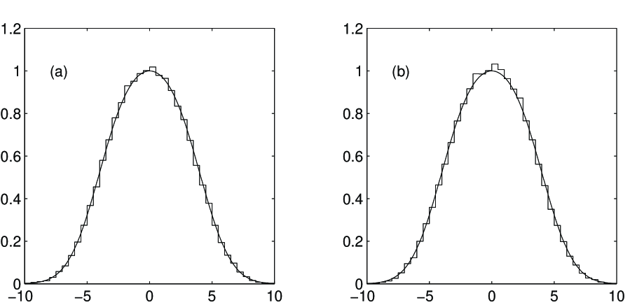
FIG. 1.: Histograms of distributions of the scaled imaginary parts of complex eigenvalues for a) Gaussian and b) Bernoulli distribution of matrix elements, see the text.

The distribution Eq. (23) has been derived in the limit of infinite matrix dimension. However, numerical computations show that Eq. (23) well approximates the distribution of complex eigenvalues for ensembles of random matrices (3) of a moderate dimension. In Fig. 1 we present results of numerical diagonalization of random matrices of dimension $N=30$. For each plot we generated a set of 20000 random matrices $\hat{J}=\hat{H}+i\frac{1}{\sqrt{N}}\hat{A}$ sampling a Gaussian distribution (random matrices follow distributions of Eq. (6) with $2J^{2}=1$) for plot (a) and a Bernoulli distribution (functionally independent matrix elements of $\hat{H}$ and $\hat{A}$ are statistically independent random variables taking $\pm 1/\sqrt{2N}$ with equal probability) for plot (b). Then matrices were diagonalized and their eigenvalues $Z_{j}$ falling into a small energy window, $|\mbox{Re}\ Z_{j}|\leq 0.2$, were selected. The imaginary parts of the selected eigenvalues were counted and the corresponding histograms along with the infinite-$N$ theoretical density $\rho_{X=0}(y)$ (solid curves) were plotted against the scaled variable $y_{j}=2\pi{\rho_{sc}(0)}Y_{j}N$. In both plots, the ordinate is scaled in units of $\max_{y}\rho_{X=0}(y)$.

It is worth mentioning that our derivation based on the supersymmetry formalism [23, 24] being in general quite satisfactory should be considered as a heuristic one from the point of view of rigorous mathematics. In a more detailed publication [34] we shall give a rigorous mathematical derivation of our main result, Eq. (23) for the case of Gaussian Matrices $\hat{H},\hat{A}$ and also show the mentioned universality of the found distribution for several classes of more general random matrices.

At the moment we failed to derive the analogous expression for almost-symmetric (slightly asymmetric) real random matrices due to unsurmountable technical problems. At the same time there are reasons to suspect that for the latter case the distribution might be different in its form from Eq. (23). It would be of much interest to try to attack this problem by different methods, e.g. starting from the known joint probability density for eigenvalues of asymmetric random matrices[10, 13].

In conclusion, we derived the explicit expression describing the density of complex eigenvalues of almost-Hermitian random matrices. It describes the crossover regime from the Wigner semi-circle law typical for random Hermitian matrices to the “elliptic law” typical for strongly non-Hermitian matrices.

The authors acknowledge financial support of Deutsche Forschungsgemeinschaft under Grant No SFB237. Numerical computations were performed at Institut für Mathematik, Ruhr-Universität-Bochum with the help of the MATLAB software package.

REFERENCES

• [1] Ginibre J 1965 J. Math. Phys. 6 440
• [2] Girko V L 1985 Theor. Prob. Appl. 29 694
• [3] Girko V L 1986 Theor. Prob. Appl. 30 677
• [4] Sommers H-J, Crisanti A, Sompolinsky H and Stein Y 1988 Phys. Rev. Lett. 60 1895
• [5] Sompolinsky H, Crisanti A and Sommers H-J 1988 Phys. Rev. Lett. 61 259
• [6] Grobe R, Haake F and Sommers H-J 1988 Phys. Rev. Lett. 61 1989
• [7] Sokolov V V and Zelevinsky V G 1988 Phys. Lett. B 202 10
• [8] Sokolov V V and Zelevinsky V G 1989 Nucl.Phys. A 504 562
• [9] Haake F 1991 Quantum Signature of Chaos (Berlin, Heidelberg, New York: Springer)
• [10] Lehmann N and Sommers H-J 1991 Phys. Rev. Lett. 67 941
• [11] Haake F, Izrailev F, Lehmann N, Saher D and Sommers H-J 1992 Z. Phys. B 88 359
• [12] Doyon B, Cessac B, Quoy M and Samuelidis M 1993 Int. J. Bifurc. Chaos 3 279
• [13] Edelman A 1993 The Circular Law and the Probability that a Random Matrix Has $k$ Real Eigenvalues; Preprint, available at http://theory.lcs.mit.edu/comprehensive.html
• [14] Edelman A, Kostlan E and Shub M 1994 J Amer. Math. Soc. 7 247
• [15] Lehmann N, Saher D, Sokolov V V and Sommers H-J 1995 Nucl. Phys. A 582 223
• [16] Müller M, Dittes M-M, Iskra W and Rotter I 1995 Phys. Rev. E 52 5961
• [17] Khoruzhenko B 1996 J. Phys. A: Math. Gen 29 L165
• [18] Fyodorov Y V and Sommers H-J 1995 “Statistics of S-matrix poles in few-channel chaotic scattering: crossover from isolated to overlapping resonance”, To appear in JETP Letters (June, 1996); Preprint cond-mat/9507117 available at cond-mat@xxx.lanl.gov
• [19] Hatano N and Nelson D R 1996 “Localisation transition in non-Hermitian quantum mechanics”, Preprint cond-mat/9603165 available at cond-mat@xxx.lanl.gov
• [20] Stephanov M A 1996 Phys. Rev. Lett. 76 4472
• [21] Nechaev S, private communication
• [22] Mehta M-L 1967 Random Matrices and the Statistical Theory of Energy Levels (Academic: New York)
• [23] Efetov K B 1983 Adv. Phys. 32 53
• [24] Fyodorov Y V 1995 in “Mesosocopic Quantum Physics”, Les Houches Summer School, Session LXI,1994, edited E.Akkermans et al., Elsever Science, p.493
• [25] Mirlin A D and Fyodorov Y V 1991 J. Phys. A:  Math. Gen 24 227
• [26] Fyodorov Y V 1995 and Sommers H-J Z.Phys.B 99 123
• [27] Brezin E, Itzykson C, Parisi G and Zuber J-B 1978 Comm. Math. Phys 59 35
• [28] Bessis D, Itzykson C and Zuber J 1980 Adv. Appl. Math. 1 109
• [29] Pastur L A 1992 Lett. Math. Phys. 25 259
• [30] Brezin E and Zee A 1993 Nucl.Phys.B 402 613
• [31] Di Francesco P, Ginsparg P and Zinn-Justin J 1995 Phys. Rep. 254 1
• [32] Hackenbroich G and Weidenmüller H A 1995 Phys.Rev.Lett. 74 4118
• [33] Pastur L A and Shcherbina M V 1995 “Universality of Local Eigenvalue Statistics for a Class of Unitary Invariant Random Matrix Ensembles”; Preprint No 1315, Institute of Mathematics and its Applications (Minneapolis), to appear in J. Stat. Phys.
• [34] Y.V.Fyodorov, B.Khoruzhenko and H.-J.Sommers: "Universality of eigenvalue distribution for large almost-Hermitian random matrices", in preparation.