Fragmentation of Colliding Discs

Abstract

We study the phenomena associated with the low-velocity impact of two solid discs of equal size using a cell model of brittle solids. The fragment ejection exhibits a jet-like structure the direction of which depends on the impact parameter. We obtain the velocity and the mass distribution of the debris. Varying the radius and the initial velocity of the colliding particles, the velocity components of the fragments show anomalous scaling. The mass distribution follows a power law in the region of intermediate masses.

¹Laboratoire de Physique et Mécanique des Milieux Hétérogènes, C.N.R.S., U.R.A. 857

École Supérieure de Physique et Chimie Industrielle

10 rue Vauquelin, 75231 Paris, Cedex 05, France

²ICA 1, University of Stuttgart, Pfaffenwaldring 27, 70569 Stuttgart, Germany

1 Introduction

Fragmentation covers a wide diversity of physical phenomena. Recently, the fragmentation of granular solids has attracted considerable scientific and industrial interest. The length scales involved in this process range from the collisional evolution of asteroids[1] to the degradation of materials comprising small agglomerates employed in industrial processes[2]. On the intermediate scale there are several geophysical examples concerning to the usage of explosives in mining and oil shale industry, fragments from weathering, coal heaps rock fragments from chemical and nuclear explosions[1]. Most of the measured fragment size distributions exhibit power law behavior with exponents between 1.9 and 2.6 concentrating around 2.4[1]. Power law behavior of small fragment masses seems to be a common characteristic of brittle fracture.

Comprehensive laboratory experiments were carried out applying projectile collision[3, 4, 5] and free fall impact with a massive plate[6, 7, 8]. The resulting fragment size distributions show universal power law behavior. The scaling exponents depend on the overall morphology of the objects but are independent of the type of the materials.

Beside the size distribution of the debris, there is also particular interest in the energy required to achieve a certain size reduction. Collision experiments[4] revealed that the mass of the largest fragment normalized by the total mass shows power law behavior as a function of the specific energy (imparted energy normalized by the total mass). The exponents are between 0.6 and 1.5 depending on the geometry of the system.

On microscopic scale the fragmentation of atomic nuclei is intensively investigated[9]. In the experiments concerning the multifragmentation of gold projectiles, a power law charge distribution of the fragments was found independent of the target type[10].

Several theoretical approaches were proposed to describe fragmentation. In stochastic models[11, 12, 13, 14] power law, exponential and log-normal distributions were obtained depending on the dimensionality of the object and the detailed breaking mechanism.

Discrete stochastic processes have also been studied as models for fragmentation using cellular automata. In Ref.  15 two- and three - dimensional cellular automata were proposed to model power law distributions in shear experiments on a layer of uniformly sized fragments.

The mean - field approach describes the time evolution of the concentration $c(x,t)$ of fragments having mass $x$ through a linear integro - differential equation[16]:

$$\frac{\partial c(x,t)}{\partial t}=-a(x)c(x,t)+\int_{x}^{\infty}c(y,t)a(y)f(x|y)dy$$ (1)

where $a(x)$ is the overall rate at which $x$ breaks in a time interval $dt$, while $f(x|y)$ is the relative rate at which $x$ is produced from the break-up of $y$. With some further assumptions on $f(x|y)$ exact results can be obtained but in physically interesting situations the solution is very difficult[16].

Three - dimensional impact fracture processes of random materials were modeled based on a competitive growth of cracks[17]. A universal power law fragment mass distribution was found consistent with self - organized criticality with an exponent of $\frac{5}{3}$.

A two dimensional dynamic simulation of solid fracture was performed using a cellular model material[18, 19]. The compressive failure of a rectangular sample, the four - point shear failure of a beam and the impact of particles with a plate and with other particles were studied.

Recently, we have established[20] a two - dimensional model for a deformable, breakable, granular solid by connecting unbreakable, undeformable elements with elastic beams, similar as in Refs.  18,19. The contacts between the particles can be broken according to a physical breaking rule, which takes into account the stretching and bending of the connections[20].

In this paper we apply the model to study the phenomena associated with low-velocity impact of two solid discs of the same size. An advantage of our model with respect to most other fragmentation models is that we can follow the trajectory of each fragment, which is often of big practical importance, and that we know how much energy each fragment carries away. Varying the impact parameter, the size of the colliding particles and the initial velocities, we are mainly interested in the spatial distribution of the fragments, in the distribution of the fragment velocities and the fragment size. This is important to get deeper insight into the collisional evolution of asteroids, small planets and planetary rings. One particular interest of this experiment is that it can be considered as a classical analog of the deeply inelastic scattering of heavy nuclei[9]. The characteristic quantities providing collective description of the fragmenting system (e.g. the fragment mass distribution), are scale invariant. This enables us to make also some comparison with nuclear fragmentation experiments.

2 Description of the simulation

Here we give a brief overview of the basic ideas of our model and the simulation technique used. For details see Ref. 20.

In order to study fragmentation of granular solids we perform Molecular Dynamics (MD) simulations in two dimensions. This method calculates the motion of particles by solving Newton’s equations. In our simulation this is done using a Predictor-Corrector scheme. The construction of our model of a deformable, breakable, granular solid is performed in three major steps, namely, the implementation of the granular structure of the solid, the introduction of the elastic behavior by the cell repulsion and the beam model, and finally the breaking of the solid.

In order to take into account the complex structure of the granular solid we use arbitrarily shaped convex polygons. To get an initial configuration of these polygons we make a special Voronoi tessellation of the plane[22]. The convex polygons of this Voronoi construction are supposed to model the grains of the material. In this way the structure of the solid is built on a mesoscopic scale. In our simulation these polygons are the smallest particles interacting elastically with each other. All the polygons have three continuous degrees of freedom in two dimensions: the two coordinates of the positions of the center of mass and the rotation angle. The elastic behavior of the solid is captured in the following way: The polygons are considered to be rigid bodies. They are not breakable and not deformable. But they can overlap when they are pressed against each other representing to some extent the local deformation of the grains. In order to simulate the elastic contact force between touching grains we introduce a repulsive force between the overlapping polygons. This force is proportional to the overlapping area divided by a characteristic length of the interacting polygon pair. The proportionality factor is the grain bulk Young’s modulus $Y$[21].

In order to keep the solid together it is necessary to introduce a cohesive force between neighboring polygons. For this purpose we introduce beams, which were extensively used recently in crack growth models[23, 24]. The centers of mass of neighboring polygons are connected by elastic beams, which exert an attractive, restoring force between the grains, and can break in order to model the fragmentation of the solid. The physical properties of the beams, i.e.. length, section and moment of inertia are determined by the actual realization of the Voronoi polygons. To describe their elastic behavior, the beams have a Young’s modulus $E$, which is in principal independent of $Y$, see Ref. 20.

For not too fast deformations the breaking of a beam is only caused by stretching and bending. We impose a breaking rule of the form of the von Mises plasticity criterion, which takes into account these two breaking modes, and which can reflect the fact that the longer and thinner beams are easier to break. The breaking rule contains two parameters $t_{\epsilon}$ and $t_{\Theta}$ controlling the relative importance of the stretching and bending modes. In the simulations we used the same values of $t_{\epsilon}$ and $t_{\Theta}$ for all the beams. During all the calculations the beams are allowed to break solely under stretching, which takes into account that it is much harder to break a solid under compression than under elongation. The breaking rule is evaluated in each iteration time step and those beams which fulfill the breaking condition are removed from the calculation. The simulation stops if there is no beam breaking during $300$ successive iteration steps. Table 1 shows the values of the microscopic parameters of the model used in the simulations.

Table 1: The parameter values used in the simulations.

$Parameter$	$Symbol$	$Unit$	$Value$
Density	$\rho$	$g/cm^{3}$	5
Grain bulk Young’s modulus	$Y$	$dyn/cm^{2}$	$10^{10}$
Beam Young’s modulus	$E$	$dyn/cm^{2}$	$5\cdot 10^{9}$
Time step	$dt$	$s$	$10^{-6}$
The failure elongation of a beam	$t_{\epsilon}$	$\%$	$3$
The failure bending of a beam	$t_{\Theta}$	$degree$	$4$

The calculations were performed on the CM5 of the CNCPST in Paris. We used the farming method, i.e. the same program runs on a variety of nodes with different initial setups. In our case 32 nodes were used with different seeds for the Voronoi generator, i.e. with differently shaped Voronoi cells.

3 Results

With the model outlined above we have already performed several numerical experiments[20]. Namely, we studied the fragmentation of a solid disc caused by an explosion in the middle and the breaking of a rectangular solid block due to the impact with a projectile. Emphasis was put on the investigation of the fragment size distribution. Universal power law behavior was found, practically independent from the breaking thresholds, see Ref. 20.

In the present paper we study the collision of two solid discs of equal size. The disc-shaped granular solid was obtained starting from the Voronoi tessellation of a square and cutting out a circular window. This gives rise to a certain roughness of the surface of the particles.

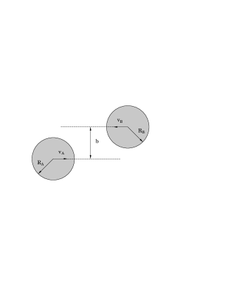
Figure 1: The schematic representation of the collision experiment. In all the simulations $R_{A}=R_{B}$ and $\vec{v}_{A}=-\vec{v}_{B}$ were chosen.

The schematic representation of the experimental situation can be seen in Fig. 1. In the simulations all the microscopic parameters of the model shown in Table 1 were fixed, only the macroscopic parameters were varied, i.e. the initial velocities $\vec{v}_{A},\vec{v}_{B}$ and the radii $R_{A},R_{B}$ of the colliding particles and the impact parameter $b$. Only the monodisperse case $R_{A}=R_{B}$ was considered. The velocities of the two particles have the same magnitude and opposite direction $\vec{v}_{A}=-\vec{v}_{B}$. The impact parameter $b$ is defined as the distance between the two centers of mass in the direction perpendicular to the velocity vectors. $b$ can vary in the interval $[0,R_{A}+R_{B}]$. The range of the initial velocities was chosen to be $12.5-50m/s$, and that of the radii $5-15cm$.

In the following the results are presented concerning the time evolution of the fragmenting system, the spatial distribution of the fragments, the distribution of the fragment velocities and of the fragment mass.

3.1 Fragmentation process

In Ref.  4, based on detailed experimental studies, the low - velocity impact phenomena of solid spheres were classified into five categories: $(1)$ elastic rebound, $(2)$ rebound with contact damage, $(3)$ rebound with longitudinal splits, $(4)$ destruction with shatter- cone like fragments, and $(5)$ complete destruction. These categories can be well distinguished by the imparted energy. Our simulations cover the $4th$ and the $5th$ classes varying the initial velocities, the radii and the impact parameter. Results about the $1st$ case will be presented in a forthcoming publication.

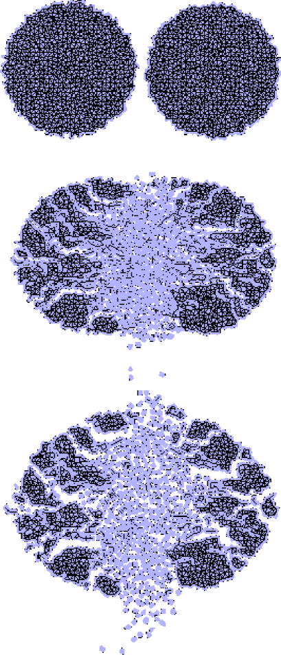
Figure 2: The central collision ($b=0$) of two discs of equal size $R=15cm$ at $v=25m/s$ velocity. Snapshots of the evolving system present the initial configuration, an intermediate state and the final breaking scenario.

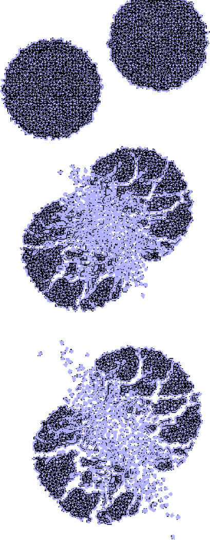
Figure 3: The collision of two discs of equal size at $b/d=0.5$. All the parameters are as in Fig. 2 and the snapshots are also taken at the same times.

The collision initiates with the contact of the two bodies. At our velocity range it can be assumed that the impact proceeds quasi-statically since the impact velocity is much smaller than the velocity of the generated shock wave. Fig. 2 and Fig. 3 show representative examples of the time evolution of the colliding system at $b/d=0$ (central collision) and $b/d=0.5$, respectively. Here $d$ denotes the diameter of the particles. Due to the high compression a strongly damaged region is formed around the impact site, where practically all the beams are broken and all the fragments are single polygons. Since the beam breaking dissipates energy the growth of the damage stops after some time. The shock wave reaching the free boundary gives rise to the expansion of the particles. This overall expansion initiates crack formation which results in the final fragmentation of the solids. The fragments at the anti - impact site of the particles are larger and they mainly have a shatter cone like shape in agreement with experimental observations[4]. Due to the geometry of the system, the fine fragments in the contact zone are confined unless the global expansion sets in. Thus they undergo many secondary collisions while the fragments formed in the outer region can escape without further interaction. This has an important effect on the velocity distribution of the debris in the final state. (See Chapter  3.2.)

Since the impact velocity is much smaller than the sound speed of the material, the peak stress produced by the collision around the impact site is proportional to the normal component of the impact velocity $v_{n}$ with respect to the contact surface. That is why the final breaking scenarios strongly depend on the impact parameter. In Fig. 2, in the case of a central collision the damage is larger, i.e. the shattered zone is larger and the average fragment size is smaller than in Fig. 3. The larger $b/d$ (the smaller $v_{n}$), the less energy is converted into breaking and the more energy is carried away by the motion of the fragments.

In the expanding system the fragments are not isotropically distributed but the fragment ejection has a preferred direction depending also on the impact parameter. In Fig 4 the jet-like structure of the fragment ejection can be observed, which means that most of the fragments are flying in two “cones” having a common axis and a relatively small opening angle.

To determine the jet-axis we calculated the sphericity $S$ of the velocity distribution:

$$S=\min_{\vec{n}}2\frac{\sum v_{Ti}^{2}}{\sum v_{i}^{2}},$$ (2)

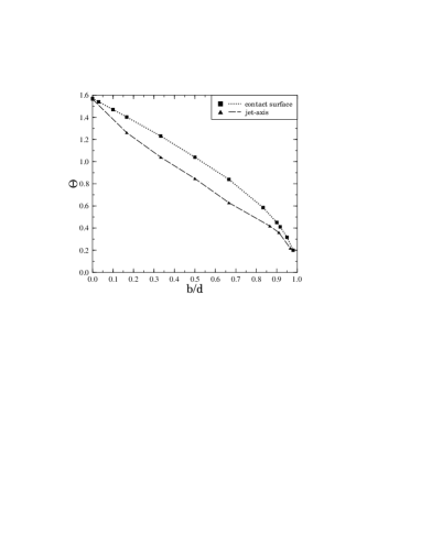
Figure 5: The angle of the jet-axis and that of the contact surface with respect to the direction of the initial velocity as a function of $b/d$.

where $\vec{v}_{i}$ is the velocity of the center of mass of fragment $i$ and $v_{Ti}$ is its transversal component with respect to $\vec{n}$. The factor $2$ scales the upper limit of $S$ to 1 in the case of the isotropic velocity distribution. The jet-axis $\vec{n}^{*}$ minimizes the above expression. The angle of the jet-axis and that of the contact surface with respect to the direction of the initial velocity as a function of $b/d$ are shown in Fig. 5.

Because of the low impact velocity there is enough time for stress rearrangement inside the two bodies. Thus the stress can have a tangential direction to the contact surface giving rise to the jet-like ejection. (A detailed study of the stress field inside disc shaped particles due to an impact will be presented in the forthcoming publication mentioned above.) This argument is also supported by the fact that the long cracks passing through the solids are either perpendicular to the contact zone or they go radially to the surface of the solids. For the central and peripheric collisions the jet-axis is practically parallel to the contact surface (see Fig.5). The two curves differ considerably only at intermediate $b$ values.

The angular distribution of the fragments around the direction of the initial velocity is shown in Fig. 6. The concentration of the debris in a small solid angle can be observed. The position of the peak of the distributions practically coincides with the jet-axis.

3.2 Scaling of the velocity distribution

In order to study the velocity distribution of the fragments we performed two sets of simulations alternatively fixing the initial velocity and the radius of the particles changing the value of the other one. Only central collisions $b/d=0$ were considered. In both cases the distribution of the $x$ and $y$ components of the velocity of the center of mass of the fragments was evaluated. The $x$ axis was chosen to be parallel to the initial velocity of the collision.

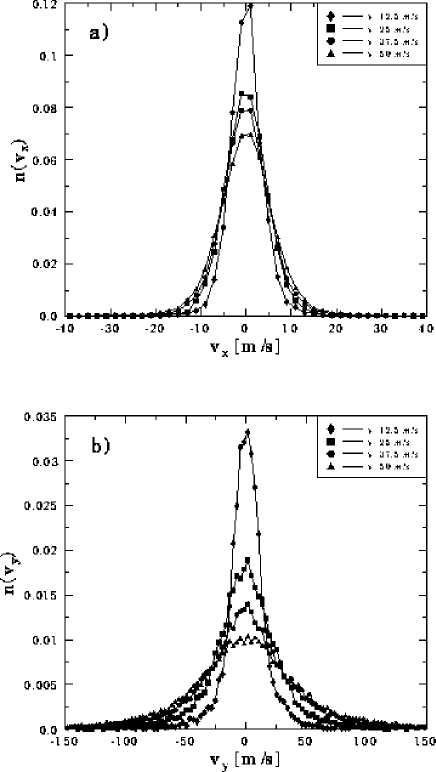
Figure 7: The distribution of the $x$ and $y$ components of the velocity of the fragments with fixed system size $R=15cm$ varying the initial velocity $v$.

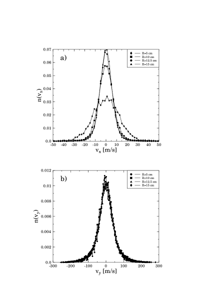
Figure 8: The distribution of the $x$ and $y$ components of the velocity of the fragments with fixed initial velocity $v=50m/s$ varying the radius $R$ of the particles.

Fig. 7 and Fig. 8 show the results for fixed $R=15cm$ varying the initial velocity and for fixed $v=50m/s$ varying the radius of the particles, respectively. One can observe that the distributions of both velocity components always exhibit a Gaussian form. The zero mean value is a consequence of momentum conservation. In the $x$ direction the fragments are slower, i.e. the values of $v_{x}$ are much smaller than those of $v_{y}$. There is a small fraction of the debris, which has velocity larger than the initial one, in agreement with experimental results[5].

For fixed system size $R$ one can see that the increasing initial velocity $v$ results in a larger dispersion of the fragment velocities, increasing the deviation of the distributions $n(v_{x})$, $n(v_{y})$ as shown in Fig. 7. For fixed initial velocity in Fig. 8 the deviation of $n(v_{x})$ is decreasing with increasing system size but it remains constant for $n(v_{y})$. The scaling analysis of the velocity distributions is of major interest. By appropriately rescaling the axes one can collapse the data obtained at fixed values of the macroscopic parameters onto one single curve. We denote the velocity components by $v_{i}$, where $i=(x,y)$. The data collapse can be obtained using the same form of scaling ansatz for both data sets:

$$n(v_{i}) = R^{\alpha_{i}}\phi(v_{i}R^{\alpha_{i}})\hskip 28.45274pt\mbox{ for fixed }v,$$ (3)

$$n(v_{i}) = v^{\beta_{i}}\psi(v_{i}v^{\beta_{i}})\hskip 35.56593pt\mbox{ for fixed }R,$$ (4)

where $\phi,\psi$ are scaling function and $\alpha_{i},\beta_{i}$ are the scaling exponents belonging to the velocity component $v_{i}$. In principle, one could introduce two different exponents for the macroscopic variables within Eqs. (3, 4) but in our case they turned to be equal within the error bars. The values of $\alpha_{i}$ and $\beta_{i}$ are presented in Table 2.

Table 2: The values of the scaling exponents $\alpha_{i},\beta_{i}$ for $n(v_{x})$, $n(v_{y})$.

	$\alpha_{i}$	$\beta_{i}$
$n(v_{x})$	$-0.7\pm 0.05$	$0.35\pm 0.04$
$n(v_{y})$	$0\pm 0.02$	$0.85\pm 0.05$

Note, that in both cases the scaling exponents of the two velocity components $\alpha_{x},\alpha_{y}$ and $\beta_{x},\beta_{y}$ are significantly different.

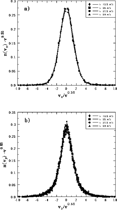
Figure 9: Scaling of the velocity distributions for fixed system size $R=15cm$ varying the initial velocity $v$.

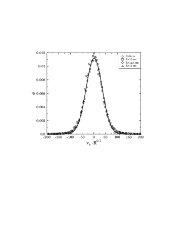
Figure 10: Scaling of the velocity distributions for fixed initial velocity $v=50m/s$ varying the radius $R$ of the particles. The solid line shows the Gaussian fit according to Eq. (5) for the scaling function $\phi$.

The data collapse obtained using Eqs. (3, 4) is illustrated by Figs. 9, 10. The quality of the collapse is satisfactory, there are fluctuation only for the smallest initial velocity in Fig. 9 and for the smallest radius in Fig. 10 when the number of fragments is not large enough. The scaling functions $\phi,\psi$ are the same for the two velocity components within the accuracy of the calculation. The scaling structure found implies that the distributions $n(v_{i})$ are Gaussians, the standard deviation $\sigma_{i}$ of which has a power law dependence on the macroscopic parameters, i.e.:

$$n(v_{i}) = \frac{1}{\sqrt{2\pi}\sigma_{i}}\exp{\left[-\frac{1}{2}\left(\frac{v_{i}}{\sigma_{i}}\right)^{2}\right]},$$ (5)

$$\sigma_{i}(R,v) \sim R^{\alpha_{i}}v^{\beta_{i}}.$$ (6)

Fig. 10 shows a representative example of the Gaussian fit too. Eq. (5) was fitted to the scaling function $\phi$.

The shape of the velocity distribution of the fragments is mainly determined by the stress distribution in the bodies just before the breaking of the beams. When, due to the geometry of the system, energetic fragments are confined during some time, secondary collisions of the products can also have a considerable contribution. In our case this effect can be responsible for the Gaussian shape.

The deviations of the two velocity components $\sigma_{x}$ and $\sigma_{y}$ can be considered as the linear extensions of the fragment jet in the velocity space in the $x$ and $y$ directions. Their ratio $s$ is a characteristic quantity of the jet shape. (Note, that here we considered solely central collisions. The above argument can be generalized to non-central collisions choosing the $x$ direction perpendicular to the jet-axis.) Eq. (6) yields the dependence of $s$ on the macroscopic parameters:

$$s(R,v)=\frac{\sigma_{y}}{\sigma_{x}}\sim R^{\alpha_{y}-\alpha_{x}}v^{\beta_{y}-\beta_{x}}=R^{\gamma}v^{\delta}$$ (7)

The value of the new exponents characterizing the jet-shape are $\gamma=0.7\pm 0.05$ and $\delta=0.5\pm 0.05$.

It is generally believed that once a solid, e.g. asteroid suffers catastrophic destruction the pieces fly apart from each other in all directions. However this scheme is not necessarily true. From our treatment it follows that we have anisotropic clustering of fragments, i.e. most of the fragment velocities are much smaller than the impact velocity and the particles fly in rather collimated jets, the shape of which is described by $\gamma$ and $\delta$. This can have important consequences for the later evolution of the fragmented system. For instance, in the case of the collision of asteroids fragments could recombine due to mutual gravitation forming a cloud-like object.

3.3 The fragment mass distribution

Beside the fragment velocities, the mass distribution of the debris also has practical importance. Fig. 2 and Fig. 3 show that the contact zone around the impact site gives the main contribution to the small fragments while the larger ones are dominated by the anti-impact site. This detachment effect becomes more pronounced for smaller collision velocities when the type of the impact passes from class $(5)$ to $(4)$ (see Chapter  3.1).

The fragment mass histograms $F(m)$ are presented in Figs. 11, 12 for fixed system size and for fixed initial velocity, respectively. Here $F(m)$ denotes the number of fragments with mass $m$ divided by the total number of fragments. In order to obtain the correct shape of the distributions at the coarse products as well as at the finer ones logarithmic bining was used, i.e. the bining is equidistant on logarithmic scale. The histograms have two cutoffs. The lower one is due to the existence of single unbreakable polygons (smallest fragments) and the upper one is given by the finite size of the system (largest fragment).

In Fig. 11 the histogram belonging to the smallest collision velocity has two well distinguished local maxima, one for the fine fragments (single polygons and pairs) and another one for the large pieces, which are comparable to the size of the colliding particles. In between, for the “Intermediate Mass Fragments” (IMF) $F(m)$ shows power law behavior, i.e. we seem to have:

$$F(m)\sim m^{-\mu}.$$ (8)

The effective exponent $\mu$ was obtained from the estimated slope of the curve, $\mu=2.1\pm 0.05$ for $v=12.5m/s$. At low impact velocity this shape of distribution is characteristic for light-fragment ejection from a heavy system[9]. As the initial velocity increases the peak of the heavy fragments gradually disappears giving rise to an increase of the contribution of IMFs, while the fraction of the shattered products hardly changes. In the IMF region the slope of $F(m)$ depends slightly on the impact velocity, i.e. the distributions become less steep with increasing $v$. The straight line in Figs. 11, 12 shows the power law fitted at our highest velocity $v=50m/s$ and for $R=15cm$ with exponent $\mu=1.75\pm 0.05$.

For fixed initial velocity the histograms belonging to different system sizes are characterized practically by the same exponent $\mu=1.75\pm 0.05$ as shown in Fig. 12. Only in the case of the smallest system, which suffers catastrophic destruction shattering the particles completely, the exponent is larger.

It is important to note that in nuclear fragmentation experiments of gold projectile with several targets, the charge distribution of the fragments shows a similar dependence on the deposited energy of the collision[25].

Beside the size distribution of the debris there is also interest in the energy required to achieve a certain size reduction. It was revealed in collision experiments[4] that the mass of the largest fragment $M_{max}$ normalized by the total mass $M_{tot}$ follows a power law as a function of the specific energy, i.e. the ratio of the imparted energy $E$ and the total mass of the system. The exponent characterizing the size reduction seems to be independent of the type of the material but it is sensitive to the shape of the colliding particles. For spherical bodies it was found to be around $0.7$, while for cubic systems around $1.5$ (see Ref. 4). Note, that in Fig. 12 the fixed initial velocity implies that the specific energy is also constant. This results in more or less the same value of $M_{max}/M_{tot}$ for the different curves. In Fig. 11 for fixed system size the specific energy varies with the initial velocity resulting change of $M_{max}/M_{tot}$.

In order to obtain more information about the size reduction we performed a set of simulations on the $32$ partition of the CM5 with fixed $R=15cm$ particle radius changing the initial velocity within the interval $12.5-50m/s$ in 32 steps. In Fig. 13 $M_{max}/M_{tot}$ is plotted against the specific energy $E/M_{tot}$ on double logarithmic scale. Although the data are rather scattered a power law seems to be a reasonable fit with exponent $0.68$ in agreement with the experimental results.

4 Conclusion

We have studied the low velocity impact phenomena of two solid discs of the same size using our cell model[20]. We focused our attention on the spatial distribution of the debris and on the analysis of the fragment velocities and fragment mass.

Anisotropic clustering of fragments was revealed, which manifests in the jet structure of the fragment ejection. Due to the anomalous scaling of the distributions of the velocity components the jet-shape can be characterized by two independent exponents. The mass distribution of the intermediate mass fragments shows a power law behavior, whose exponent slightly decreases with increasing imparted energy. We have noted that the charge distributions obtained in nuclear multifragmentation experiments show a similar dependence on the deposited energy of the collision. This is a manifestation of the independence of the global quantities of the fragmenting system from the microscopic details of the mechanism of the individual breaking.

The mass of the largest fragment normalized by the total mass also follows a power law as a function of the imparted energy density with exponent close to the experimental observations.

Still our study makes a certain number of technical simplifications which might be important for a full quantitative grasp of fragmentation phenomena. Most important seems to us the restriction to two dimensions, which should be overcome in future investigations. The existence of elementary, non-breakable polygons restricts fragmentation on lower scales and hinders us from observing the formation of a powder of a shattering transition[16].

Experiments showed[4] that the relative size of the colliding bodies is an important parameter describing the low velocity impact phenomena if the mechanical properties of the bodies are the same. In the future our studies should be extended to this polydisperse case too.

Figure 4: The velocity vectors of the center of mass of the fragments for three different impact parameters. One can observe the jet structure of the fragment ejection. All the parameters are as in Fig. 2.

Figure 6: The angular distribution of the fragments around the direction of the initial velocities for different impact parameters.

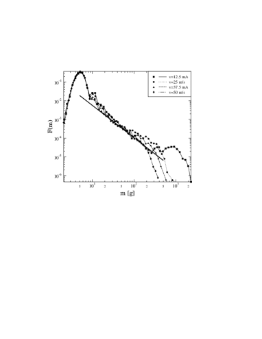
Figure 11: The fragment mass histograms for fixed system size $R=15cm$ varying the initial velocity $v$. The straight line shows the power law fitted to the curve belonging to $v=50m/s$.

Figure 12: The fragment mass histograms for fixed initial velocity $v=50m/s$, varying the system size $R$. The straight line is the same as in Fig. 11.

Figure 13: The mass of the largest fragment normalized by the total mass as a function of the specific energy.

References

- [1] D. L. Turcotte, J. of Geophys. Res. Vol. 91 B2, 1921 (1986).
- [2] C. Thornton, K. K. Yin and M. J. Adams, J. Phys. D. Appl. Phys. 29, 424 (1996)
- [3] N. Arbiter, C. C. Harris and G. A. Stamboltzis, Soc. of Min. Eng. 244, 119 (1969).
- [4] T. Matsui, T. Waza, K. Kani and S. Suzuki, J. of Geophys. Res. 87 B13, 10968 (1982).
- [5] A. Fujiwara and A. Tsukamoto, Icarus 44, 142 (1980).
- [6] M. Matsushita and T. Ishii, Fragmentation of long thin glass rods, Department of Physics, Chuo University (1992).
- [7] L. Oddershede, P. Dimon, and J. Bohr, Phys. Rev. Lett. 71, 3107 (1993).
- [8] A. Meibom and I. Balslev, Phys. Rev. Lett. 76, 2492 (1996)
- [9] D. Beysens, X. Campi, E. Pefferkorn (eds), Fragmentation Phenomena, World Scientific 1995.
- [10] R. Botet and M. Ploszajczak, in Ref. [9]
- [11] M. Matsushita and K. Sumida, How do thin glass rods break? (Stochastic models for one - dimensional fracture), Chuo University, Vol. 31, pp. 69-79 (1981).
- [12] M. Marsili and Y. C. Zhang, preprint
- [13] P. L. Krapivsky and E. B. Naim, Phys. Rev. E 50 3502 (1995).
- [14] G. Hernandez, H. J. Herrmann, Physica A 215, 420 (1995).
- [15] S. Steacy and C. Sammis, An automaton for fractal patterns of fragmentation, Nature 353 250 (1991).
- [16] S. Redner, in: Statistical Models for the Fracture of Disordered Media (North Holland, Amsterdam, 1990).
- [17] H. Inaoka, H. Takayasu, preprint.
- [18] A. V. Potapov, M. A. Hopkins and C. S. Campbell, Int. J. of Mod. Phys. C 6, 371 (1995).
- [19] A. V. Potapov, M. A. Hopkins and C. S. Campbell, Int. J. of Mod. Phys. C 6, 399 (1995).
- [20] F. Kun and H. J. Herrmann, preprint cond-mat/9512017
- [21] H. J. Tillemans, H. J. Herrmann, Physica A 217, 261 (1995).
- [22] K. B. Lauritsen, H. Puhl and H. J. Tillemans, Int. J. of Mod. Phys. C 5, 909 (1994).
- [23] H. J. Herrmann and S. Roux (eds.) Statistical Models for the Fracture of Disordered Media (North Holland, Amsterdam, 1990).
- [24] H. J. Herrmann, A. Hansen, S. Roux, Phys. Rev. B 39, 637 (1989).
- [25] C. A. Ogilvie et al, Phys. Rev. Lett. 67, 1214 (1991)