Statistical mechanics of a correlated energy landscape model for protein folding funnels

Abstract

Energetic correlations due to polymeric constraints and the locality of interactions, in conjunction with the apriori specification of the existence of a particularly low energy state, provides a method of introducing the aspect of minimal frustration to the energy landscapes of random heteropolymers. The resulting funnelled landscape exhibits both a phase transition from a molten globule to a folded state, and the heteropolymeric glass transition in the globular state. We model the folding transition in the self-averaging regime, which together with a simple theory of collapse allows us to depict folding as a double-well free energy surface in terms of suitable reaction coordinates. Observed trends in barrier positions and heights with protein sequence length, stability, and temperature are explained within the context of the model. We also discuss the new physics which arises from the introduction of explicitly cooperative many-body interactions, as might arise from side-chain packing and non-additive hydrophobic forces. Denaturation curves similar to those seen in simulations are predicted from the model.

I Introduction

Molecular scientists view protein folding as a complex chemical reaction. Another fruitful analogy from statistical physics is that folding resembles a phase transition in a finite system. A new view of the folding process combines these two ideas along with the notion that a statistical characterization of the numerous possible protein configurations is sufficient for understanding folding kinetics in many regimes.

The resulting energy landscape theory of folding acknowledges that the energy surface of a protein is rough, containing many local minima like the landscape of a spin glass. On the other hand, in order to fold rapidly to a stable structure there must also be guiding forces that stabilize the native structure substantially more than other local minima on the landscape. This is the principle of minimum frustration [1]. The energy landscape can be said then to resemble a “funnel”. [2] Folding rates then depend on the statistics of the energy states as they become more similar to the native state at the bottom of the funnel.

One powerful way of investigating protein energy landscapes has been the simulation of “minimalist” models. These models are not fully atomistic, but caricature the protein as a series of beads on a chain either embedded in a continuum [3] or on a lattice [4]. A correspondence, in the sense of phase transition theory, between these models and real proteins has been set up using energy landscape ideas [5]. Many issues remain to be settled however in understanding how these model landscapes and folding mechanisms change as the system under study becomes larger and as one introduces greater complexity into the modelling of this correspondence, as for example, by explicitly incorporating many-body forces and extra degrees of freedom. Simulations become cumbersome for such surveys, and an analytical understanding is desirable.

Analytical approaches to the energy landscape of proteins have used much of the mathematical techniques used to treat spin glasses [6] and regular magnetic systems [7]. The polymeric nature of the problem must also be taken into account. Mean field theories based on replica techniques [8] and variational methods [9] have been very useful, but are more difficult to make physically intuitive than the straightforward approach of the random energy model [10], which flexibly takes into account many of the types of partial order expected in biopolymers [11]. Recently we have generalized the latter approach to take into account correlations in the landscape of finite-sized random heteropolymers [12]. This treatment used the formalism of the generalized random energy model (GREM) analyzed by Derrida and Gardner [13]. In this paper, we extend that analysis to take into account the minimum frustration principle and thereby treat protein-like, partially non-random heteropolymers.

There are various ways of introducing the aspect of minimum frustration to analytical models with rugged landscapes. One way recognizes that many empirical potentials actually are obtained by a statistical analysis of a database, and when the database is finite, there is automatically an aspect of minimal frustration for any member of that database. Thus the so-called “associative memory” hamiltonian models [14] have co-existing funnel-like and rugged features in their landscape. Other methods of introducing minimal frustration model the process of evolution as giving a Boltzmann distribution over sequences for an energy gap between a fixed target structure and unrelated ones [15]. All of the above approaches can be straightforwardly handled with replica-based analyses. Here we show that the GREM analyses can be applied to minimally frustrated systems merely by requiring the energy of a given state to be specified as having a particularly low value. Minimally frustrated, funnelled landscapes are just a special case of the general correlated landscape studied earlier.

A convenient aspect of the correlated landscape model is that it allows the treatment of the polymer physics in a very direct way, using simple statistical thermodynamics in the tradition of Flory [16]. Here we will show how the interplay of collapse and topological ordering can be studied. In order to do this we introduce a simple “core-halo” model to take into account the spatially inhomogenous density. We will also discuss the role of many-body forces in folding. Explicitly cooperative many-body forces have often been involved in the thinking about protein structure formation. Hydrophobic forces are often modelled as involving buried surface area. Such an energy term is not pairwise-additive but involves three or more interacting bodies. Side-chain packing involves objects fitting into holes created by more than one other part of the chain, thus the elimination of side-chains from the model can yield an energy function for backbone units with explicit non-additivity. These many-body forces can be treated quite easily by the GREM, and we will see that they can make qualitative changes in the funnel topography.

To illustrate the methods here, we construct two-dimensional free energy surfaces for the folding funnel of minimally frustrated polymers. These explicitly show the coupling between between density and topological similarity in folding. We pay special attention to the location of the transition state ensemble and discuss how this varies with system size, cooperativity of interactions, and thermodynamic conditions. In the case of the $27$-mer on a lattice, a detailed fit to the lattice simulation data [4] is possible. Although delicate cancellations of energetic and entropic terms are involved in the overall free energy, plausible parameters fit the data.

The trends we see in the present calculations are very much in harmony with the experimental information on the nature and location of the transition state ensemble [17, 18]. We intend later to return to this comparison, especially taking into account more structural details within the protein.

The organization of this paper is as follows: In Sec. 2 we introduce a theory of the free energy at constant density, and in this context investigate the effects of cooperative interactions on the transition state ensemble and corresponding free energy barrier. In Sec. 3 we detail a simple theory coupling collapse with topological similarity, and resulting in the “core-halo” model described there. In Sec. 4 we apply this collapse theory to obtain the free energy in terms of density and topological order, now coupled via the core-halo model. In the same section we compare our model of the minimally frustrated heteropolymer with lattice simulations of the $27$-mer. In terms of the categorization of Bryngelson et. al. [2] these free energy surfaces depict scenarios described as type I or type IIa folding. We then study the quantitative aspects of the barrier as a function of the magnitude of $3$-body effects. The dependence of position and height of the barrier as a function of sequence length is studied, as well as the effects of increasing the stability gap. Finally, we study the denaturation curve as determined by the constant and variable density models. In Sec. 6 we discuss the results and conclude with some remarks.

II A Theory of the Free Energy

In this section, we show how the apriori specification of the existence of a particularly low energy configuration, together with a theory of energy correlations for configurationally similar states, leads to a model for the folding transition and corresponding free energy surface in protein-like heteroplolymers. This ansatz for the correlated energy landscape corresponds to the introduction of minimal frustration in a random energy landscape, where the order parameter here (which will function as a reaction coordinate for the folding transition) counts the number of native contacts or hydrogen bonds.

The GREM theory for random heteropolymers developed by us earlier investigates the interplay between entropy loss and energetic roughness as a function of similarity to any given reference state, all at fixed density. However for exceptional reference states such as the ground state of a well-packed protein, the density is not independent of configurational similarity, so a theory of the coupling of density with topological similarity must also be developed (section 3).

We start by assuming a simple “ball and chain” model for a protein which is readily comparable with simulations, for example of the $27$-mer, which is widely believed to capture many of the quantitative aspects of folding (section 4). Proteins with significant secondary structure have an effectively reduced number of interacting units as may be described by a ball and chain model. Properties of both, when appropriately scaled by critical state variables such as the folding temperature $T_{\mbox{F}}$, glass temperature $T_{\mbox{G}}$, and collapse temperature $T_{\mbox{C}}$, will obey a law of corresponding states [5]. Thus the behavior describing a complicated real protein can be validly described by an order parameter applied to a minimal ball and chain model in the same universality class. For a $27$-mer on a 3-dimensional cubic lattice, there are $28$ contacts in the most collapsed (cubic) structure. For concreteness we take such a maximally compact structure to be the configuration of our ground state, the generalization to a less compact ground state being straightforward in the context of the model to be described. For a collapsed polymer of sequence length $N$, the number of pair contacts per monomer , $z_{\mbox{N}}$, is a combination of a bulk term, a surface term, and a lattice correction [19]. The effect of the surface on the number of contacts is quite important even for large macromolecules, as $z_{3}(N)$ approaches its bulk value of 2 contacts per monomer rather slowly, as $\sim 2-3N^{-1/3}$.

To describe states that are not completely collapsed, we introduce the packing fraction $\eta\cong N\sigma/R_{g}^{3}$ as a measure of the density of the polymer, where $\sigma$ is the volume per monomer and $R_{g}$ is the radius of gyration of the whole protein. So for less dense states the total number of contacts is reduced from its collapsed value $Nz_{\mbox{N}}$, to $Nz_{\mbox{N}}\eta$.

In the spirit of the lattice model we have in mind for concreteness, we introduce a simple contact hamiltonian to determine the energy of the system:

$${\cal H}=\sum_{i<j}\varepsilon_{ij}\sigma_{ij}\;,$$ (II.1)

where $\sigma_{ij}=1$ when there is a contact made between monomers $\left\{ij\right\}$ in the chain, and $\sigma_{ij}=0$ otherwise. Here contact means that two monomers $\left\{ij\right\}$, non-consecutive in sequence along the backbone chain, are adjacent in space at neighboring lattice sites. $\varepsilon_{ij}$ is a random variable so that, at constant density, the total energies of the various configurations, each the sum of many $\varepsilon_{ij}$, are approximately gaussianly distributed by the central limit theorem, with mean energy (at a given density $\eta$) $\overline{E_{\eta}}=Nz_{\mbox{N}}\eta\overline{\varepsilon}$, (where $\overline{\varepsilon}$ is simply defined as the mean energy per contact and $Nz_{\mbox{N}}\eta$ is again the total number of contacts), and variance $\Delta\!E^{2}_{\eta}=Nz_{\mbox{N}}\eta\varepsilon^{2}$, where $\varepsilon^{2}$ is the effective width of the energy distribution per contact.

Suppose there exists a configurational state $n$ of energy $E_{n}$ (which will later become the “native” state). Then if the Hamiltonian for our system is defined as in eq. (II.1), we can find the probability that configuration $a$ has energy $E_{a}$, given that $a$ has an overlap $Q_{an}$ with $n$, [12] where $Q_{an}\equiv Q$ is the number of contacts that state $a$ has in common with $n$, divided by the total number of contacts $Nz_{\mbox{N}}\eta$ (since this analysis is at constant density both $a$ and $n$ have $Nz_{\mbox{N}}\eta$ contacts). This distribution is simply a gaussian with a $Q$ dependent mean and variance:

$$\frac{P_{an}\left(E_{a}|Q|E_{n}\right)}{P_{n}\left(E_{n}\right)}\sim\exp\left(-\frac{\left[\left(E_{a}-\overline{E}\right)-Q\left(E_{n}-\overline{E}\right)\right]^{2}}{2Nz_{\mbox{N}}\eta\varepsilon^{2}\left(1-Q^{2}\right)}\right)$$ (II.2)

When $Q=1$ states $a$ and $n$ are identical and must then have the same energy, which (II.2) imposes by becoming delta function, and when $Q=0$ states $a$ and $n$ are uncorrelated and then (II.2) becomes the gaussian distribution of the Random Energy Model for the energy of state $a$ [1]. Expression (II.2) holds for all states of the same density as $n$, e.g. all collapsed states if $n$ is the native state (the degree of collapse must be a somewhat coarse-grained description to avoid fluctuations due to lattice effects coupled with finite size).

Previously a theory was developed of the configurational entropy $S_{\eta}\left(Q\right)$ as a function of similarity $Q$, at constant density $\eta$. [12] Given $S_{\eta}\left(Q\right)$ and the conditional probability distribution (II.2), the average number of states of energy $E$ and overlap $Q$ with state $n$, all at density $\eta$, is then

$$\left<\mbox{n}_{\eta}\left(E|Q|E_{n}\right)\right> = \mbox{e}^{S_{\eta}\left(Q\right)}\times\frac{P\left(E|Q|E_{n}\right)}{P\left(E_{n}\right)}$$ (II.3)

$$\sim \exp N\left\{s_{\eta}\left(Q\right)-\frac{1}{2\left(1-Q^{2}\right)}\left(\frac{\left(E-\overline{E}\right)-Q\left(E_{n}-\overline{E}\right)}{NJ_{\eta}}\right)^{2}\right\}$$ (II.4)

where $J_{\eta}^{2}\equiv z_{\mbox{N}}\eta\varepsilon^{2}$ and $s_{\eta}\left(Q\right)\equiv S_{\eta}\left(Q\right)/N$ [20]. Equation (II.4) is still gaussian with a large number of states provided $E<E_{c}$ (for negative energies) where $E_{c}=QE_{n}+NJ_{\eta}\sqrt{2\left(1-Q^{2}\right)s_{\eta}\left(Q\right)}$ is a critical energy below which the exponent changes sign and the number of states becomes negligably small.

At temperature $T$, the Boltzmann factor $\frac{1}{Z}e^{-E/T}$ [21] weighting each state shifts the number distribution of energies so that the maximum of the thermally weighted distribution can be interpreted as the most probable (thermodynamic) energy at that temperature

$$E_{\eta}\left(T,Q,E_{n}\right)=\overline{E}+Q\left(E_{n}-\overline{E}\right)-\frac{Nz_{\mbox{N}}\eta\varepsilon^{2}\left(1-Q^{2}\right)}{T}\;.$$ (II.5)

The above expression for the most probable energy is useful provided the distribution (II.4) is a good measure of the actual number of states at $E$ and $Q$, the condition for which is that the fluctuations in the number of states be much smaller than the number of states itself. To this end, we make here the simplifying assumption that in each “stratum” defined by the set of states which have an overlap $Q$ with the native state, the states themselves are not further correlated with each other, i.e. $P\left(E_{a},Q,E_{b},Q|E_{n}\right)=P\left(E_{a},Q,E_{n}\right)P\left(E_{b},Q,E_{n}\right)$, so that in each stratum of the reaction coordinate $Q$, the set of states is modelled by a random energy model. Then since the number of states $\mbox{n}_{\eta}\left(E|Q|E_{n}\right)$ counts a collection of random uncorrelated variables, large when $E>E_{c}$, the relative fluctuations $\sqrt{\left<\left(n-\left<n\right>\right)^{2}\right>}/\left<n\right>$ are $\sim\left<n\right>^{-1/2}$ and are thus negligible. So $n\left(E|Q|E_{n}\right)\approx\left<n\left(E|Q|E_{n}\right)\right>$, and we can evaluate the exponent in the number of states (II.4) at the the most probable energy (II.5) as an accurate measure of the ($Q$ dependent) thermodynamic entropy at temperature $T$

$$S_{\eta}\left(T,Q,E_{n}\right)=S_{\eta}\left(Q\right)-\frac{Nz_{\mbox{N}}\eta\varepsilon^{2}\left(1-Q^{2}\right)}{2T^{2}}\;.$$ (II.6)

The assumption of a REM at each stratum of $Q$ is clearly a first approximation to a more accurate correlational scheme. The generalization to treat each stratum itself as a GREM as in our earlier work is nevertheless straightforward, since our earlier work suggested only quantitative changes, which we will not pursue here. If two configurations $a$ and $b$ have overlap $Q$ with state $n$ and thus are correlated to $n$ energetically, they are certainly correlated to each other, particularly for large overlaps where the number of shared contacts is large. Using the REM scheme at each stratum is more accurate for small $Q$ and breaks down to some extent for large $Q$. In the ultrametric scheme of the GREM, states $a$ and $b$ have an overlap $q_{ab}\geq Q$, which is more accurate for large overlap than at small $Q$ where states $a$ and $b$ need not share any bonds and still can both have overlap $Q$ with $n$. One can also further correlate the energy landscape of states by stratifying with respect to $q_{ab}=q$ and so on, resulting in a hierarchy of overlaps and correlations best treated using renormalization group ideas.

Just as the number of states (II.4) has a characteristic energy for which it vanishes, the REM entropy for a stratum at $Q$ (II.6) vanishes at a characteristic temperature

$$\frac{T_{g}\left(Q\right)}{\varepsilon}=\sqrt{\frac{z_{\mbox{N}}\eta\left(1-Q^{2}\right)}{2s_{\eta}\left(Q\right)}}$$ (II.7)

which signals the trapping of the polymer into a low energy conformational state within the stratum characterized by $Q$.

If $T_{g}(Q)$ is a monotonically decreasing function of $Q$, as the temperature is lowered the polymer will gradually be thermodynamically confined in its conformational search to smaller and smaller basins of states. The basin around the native state is the largest basin with the lowest ground state, and hence is the first basin within which to be confined. Its characteristic size at temperature $T$ is just the number of states within overlap $Q_{o}(T)$, where $Q_{o}(T)$ is the value of overlap $Q$ that gives $T_{g}(Q_{o})=T$ in equation (II.7). Thus there is now no longer a single glass temperature at which ergodic confinement suddenly occurs, as in the REM, but there is a continuum of basin sizes to be localized within at corresponding glass temperatures for those basins.

If $T_{g}(Q)$ has a single maximum at say $Q^{\star}$, the glass transition is characterized by a sudden REM-like freezing to a basin of configurations whose size is determined by $Q^{\star}$. The range of glass temperatures will turn out to be lower than the temperature at which a folding transition occurs (see Fig. 3), so that this model predicts a protein-like heteropolymer whose folded state is stable by several $k_{\mbox{B}}T$ at temperatures where freezing becomes important. A replica-symmetric analysis of the free energy is therefore sufficient to describe the folding transition to such deep native states that are minimally frustrated.

From the thermodynamic expressions for the energy (II.5) and entropy (II.6) with the mean energy at density $\eta$, we can write down the free energy per monomer above the glass temperature as the sum of 4 terms

$$\frac{F_{\eta}}{N}\left(T,Q,E_{n}\right)=z_{\mbox{N}}\eta\overline{\varepsilon}+Qz_{\mbox{N}}\delta\varepsilon_{\mbox{n}}-Ts_{\eta}\left(Q\right)-\frac{z_{\mbox{N}}\eta\varepsilon^{2}}{2T}\left(1-Q^{2}\right)\;,$$ (II.8)

where $z_{\mbox{N}}\delta\varepsilon_{n}=z_{\mbox{N}}(\varepsilon_{n}-\overline{\varepsilon})=\left(E_{n}-\overline{E}\right)/N$ is the extra energy for each bond beyond the mean homopolymeric attraction energy (the energy “gap” between an average molten globule structure and the minimally frustrated one), times the number of bonds per monomer, and $s_{\eta}\left(Q\right)=S_{\eta}\left(Q\right)/N$ is the entropy per monomer.

The first term in (II.8) multiplied by $N$ is just the homopolymeric attraction energy between all the monomers, for a polymer of density $\eta$. It depends only on the degree of collapse, and not on how many contacts are native contacts. The second term is the average extra bias energy if a contact is native, times the average number of native contacts per monomer. The third term measures the equilibrium bias towards larger configurational entropy at smaller values of the reaction coordintate $Q$. The last term accounts for the diversity of energy states that exist on a rough energy landscape, the variance of which lowers thermodynamically the energy more than the entropy, and so lowers the equilibrium free energy.

For a special surface in $\left(\delta\varepsilon_{\mbox{n}},\varepsilon,T\right)$ space, expression (II.8) has a double minimum structure in the reaction coordinate $Q$, with one entropic minimum at low $Q$ corresponding to the “molten globule” state, separated by a barrier from an energetic minimum at high $Q$ corresponding to a “folded” state. For a given temperature, values of $\delta\varepsilon_{\mbox{n}}$ and $\varepsilon^{2}$ can be obtained which are reasonably close to the values obtained by a more accurate analysis which includes the coupling of density with topology, but we will not examine the constant density case in much detail for reasons discussed below, except to remark that 1.) The true coupling between density and $Q$-constraints need not be strong to obtain a double-well free energy structure, 2.) For monomeric units with pair interactions, the molten globule and folded minima are not at $Q=0$ and $1$ respectively. The position of the molten globule state is near the maximum of the entropy of the system, which is at $Q\cong 0.1$ for the $27$-mer due to the interplay of confinement effects and the combinatorial mixing entropy inherent in the “coarse-grained” description $Q$. [12] The native minimum shifts to $Q=1$ when many-body interactions are introduced (see the next section ). 3.) The barrier height, at position $Q^{\circ}\cong 0.25$ for the $27$-mer with protein-like parameters ($T_{\mbox{F}}/T_{\mbox{G}}\cong 2$), is small ($\Delta F^{\circ}\approx k_{\mbox{B}}T_{\mbox{F}}$), due to the effective cancellation of entropy loss by negative energy gain, as the system moves toward the native state (This cancellation is reduced when many-body forces are taken into account). 4.) When a linear form for the entropy is used in equation (II.8), e.g. $s(Q)=s_{o}(1-Q)$ instead of the more accurate $s(Q)$ obtained in reference [12], the double minimum structure disappears and is replaced by a single minimum near $T_{\mbox{F}}$ at $Q\approx 1/2$, with the $Q=0$ and $Q=1$ states becoming free energy maxima. So folding is downhill or spinodal-like in this approximation.

A Effects of cooperative interactions

As the interactions between monomeric segments become more explicitly cooperative, the energetic correlations between states become significant only at greater similarity, with the system approaching the REM limit for $\infty$-body interactions, where the statistical energy landscape assumes a rough “golf-course” topography with a steep funnel close to the native state.

In the presence of many-body interactions, the homopolymer collapse energy also scales as a higher power of density ($\sim\overline{\varepsilon}\,\overline{z}^{m-1}$). For even moderate $m\sim{\cal{O}}\left(1\right)$ a first-order phase transition to collapsed states results, which effectively confines all reaction paths in the coordinate $Q$ between molten globule and folded states to those where the density is constant and $\approx 1$. So within this constant density approximation we can investigate the nature of the folding transition as a function of the cooperativity of the interactions, and see how the correlated landscape simplifies to the REM in the limit of $m$-body interactions with large $m$.

In the presence of $m$-body interactions, the $Q$ dependence in the pair energy distribution (II.2) scales with $Q$ as $Q^{m-1}$. Using this modified pair distribution along with the collapsed homopolymeric state as our zero point energy, the free energy (II.8) becomes

$$\frac{F}{N}\left(T,Q,E_{n}\right)=-Ts_{1}\left(Q\right)-Q^{m-1}z_{\mbox{N}}\left|\delta\varepsilon_{\mbox{n}}\right|-\frac{z_{\mbox{N}}\varepsilon^{2}}{2T}\left(1-Q^{2\left(m-1\right)}\right)\;,$$ (II.9)

where $s_{1}\left(Q\right)$ is the entropy as a function of constraint $Q$ for a fully collapsed polymer. For pure $3$-body interactions and higher, the globule and folded states are very nearly at $Q\cong 0$ and $Q\cong 1$ respectively (see figure 1A). To the extent that this approximation is good, we can equate the free energies of the molten globule and folded structures and obtain an $m$-independent folding temperature (note again that this is not a good approximation for pair interactions):

$$T_{\mbox{F}}=\frac{z_{\mbox{N}}\left|\delta\varepsilon_{\mbox{n}}\right|}{2s_{o}}\left(1+\sqrt{1-\frac{2s_{o}\varepsilon^{2}}{z_{\mbox{N}}\delta\varepsilon_{\mbox{n}}^{2}}}\right)$$ (II.10)

where $s_{o}$ is the maximum of the entropy as a function of constraint $Q$ (essentially the $\log$ of the total number of configurations).

From expression (II.10) we can obtain a first approximation to the constraint on the magnitude of the gap energy $\delta\varepsilon_{\mbox{n}}$ in order to have a global folding transition (rather than merely a local glass transition) to the low energy state in question. The condition that the square root term in eq. (II.10) be real gives the minimum gap for global foldability in terms of the roughness $\varepsilon$:

$$\frac{\delta\varepsilon_{\mbox{n}}^{\left(c\right)}}{\varepsilon}=\sqrt{\frac{2s_{o}}{z_{\mbox{N}}}}\approx\sqrt{2}$$ (II.11)

where the minimum folding temperature is then $k_{\mbox{B}}T_{\mbox{F}}^{\left(c\right)}\approx\delta\varepsilon_{\mbox{n}}^{\left(c\right)}/2$ (or equivalently, one can obtain the maximum roughness for foldability as $\approx 1/\sqrt{2}$ of a given gap energy). For typical proteins (with folding temperatures at $\approx 330\,\mbox{K}$) gap energies are (at least) $\approx 1\,\mbox{kCal/mol}\cdot~{}\mbox{$\!\!$(lattice~{}unit)}$. Note that eq. (II.11) is precisely the same result, as it should be, to that obtained previously [22] in the context of finding optimal folding energy functions, by requiring the quantity $T_{\mbox{F}}/T_{\mbox{G}}>1$, where the glass temperature $T_{\mbox{G}}=\sqrt{z_{\mbox{N}}\varepsilon^{2}/(2s_{o})}$ is evaluated at the molten globule overlap $Q=Q_{g}$. From these arguments one can see that the distinction between the folding transition and the glass transition is a quantitative one characterized by the distinction between global and local basin sizes, but a crucial one for the sub-class of biological heteropolymers.

Evaluating $F\left(T,Q,E_{n}\right)/N$ (eq. (II.9)) with protein-like energetic parameters at the folding temperature $T_{\mbox{F}}$, we obtain free energy curves as in Fig. 1A, plotted for example with $m=3$ and $m=12$, for a $27$-mer lattice protein.

Note that the transition state ensemble (the collection of states at $Q=Q^{\star}$, where $Q^{\star}$ is where the free energy is a maximum) becomes more and more native like (and thus the ensemble becomes smaller and smaller, eventually going to $1$ state in the REM) as the energy correlations become more short-ranged in $Q$ (i.e. as $m$ increases) - see figure 1B. The corresponding free energy barrier then grows with $m$ as the energetic bias ($\sim Q^{m-1}$) overcomes the entropic barrier only much closer to the native state, and the barrier becomes more and more entropic and less energetic (see fig. 1C ).

As was already mentioned, the above analysis was for a polymer of constant collapse density. However, numerical evidence for lattice models of protein-like heteropolymers suggests a coupling of density with nativeness, with energetically favorable native-like states typically being denser. So to this end we now investigate in detail a simple interpolative theory coupling collapse density $\eta$ with nativeness $Q$, assuming a native ($Q=1$) state which is completely collapsed ($\eta=1$). Including this effect in eq. (II.8) will complete our simple model of the folding funnel topography in two reaction-coordinate dimensions.

III A Theory of Collapse

At low degrees of nativeness, we expect that collapse should be roughly homogeneous throughout the polymer, so that the density $\eta$ should depend only on the total number of contacts $\overline{Z}=N\overline{z}$, where $\overline{z}$ is the average number of contacts per monomer. This is the case if we straightforwardly apply $Nz_{\mbox{N}}\eta=N\overline{z}$, so that $\eta=\overline{z}/z_{\mbox{N}}$, and any theory of $\eta$ must have this form in the low $Q$ limit (as well as $\eta\rightarrow 1$ as $Q\rightarrow 1$). Now as we progress towards more native structures (higher $Q$), we should introduce a model that distinguishes between the constrained native structures or regions (in space) fixed or “frozen” by virtue of their native contacts, and those non-native regions, typically less dense, and not constrained by any native contacts. This model will impose a $Q$ dependence on $\eta$ by ascribing different densities to the collapsed, native “core” region(s) and the non-native, less dense “halo” region(s). We adopt the simplest model that there is one native core region of density $\eta\cong 1$, surrounded by a halo region with $\eta_{\mbox{H}}\leq 1$ (see fig. 2). To find the $Q$ and $\overline{z}$ dependence of $\eta_{\mbox{H}}$, we see that the total number of contacts $N\overline{z}$ is the sum of two terms

$$N\overline{z}=N_{\mbox{C}}z_{\mbox{N}_{\!c}}+N_{\mbox{H}}\eta_{\mbox{H}}z_{\mbox{N}_{\!h}}\;.$$ (III.1)

The first term is the number of contacts inside the native core region, where $N_{\mbox{C}}$ is the number of frozen monomers and $z_{\mbox{N}_{\!c}}$ is the number of contacts per monomer in the core. The number of contacts per monomer in a three dimensional collapsed walk of length $N$, mentioned above in Sec. II, is given approximately by

$$z_{\mbox{N}}\approx\frac{1}{N}\mbox{Int}[2N-3(N+1)^{2/3}+3]$$ (III.2)

where $\mbox{Int}[\ldots]$ means take the integer part. So the number of contacts per monomer in the core is eq. (III.2) with $N$ replaced by the number of core monomers, $N_{\mbox{C}}$. The second term is the total number of contacts in the halo, where $N_{\mbox{H}}$ is the number of monomers in the halo $N-N_{\mbox{C}}$, and $\eta_{\mbox{H}}z_{\mbox{N}_{\!h}}$ is the approximate number of contacts per monomer. The packing fraction $\eta_{\mbox{H}}$ can be interpreted as the probability that a monomer is within a region of space $\Delta\tau\cong b^{3}$ where $b^{3}$ is the size of a monomer, which reduces the number of contacts per monomer from its collapsed value, $z_{\mbox{N}_{\!h}}$, to $\eta_{\mbox{H}}z_{\mbox{N}_{\!h}}$. $z_{\mbox{N}_{\!h}}$ is eq. (III.2) with $N\rightarrow N_{\mbox{H}}$, which accounts for the fact that the halo has both an inner and outer surface. Contacts at the interface of the core and halo are neglected.

Next we assume that basically all the native contacts are made in the dense core, so that $Q$, the number of native contacts over the total number of possible native contacts, is given by $N_{\mbox{C}}z_{\mbox{N}_{\!c}}/Nz_{\mbox{N}}$. Then using $N_{\mbox{H}}=N-N_{\mbox{C}}\cong N-Nz_{\mbox{N}}Q/z_{\mbox{NQ}}$, we can express $\eta_{\mbox{H}}$ as a function of $Q$ and $\overline{z}$

$$\eta_{\mbox{H}}\left(Q,\overline{z}\right)=\frac{\overline{z}-z_{\mbox{N}}Q}{z_{\mbox{N$-$NQ}}\left(1-\frac{z_{\mbox{N}}}{z_{\mbox{NQ}}}Q\right)}\;.$$ (III.3)

The condition $\eta_{\mbox{H}}>0$ corresponds to the condition that the number of native bonds $Nz_{\mbox{N}}Q$ cannot exceed the total number of bonds $N\overline{z}$. Note that $\eta_{\mbox{H}}\rightarrow\overline{z}/z_{\mbox{N}}=\eta_{tot}$ at low nativeness (small $Q$), where the polymer is almost all halo. As the polymer becomes native-like ($Q\rightarrow 1$), contacts at the surface between the core and the halo become more important, and the simple theory begins to break down.

In the next section, we obtain the free energy in terms of the reaction coordinates $Q$ and $\overline{z}$ through the introduction of the halo density obtained above, but we can now re-investigate the glass transition temperature as a function of both $Q$ and $\overline{z}$ through the insertion of the halo density $\eta_{\mbox{H}}\left(Q,\overline{z}\right)$ into (II.7), giving the regions in the space of these reaction coordinates where the dynamics would tend to become glassy if $T_{g}(Q,\overline{z})$ were comparable to $T_{\mbox{F}}$ (see fig. 3). The values of $T_{\mbox{F}}/T_{\mbox{G}}\left(Q,\overline{z}\right)$ are always greater than $\cong 1.6$, as one can see from the figure, and so the assumption of self-averaging used in section 2 is valid here, with the exception of very native-like states (at high $Q$ and $\overline{z}$), where the free energy becomes strongly sequence dependent for a finite size polymer.

Of course $T_{\mbox{F}}/T_{\mbox{G}}\left(Q,\overline{z}\right)$ is a rather crude measure of self-averaging, and a more rigorous method would be to follow the calculations by Derrida and Toulouse [23] of the moments of the probability distribution of $Y=\sum_{j}W_{j}^{2}$, measuring the sample to sample fluctuations of the sum of weights of the free energy valleys, and generalize them to finding the probability distribution of $Y(Q,\overline{z})$.

The shape of the free energy surface is very sensitive to the form of $\eta_{\mbox{H}}\left(Q,\overline{z}\right)$, and this model of collapse represents one of the cruder approximations of the theory. It predicts a weakly decreasing halo density as $Q$ increases, and predicts at $T_{\mbox{F}}$ a folded state with a significant halo, that has overall less contacts than in the MG state (although there is of course a much larger native core). This over-expansion of the halo compensates entropically for the large loss in entropy due to the $Nz_{\mbox{N}}Q$ constraints.

IV The Density-Coupled Free Energy

The halo density $\eta_{\mbox{H}}\left(Q,\overline{z}\right)$ will appear in the roughness term of (II.8) since this term arises as a result of non-native interactions which contribute to the total variance of state energies. $\eta_{\mbox{H}}$ would also appear in the entropic contribution in (II.8) because the parts of the polymer contributing to the entropy are the dangling loops or pieces constituting the halo - the frozen native core is fully constrained, but slightly more accurate values are obtained specifically for the barrier position $Q^{\star}$ if in the entropic term we use an interpolation between the the low $Q$ formula of the density (to which it simplifies anyway at weak topological constraint), and the core-halo formula (III.3) at high $Q$:

$$\eta_{\mbox{H}}^{tot}\left(Q,\overline{z}\right)=\left(1-Q\right)\frac{\overline{z}}{z_{\mbox{N}}}+Q\frac{\overline{z}-z_{\mbox{N}}Q}{z_{\mbox{N$-$NQ}}\left(1-\frac{z_{\mbox{N}}}{z_{\mbox{NQ}}}Q\right)}\;.$$

This gives more weight to the two behaviors in their respective regimes: mean-field uniform density at weak constraint or low $Q$, and core-halo behavior at strong constraint. The pure halo density formula (III.3) is still used in the roughness term (but this is not a crucial point). The total density $\eta_{tot}=\overline{z}/z_{\mbox{N}}$ appears in the homopolymeric term since this energetic contribution is a function only of the number of contacts, irrespective of whether they were native or not. The extra gap energy conveniently defined with respect to fully collapsed states in (II.8) is an energetic contribution added to each native bond formed, independent of $\overline{z}$, up to the limit $Qz_{\mbox{N}}=\overline{z}$ set by (III.3) , where the gap term in (II.8) becomes simply $\overline{z}\delta\varepsilon_{\mbox{n}}$.

These substitutions in (II.8) describe a free energy surface as a function of the reaction coordinates $Q$ and $\overline{z}$ - essentially the native contacts and the total contacts:

$$\frac{F}{N}\left(T,Q,\overline{z}|E_{n}\right)=-\overline{z}\left|\overline{\varepsilon}\right|-Qz_{\mbox{N}}\left|\delta\varepsilon_{\mbox{n}}\right|-Ts\left(Q,\overline{z}\right)-\frac{z_{\mbox{N}}\eta_{\mbox{H}}\left(Q,\overline{z}\right)\varepsilon^{2}}{2T}\left(1-Q^{2}\right)\;,$$ (IV.1)

where $s\left(Q,\overline{z}\right)=s\left(Q,\eta_{\mbox{H}}^{tot}\left(Q,\overline{z}\right)\right)$. The first term is an equilibrium bias towards states that simply have more contacts and depends only on $\overline{z}$, whereas the second term is a bias towards states with greater nativeness and is depends only on $Q$, although the maximum value of this bias does depend on $\overline{z}$ as explained above. The entropic term biases the free energy minimum towards both small vlaues of $Q$ and $\overline{z}$ where the entropy is largest. The energetic parameter $T$ determining the weight of this term is held fixed at a value $T_{\mbox{F}}$ described below, and the other energetic parameters ($\overline{\varepsilon}$, $\delta\varepsilon_{\mbox{n}}$, and $\varepsilon$) are adjusted so as to give the free energy a double well structure with folded and unfolded minima of equal depth. The free energy bias due to landscape roughness is largest when there are many non-native contacts ($\overline{z}$ is large and $Q$ is small) which means that the protein can find itself in non-native low energy states due to the randomness of those non-native interactions.

A Comparison with a Simulation

The $27$-mer lattice model protein has been simulated for polymer sequences designed to show minimal frustration. [4, 24] The system we are interested in is modelled by a contact hamiltonian as in (II.1), but now the beads representing the monomers are of $3$ different kinds with respect to their energies of interaction. If like monomers are in contact, they have an energy $\varepsilon_{ij}=-3$, otherwise $\varepsilon_{ij}=-1$, where the interaction energies are in an arbitrary scale of units of order $k_{\mbox{B}}T$. This specific sequence is modelled to have a fully collapsed “native” state with a specific set of $28$ contacts and a ground state energy of $-3\times 28$.

In the thermodynamic limit, the discrete interaction energies used in the simulation give a gaussian distribution for the total energy of the system by the central limit theorem, whose mean and width naturally depends on the fraction of native contacts.

If we call $\overline{Z}$ the total number of contacts of any kind, the energy at $Q$ and $\overline{Z}$ is determined simply by the energies of these native and non-native contacts above, while the entropy at high temperatures is the log of the number of states satisfying the constraints of $\overline{Z}$ total contacts and $\mu$ native contacts. However, the temperature range where folding occurs is well below the temperature of homopolymeric collapse, and so the polymer can be considered to be largely collapsed. This can be seen either by direct computation or by computing the entropy [24], defined through

$$S(Q,\overline{z},T) = -\sum_{i}p_{i}\log p_{i}$$ (IV.2)

$$= -\sum_{i}\left(\frac{\mbox{e}^{-E_{i}/T}}{Z_{p}}\right)\log\left(\frac{\mbox{e}^{-E_{i}/T}}{Z_{p}}\right)$$ (IV.3)

where $Z_{p}$ is the (partial) partition function, the sum being over all of the states consistent with the constraints characterized by $\mu$ and $\overline{Z}$ above.

We can now easily obtain the free energy as $F=E-TS$, shown in Fig. 4A for the $27$-mer as a surface plot vs. the total number of contacts per monomer $\overline{z}=\overline{Z}/N$, and $Q=(\mbox{total number of native bonds})/28$, the number of native contacts over the total number of possible contacts [5]. The largest value of $Q$ for a given $\overline{Z}$ is $\overline{Z}/28$, because there cannot be more native contacts than there are total contacts, hence the allowable region is the upper left of the surface plot. The surface plot in fig. 4A has a double minimum structure at a specific temperature $T_{\mbox{F}}=1.51$ on the energy scale where $\varepsilon_{ij}=\{-3,-1\}$ described above. The free energy barrier of $\approx 2k_{\mbox{B}}T_{\mbox{F}}$ is small compared with the entropic barrier of the system ( $\sim 14\,k_{\mbox{B}}T_{\mbox{F}}$). The transition ensemble at reaction coordinates $(Q^{\star},\overline{z}^{\star})\cong(0.54,0.88)$, consists of about $\exp Ns(Q^{\star},\overline{z}^{\star})\cong 2,000$ thermally occupied states and $\sim 10^{5}$ configurational states.

There are $4$ energetic parameters in the free energy theory ($\varepsilon,\overline{\varepsilon},\delta\varepsilon_{\mbox{n}}$, and $k_{\mbox{B}}T_{\mbox{F}}$), and $3$ parameters in the simulation ($\varepsilon(\mbox{like units}),\varepsilon(\mbox{unlike units})$, and $k_{\mbox{B}}T_{\mbox{F}}$), plus the roughness parameter, which is implicitly evaluated through the diversity of energies consistent with overlap $Q$. It is worth noting that the minimal frustration in the lattice simulation is implicit in the sequence design, in that the ground state is topologically consistent with all the pair interactions between like monomers. However, the gap energy in the simulation is functionally different than the theoretical model in that contacts between like monomers are always favored whether native or not, and in the theory only true native contacts have explicit contributions to the energy gap. This means that denser states are weighted more strongly in the simulation than in the theory, and thus we may expect our homopolymer attraction parameter $\overline{\varepsilon}$ to be somewhat larger than the simulational average ($\overline{\varepsilon}\approx 2$) for the same $T_{\mbox{F}}$.

We do not undertake here a comparison of simulations at all parameter values with theory. Rather, we compare simulations and theory only for the $27$-mer, with parameters chosen to be protein-like acording to the corresponding states principle analysis of Onuchic et. al. [5]. The scheme for comparison between the simulations and theory for the $27$-mer is to hold $T_{\mbox{F}}$ fixed at the simulational value of $1.5$, and then determine the remaining three energetic parameters ($\varepsilon^{2},\delta\varepsilon_{\mbox{n}},\overline{\varepsilon}$) by appropriate constraints.

One systematic method of finding protein-like energy parameters is to assume the folded state is the native state, and solve three linear equations in the energy parameters determined by the condition of folding equilibrium

$$F\left(Q_{g},\overline{z}_{g}\right) = F\left(Q_{fold},\overline{z}_{fold}\right)$$ (IV.4)

$$= F\left(1,z_{\mbox{N}}\right)\;,$$ (IV.5)

and the conditions that the molten globule at ($Q_{g},\overline{z}_{g}$) is a free energy minimum (or saddle point)

$$\left.\frac{\partial F}{\partial Q}\right|_{(Q_{g},\overline{z}_{g})}=0\;\;\;\;\;\;\mbox{and}\;\;\;\;\;\;\left.\frac{\partial F}{\partial\overline{z}}\right|_{(Q_{g},\overline{z}_{g})}=0\;.$$

However, for similar reasons as in the density un-coupled formulation of the free energy, the folded minimum is not equivalent to the native state, and this assumption leads to pathologies when the previous treatment is implemented.

The introduction of a non-uniform density in the protein leads to an ensemble of folded states consisting of a dense core (with $\eta=1$), and an expanded halo (of dilute densities $\sim 0.05$), as determined by eq. (III.3) at the reaction coordinates of the folded state ensemble. Folded states with this structure of a core containing nearly all the contacts, and dangling loops or ends, are not entirely inconsistent with what is known about real folded proteins, which consist of regions of sequence with well-defined spatial structure (e.g. the tertiary arrangement of helical segments) along with regions of somewhat greater entropy density with not as well-defined structure (e.g. the “turns” in a helical protein). However, one should still keep in mind the previous comment regarding the simplifying assumption of a non-interacting halo in the theory of collapse.

Viewing the problem from a somewhat different angle, we can seek energetic parameters comparable to the lattice simulation values which give a double well free energy surface in the coordinates $Q$ and $\overline{z}$, with a barrier position and height consistent with simulations and experiments.

The result of this is shown in figure 4B, which shows the free energy surface at $T_{\mbox{F}}$ obtained from the parameters $\left(\varepsilon,\overline{\varepsilon},\delta\varepsilon_{\mbox{n}},T_{\mbox{F}}\right)=(0.9,-2.8,-1.6,1.51)$. The gap to roughness ratio for this minimal model is $|\delta\varepsilon_{\mbox{n}}|/\varepsilon\cong 1.8$ (satisfying the conditions for global foldability). The system has a double well structure with a weakly first-order transition between a collapsed globule, at $(Q_{\mbox{MG}},\overline{z}_{\mbox{MG}})\cong(0.07,0.97)$, and a somewhat expanded ($\approx 3$ or $4$ less contacts for the $27$-mer) core-halo like folded state at $(Q_{\mbox{F}},\overline{z}_{\mbox{F}})\cong(0.80,0.83)$. For these energetic parameters, the folded state is more energetically favored with $E_{f}-E_{mg}\cong-3.6k_{\mbox{B}}T$ and thus less entropic ($T_{\mbox{F}}(S_{f}-S_{mg})\cong-3.6k_{\mbox{B}}T$). For the folded states, the density of the polymer is inhomogeneous, with a core containing about $23$ monomers at density $\eta_{\mbox{C}}=1$ and a halo of about $4$ monomers at density $\eta_{\mbox{H}}$ effectively zero. A more exact theory would impose the constraint of chain connectivity on the halo, which would significanty increase its density, and decrease the expansion effect seen here ($\Delta\overline{z}\cong 0.14$). This expansion effect is naturally reduced as the average homopolymer attraction energy becomes larger, and is also reduced for rougher landscapes, where non-native contacts with large variance of interaction energy can contribute to deeper minima. In the folded enemble, all the entropy is essentially in the dilute, expanded halo, and all the energy in the dense core.

The core residues in the transition state ensemble at $(Q^{\star},\overline{z}^{\star})\cong(0.5,0.8)$ contain approximately $Nz_{\mbox{N}}Q^{\star}/z_{\mbox{NQ}}\cong 16$ monomers. Due to its position, the transition state ensemble has almost twice the thermal entropy as in the simulations, so that it consists of $\sim 10^{7}$ thermally occupied states and $\sim 10^{8}$ configurational states. The free energy barrier at this position is about $\Delta F\cong 6k_{\mbox{B}}T$ of which the energetic and entropic contributions, from equations (II.5) and (II.6) respectively, are $\cong 1k_{\mbox{B}}T$ and $5k_{\mbox{B}}T$ respectively, the entropy loss to condense the critical core being the more dominant factor here. The barrier height is naturally reduced for smaller homopolymeric biases, and also for rougher landscapes, where traversing the rugged landscape to find the folded state becomes more of a second order, less collective process.

The core-halo expansion effect is exaggerated for the parameters used in simulating a lattice model $27$-mer. One explanation is that nativeness instills collapse not just in the subunits that have native contacts, but also in the surrounding polymer medium because of topological constraints not considered in the simple non-interacting core-halo model. We should also bear in mind that at high $Q$ for the $27$-mer there are significant lattice effects in the simulation. The non-self averaging behavior here cannot be predicted by the simple polymer model.

B Explicit $3$-body effects

It is interesting to investigate the effects of explicit many-body cooperativity on the folding funnel by introducing a $3$-body interaction in addition to the pair interactions already present. Models with such partially explicit cooperativity mimic the idea that only formed secondary structure units can couple, and have been introduced in lattice models by Kolinski et al. [4]. $3$-body interactions enter into the energetic contributions of (IV.1) as an additional $Q^{2}$ term in the bias and roughness, and $\overline{z}^{2}$ term in the homopolymer attraction, so that those terms in the free energy become

$$-\left[\left(1-\alpha\right)\overline{z}+\alpha\overline{z}^{2}\right]\left|\overline{\varepsilon}\right| - \left[\left(1-\alpha\right)Q+\alpha Q^{2}\right]z_{\mbox{N}}\left|\delta\varepsilon_{\mbox{n}}\right|$$ (IV.6)

$$- \frac{z_{\mbox{N}}\eta_{\mbox{H}}\left(Q,\overline{z}\right)\varepsilon^{2}}{2T}\left\{1-\left[\left(1-\alpha\right)Q+\alpha Q^{2}\right]^{2}\right\}\;.$$ (IV.7)

We can obtain the parameters characterizing the barrier as a function of the three-body coefficient $\alpha$. The collectivity induced by $3$-body interactions makes the energetic funnel steeper and narrower, and the gap bias is then effective only for higher $Q$. This means that to maintain equilibrium between the globule and folded states the landscape must either be less rough or more strongly biased. We choose to increase the stability gap $|\delta\varepsilon_{\mbox{n}}|$ at constant roughness $\varepsilon$ and temperature $T_{\mbox{F}}$. The magnitude of the gap energy is a roughly linearly increasing function of the coefficient of the three body term $\alpha$, rising from $1.6$ at $\alpha=0$ to $\cong 2.1$ at $\alpha=1$, in units where $T_{\mbox{F}}=1.51$. With this correction included, we find the barrier position $Q^{\star}\left(\alpha\right)$ to be only weakly dependent on $\alpha$ (although as described above, $Q^{\star}$ is not independent of $m$, the order of the $m$-body interactions), and the position of the folded state $Q_{\mbox{F}}$ to weakly increase (figure 5A). As expected, the transition becomes more first order-like with increasing $\alpha$ (the free energy barrier increases), but there is a non-trivial dependence of the entropic and energetic contributions to the barrier (see Fig. 5B).

C Dependence of the barrier on sequence length

It is simple in our theory to vary the polymer sequence length. One recalculates $s(Q)$ at constant density [12] and inserts this, along with eq. (III.3) at the larger value of $N$, into the free energy (IV.1). Then one must rescale the temperature since in our model larger proteins fold at higher temperatures, i.e. By equation (II.10) the folding temperature should scale with $N$ somewhat greater than as $z_{\mbox{N}}$ (see figure 6A). Figure 6B shows that the resulting free energy has a barrier whose position is a mildly decreasing function of $N$. An explanation for this is that in larger polymers, entropy loss due to topological constraints is more dramatic in $Q$ because a smaller fraction of total native contacts is necessary to constrain the polymer. That is, as $N$ increases, the number of bonds per monomer in the fully constrained state ($Q=1$) approaches the bulk limit of $2$ (see eq. [III.2]), while only one bond is needed to constrain a monomer. So this pushes the position $Q^{\star}$ of the barrier in, roughly as $1/z_{\mbox{N}}$. Plotted along with the theoretical curve are three experimental measurements of the barrier position. The square represents the measurement for $\lambda$-repressor [17], a $\sim 70$ residue protein with largely helical structure. The triangle represents Chymotrypsin Inhibitor $2$ (CI2) [18], a $64$ residue protein with both $\alpha$-helices and $\beta$-sheets. The correspoding states analysis [5] shows that the formation of secondary structure within these proteins makes them entropically analogous to the lattice $27$-mer. Also plotted in the figure (circle) is the experimental barrier measurement for Cytochrome C [25], a $104$ residue helical protein which is entropically similar to the $64$-mer lattice model. The simple proposed model is in reasonable accord with the general quantitative trend in the position of the transition state ensemble that is observed experimentally. In appendix A, we show for thoroughness that experimental plots of folding rate vs. equilibrium constant are indeed a measure of the position of the transition state ensemble.

Figure 6C shows the general increasing trend of the barrier height as $N$ increases, as well as the entropic and energetic contributions to the barrier. The increasing entropy and decreasing energy of the barrier indicate a more significant expansion with $N$ at the transition state coordinates $(Q^{\star},\overline{z}^{\star})$. In this model larger proteins expand more to rearrange the backbone to the folded three-dimensional structure.

D Dependence of the barrier on the stability gap, at fixed temperature and roughness.

As the stability gap is increased at fixed temperature, folding approaches a downhill process, with the folded ensemble becoming the global equilibrium state (see Fig. 7A). We can see from figure 7A that the barrier position and height are decreasing functions of stability gap, with true downhill folding (zero barrier) occuring when $\delta\varepsilon_{\mbox{n}}/\varepsilon\cong 2.4$ or $\delta\varepsilon_{\mbox{n}}/T_{\mbox{F}}s_{o}\cong 1.6$ for the $27$-mer (see Fig.s 7B and 7C). At $T_{\mbox{F}}$, $\delta\varepsilon_{\mbox{n}}/T_{\mbox{F}}s_{o}\cong 1.2$. Thus, achieving downhill folding requires a considerable change of stability - an estimate for a $60$-mer protein would be an excess stability of $\approx 8k_{\mbox{B}}T_{\mbox{F}}$.

We can apply the equations of Appendix A to changes of the transition state free energy by modifying stability. Fig. 8A shows a plot of the log of a normalized folding rate $\ln k$ vs. the log of the unfolding equilibrium constant $\ln K_{eq}$, whose slope is a measure of the barrier position $Q^{\star}$. The increasing magnitude of slope with increasing $\ln K_{eq}$ means that the barrier position is shifting towards the native state as the gap decreases. Figure 8B shows the actual position of the barrier, along with $Q^{\star}$ as derived from the slope of figure 8A from eq. (A.4).

E Denaturation with increasing temperature.

The probability $P_{u}$ for the protein to be in the unfolded globule state at temperature $T$ is

$$P_{u}=\left[1+\mbox{e}^{-\frac{1}{T}\left(F_{f}-F_{u}\right)}\right]^{-1}$$

where $F_{u}$ and $F_{f}$ are the free energies at temperature $T$ of the unfolded and folded minima (note that at $T_{\mbox{F}}$, $F_{f}=F_{u}$ and $P_{u}=1/2$). This is used to obtain denaturation curves. For illustration, we make the simplifying assumptions that both the folded and globule states are collapsed, making $P_{u}$ independent of $\overline{\varepsilon}$, and that the folded and globule states occur approximately at $Q_{\mbox{F}}=1$ and $Q_{\mbox{MG}}=0$. As the temperature is lowered, the molten globule freezes into a low energy configuration at $T_{g}=\varepsilon\sqrt{z_{\mbox{N}}\left(1-Q_{mg}^{2}\right)/\left(2s\left(Q_{mg}\right)\right)}\cong\varepsilon\sqrt{z_{\mbox{N}}/\left(2s_{o}\right)}$ (see Fig. 3), and the expression for $P_{u}$ becomes one of equilibrium between two temperature independent states with the corresponding “Shottky” form of the energy and specific heat:

$$P_{u} = \left[1+\exp\left(-Ns_{o}\right)\exp Nz_{\mbox{N}}\left(\frac{\left|\delta\varepsilon_{\mbox{n}}\right|}{T}-\frac{\varepsilon^{2}}{2T^{2}}\right)\right]^{-1}\;\;\;\;\;\;T_{g}<T$$ (IV.8)

$$= \left[1+\exp\frac{Nz_{\mbox{N}}}{T}\left(\left|\delta\varepsilon_{\mbox{n}}\right|-\varepsilon\sqrt{\frac{2s_{o}}{z_{\mbox{N}}}}\right)\right]^{-1}\;\;\;\;\;\;\;\;\;\;\;\;\;\;\;\;\;\;\;\;\;\;T<T_{g}\;.$$ (IV.9)

The condition that $T_{\mbox{F}}/T_{\mbox{G}}\geq 1$ gives eq. (II.11). Using the glass temperature of the globule state, this is equivalent to

$$T_{g}\geq\frac{\varepsilon^{2}}{\delta\varepsilon_{\mbox{n}}}\;\;,$$

which is the temperature where the high $T$ expression for $P_{u}$ has a minimum. Hence cold-denaturation will not be seen in the constant density model (as it would if there were no glass transition), and $P_{u}$ will always decrease to zero at low temperatures.

In the limit of large $T$, (IV.9) becomes $\approx 1/\left(1+\exp-Ns_{o}\right)\approx 1$, indicating denaturation. At small $T$ (IV.9) tends to zero as $\exp-\left(\mbox{const.}\times N/T\right)$. The denaturation curve from equation (IV.9) is plotted in figure 9 for two proteins of different roughness. The ratios of widths to folding temperatures $\Delta T/T_{\mbox{F}}$ are about $0.2$ and $0.4$ for the parameters used in the figure. These are consistent with the simulation values. [26]

The expanded halo of the native states modifies the denaturation behavior. The increased entropy of the folded state with a shrunken core leads to a partially re-entrant folding transition, which is quite weak. We believe this to be an artifact of the over-estimated entropy of the halo.

V Conclusion

In this paper we have shown that if the energy of a given configuration of a random heteropolymer is known to be lower than expected for the ground state of a completely random sequence (i.e. the protein is minimally frustrated), then correlations in the energies of similar configurations lead to a funnelled landscape topography. The interplay of entropic loss and energetic loss as the system approaches the native state results in a free energy surface with two-state behavior between an unfolded globule of large entropy, and a folded ensemble of lower energy but non-negligible entropy. The weakly first-order transition is characterized by a free energy barrier which functions as a “bottle-neck” in the folding process.

The barrier is small compared with the total thermal energy of the system - on the order of a few $k_{\mbox{B}}T$ for smaller proteins of sequence length about $60$ monomers. For these small proteins the model predicts a position of the barrier $Q^{\star}$ about half-way between the unfolded and native states ($Q^{\star}\cong 1/2$). For larger proteins, the barrier in $Q$ (the fraction of native contacts) moves further away from the native state towards the molten globule ensemble roughly as $1/z_{\mbox{N}}$, due essentially to the fact that the entropy decrease per contact is indepent of $N$ initially. Experimental measurements of the barrier for fast folding proteins are consistent with this predicted shift in position with increasing sequence length.

The folded, unfolded and transition states are not single configurations but ensembles of many configurations. The transition state ensemble according to this theory consists of about $10^{7}$ thermally accessible states for a small protein such as $\lambda$-repressor, roughly the combinatorial number of $16$-mer core residues in the transition state ensemble of the $27$-mer minimal model. This observation is in harmony with the picture of a generally de-localized ensemble of transition state nuclei in contact sequence space, a subject investigated recently by various authors [27, 28, 29].

A simple theory of collapse was introduced to couple protein density with nativeness. This resulted in an expansion due to dangling residues rather than contraction in density in the process of folding. The expansion is overestimated due to the neglect of some of the effects of chain-connectivity in the present halo model, and a poor description of the lattice-dependent high $Q$ protein topologies. During folding, a dense inner native core forms, which grows while possibly interchanging some native contacts with others upon completion of folding. This core is surrounded by a halo of non-native polymer which expands in the folding process. The folded free energy minimum is only about $80\%$ native in the model when parameters are chosen to fit simulated free energy curves for the $27$-mer.

Explicitly Cooperative interactions were shown to enhance the first-order nature of the transition through an increase in the size of the barrier, and a shift towards more native-like transition state ensembles (i.e. at higher $Q^{\star}$). For the constant density scenario the barrier becomes almost entirely entropic when the order $m$ of the $m$-body interactions becomes large, and the transition state ensemble becomes correspondingly more native-like. In the energy landscape picture, as explicit cooperativity increases, the protein folding funnel disappears, and the landscape tends towards a golf-course topography with energetic correlations less effective and more short range in $Q$ space. The correlation of stability gaps and $T_{\mbox{F}}/T_{\mbox{G}}$ ratios with kinetic foldability is true only for fixed $m$ much less than $N$.

A full treatment of the barrier as a function of the $3$ energetic parameters $(\varepsilon,\overline{\varepsilon},\delta\varepsilon_{\mbox{n}})$ plus temperature $T$ would involve the analysis of a multi-dimensional surface defining folding equilibrium in the space of these parameters. We shall return to this issue in the future, but we have deferred it for now in favor of the simpler analysis of seeking trends in the position and height of the barrier as a function of individual parameters such as $\delta\varepsilon_{\mbox{n}}$ and $T$.

Acknowledgments

We wish to thank J. Onuchic, J. Saven, Z. Luthey-Schulten, and N. Socci for helpful discussions. This work was supported NIH grant 1RO1 GM44557, and NSF grant DMR-89-20538.

A Appendix A

For small, $Q$ dependent changes in the free energy (IV.1), e.g. changes in temperature, we can approximate the change in the free energy at the position of the barrier $\delta F\left(Q^{\star}\right)$ as a linear interpolation between the free energy changes of the unfolded and folded minima $\delta F_{u}$ and $\delta F_{f}$, here estimated to be at $Q_{u}\cong 0$ and $Q_{f}\cong 1$ respectively

$$\delta F\left(Q^{\star}\right)\cong Q^{\star}\delta F_{f}+\left(1-Q^{\star}\right)\delta F_{u}\;.$$ (A.1)

Furthermore let us approximate the kinetic folding time by the thermodynamic folding time [29]

$$\tau=\overline{t\left(Q^{\star}\right)}\mbox{e}^{\left(F\left(Q^{\star}\right)-F_{u}\right)/k_{\mbox{B}}T}$$

where $Q^{\star}$ is the position of the barrier and $\overline{t\left(Q^{\star}\right)}$ is the lifetime of the microstates of the transition enemble. Then the log of the folding rate $k$ is $\propto F_{u}-F\left(Q^{\star}\right)$. The equilibrium constant for the unfolding transition $K_{eq}$ is the probability to be in the unfolded minimum over the probability to be in the folded minimum, and so $\ln K_{eq}\propto F_{f}-F_{u}$. If we plot $\ln k$ vs. $\ln K_{eq}$, the assumption of a linear free energy relation (A.1) and a stable barrier position results in a linear dependence of rate upon equilibrium constant, with slope

$$\frac{\delta\left[F_{u}-F\left(Q^{\star}\right)\right]}{\delta\left[F_{f}-F_{u}\right]}=\frac{\delta F_{u}-\delta F\left(Q^{\star}\right)}{\delta F_{f}-\delta F_{u}}=-Q^{\star}$$ (A.2)

so that experimental slopes of folding rates vs. unfolding equilibrium constants are indeed a measure of the position of the barrier in our theory.

If the unfolded and folded states are not assumed to be at $Q=0$ and $Q=1$ respectively, equations (A.1) and (A.2) are modified by

$$\delta F\left(Q^{\star}\right)\cong\left(\frac{Q^{\star}-Q_{\mbox{U}}}{Q_{\mbox{F}}-Q_{\mbox{U}}}\right)\delta F_{f}+\left(\frac{Q_{\mbox{F}}-Q^{\star}}{Q_{\mbox{F}}-Q_{\mbox{U}}}\right)\delta F_{u}\;.$$ (A.3)

and

$$\frac{\delta\left[F_{u}-F\left(Q^{\star}\right)\right]}{\delta\left[F_{f}-F_{u}\right]}=-\left(\frac{Q^{\star}-Q_{\mbox{U}}}{Q_{\mbox{F}}-Q_{\mbox{U}}}\right)$$ (A.4)

where $Q_{\mbox{U}}$ and $Q_{\mbox{F}}$ are the respective positions of the unfolded and folded states. So one can obtain the barrier position from the slope of a plot of $\ln k$ vs. $\ln K_{eq}$, given the positions of the unfolded and folded states.

Figure Captions

• (A) Free energy per monomer $F/N$ for a $27$-mer, in units of $k_{\mbox{B}}T_{\mbox{F}}$ as a function of $Q$, at constant density $\eta=1$, with $s_{o}=0.8$, for protein-like energetic parameters ($\delta\varepsilon_{\mbox{n}},\varepsilon$) = ($-2.28,1.55$). For these parameters $T_{\mbox{F}}\approx\left|\delta\varepsilon_{\mbox{n}}\right|$. For illustrative purposes, two values of $m$-body interactions are chosen: (solid line) Pure $3$-body interactions. (dashed line) Pure $12$-body interactions. Note the trends in height and position of the barrier, and note how in the $m=12$ case the free energy curve is essentially $-T$ times the entropy curve $s(Q)$ until $Q$ is large.
  (B) Position of the transition state ensemble $Q^{\star}$ along the reaction coordinate $Q$ as a function of the explicit cooperativity in pure $m$-body forces, $m$. The fact that the asymptotic limit $Q_{max}$ is less than one is due to the finite size of the system, so that $Q$, the fraction of native contacts, is not a continuous parameter.
  (C) The free energy barrier height $\Delta F$ in units of $k_{\mbox{B}}T_{\mbox{F}}$ as a function of the explicit cooperativity of the $m$-body force, $m$. The barrier height rises to the limit of $S(Q=0)$ as $m\rightarrow\infty$, when it becomes completely entropic. Also shown are the energetic (dashed) and entropic (solid) contributions to the barrier.

• A model of the partially native protein can be pictured as a frozen native core surrounded by a halo of non-native polymer of variable density.

• The folding temperature $T_{\mbox{F}}$ and glass transition temperature $T_{\mbox{G}}$ as a function of the fraction of native contacts $Q$ and the total contacts per monomer $\overline{z}$. The folding temperature is above the glass temperature (II.7) for essentially all values of $Q$ and $\overline{z}$, for protein-like energetic parameters. Here $\varepsilon\approx 1$ and $\delta\varepsilon_{\mbox{n}}=-1.6$.

• (A) The free energy vs. $Q$ and $\overline{z}$, at the folding temperature $T_{\mbox{F}}$, from simulations. [5]
  (B) Free energy surface at $T_{\mbox{F}}$ for the $27$-mer, obtained from eq. (IV.1) with the parameters $\left(\varepsilon,\overline{\varepsilon},\delta\varepsilon_{\mbox{n}},T_{\mbox{F}}\right)=(0.9,-2.8,-1.6,1.51)$. The surface has a double well structure with a transition state ensemble at $Q^{\star}\cong 0.5$.

• (A) Position of the barrier $Q^{\star}$ and position of the folded free energy minimum $Q_{\mbox{F}}$ as a function of the three body coefficient $\alpha$.
  (B) Free energy barrier $\Delta F=F(Q^{\star},\overline{z}^{\star})-F(Q_{\mbox{MG}},\overline{z}_{\mbox{MG}})$ in units of $k_{\mbox{B}}T_{\mbox{F}}$, and its energetic and entropic contributions, for the $27$-mer, as a function of $\alpha$. There are two values of $\alpha$ where the barrier is completely entropic, which define a region where the transition ensemble has a lower average energy than the molten globule.

• (A) The folding temperature $T_{\mbox{F}}$ is an increasing function of polymer sequence length $N$.
  (B) Position of the barrier $Q^{\star}$ as a function of sequence length $N$. The solid line is the theory as determined by eq. (IV.1), and the points marked by polygons are experimental results (see text).
  (C) Free energy barrier height $\Delta F$ in units of $k_{\mbox{B}}T_{\mbox{F}}$, as a function of sequence length $N$, along with its energetic and entropic contributions.

• (A) Two plots of the free energy vs. $Q$ for the $27$-mer with $\varepsilon=0.9$ and $T=1.5$, at fixed density $\eta=0.95$. The upper curve is the free energy when the stability gap $\delta\varepsilon_{\mbox{n}}=1.75$, and $\delta\varepsilon_{\mbox{n}}=2.1$ in the lower curve. From the figure we can see that as $\delta\varepsilon_{\mbox{n}}$ increases and the folding becomes downhill, the barrier shifts to lower $Q$ and decreases in height.
  (B) The positions of the barrier $Q^{\star}$ and folded state $Q_{\mbox{F}}$ as a function of energy gap $\delta\varepsilon_{\mbox{n}}$, for the system described in (A), where $T=1.5$ and $\varepsilon=0.9$.
  (C) Free energy barrier in units of $k_{\mbox{B}}T$ vs. stability gap $\delta\varepsilon_{\mbox{n}}$. The short dashed line is the entropic contribution to the barrier, and the long dashed line is minus the energetic contribution.

• (A) plot of the logarithm of the folding rate vs. the logarithm of the unfolding equilibrium constant.
  (B) Reading the slope from a (A) gives a measure of the position of the barrier $Q^{\star}$. Also plotted is the actual value of $Q^{\star}$ directly calculated from the free energy curves. The values compare well for most values of the gap where the free energy has a double-well structure.

• (solid line) Probability to be in the unfolded state (eq. [IV.9]) as a function of temperature for the $27$-mer with energetic parameters $(\varepsilon,\delta\varepsilon_{\mbox{n}},T_{\mbox{F}})=(0.9,-1.8,1.51)$.
  (dashed line) Same probability for a protein with a rougher energy landscape, which has a lower folding temperature and somewhat broader denaturation curve, $(\varepsilon,\delta\varepsilon_{\mbox{n}},T_{\mbox{F}})=(1.3,-2.0,1.3)$.

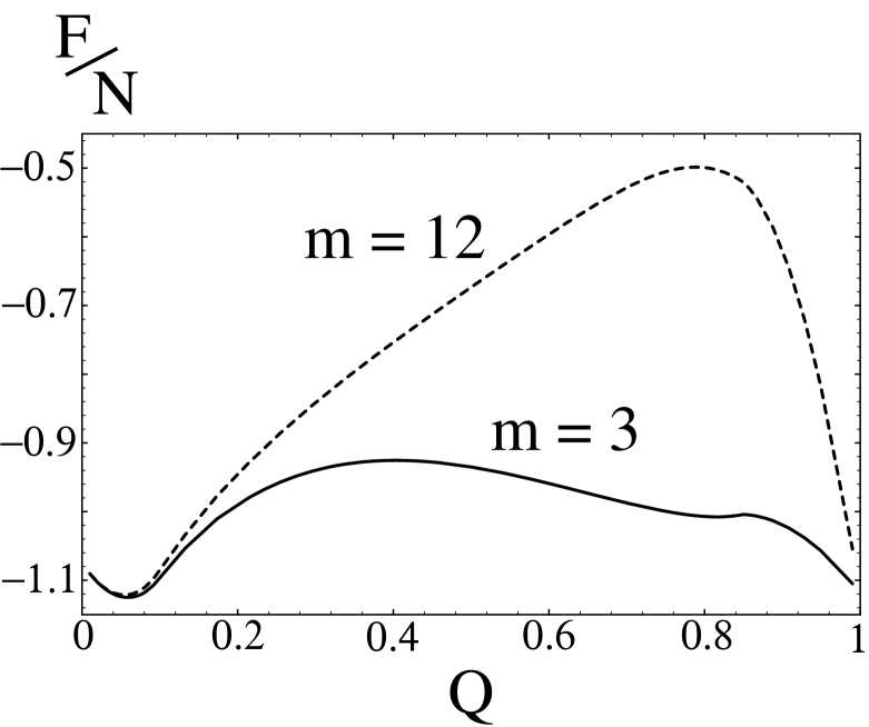
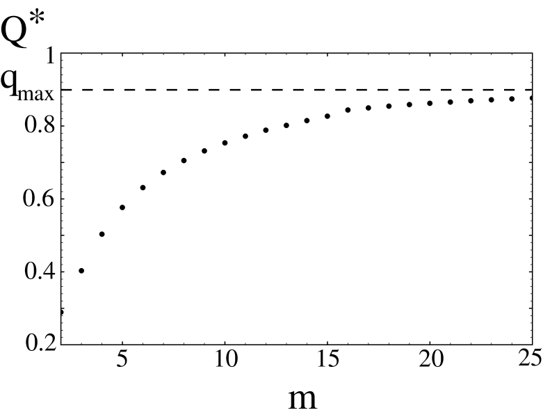
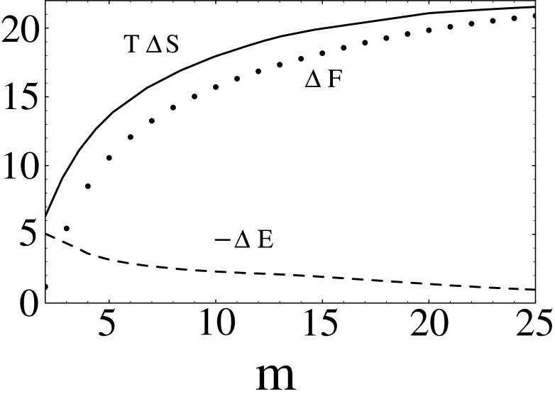
FIG. 1.:

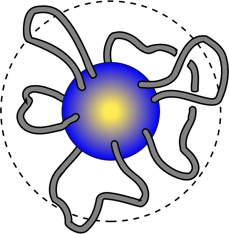
FIG. 2.:

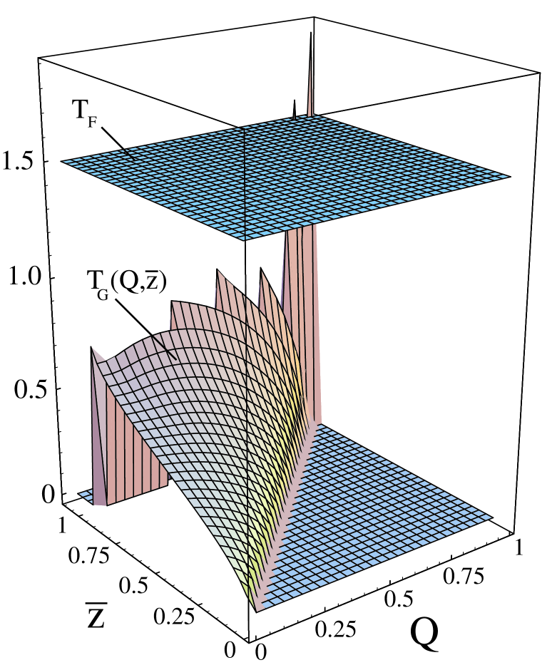
FIG. 3.:

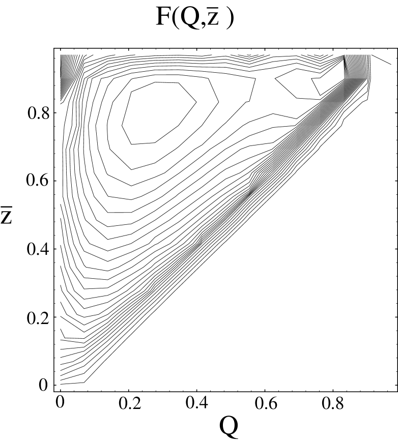
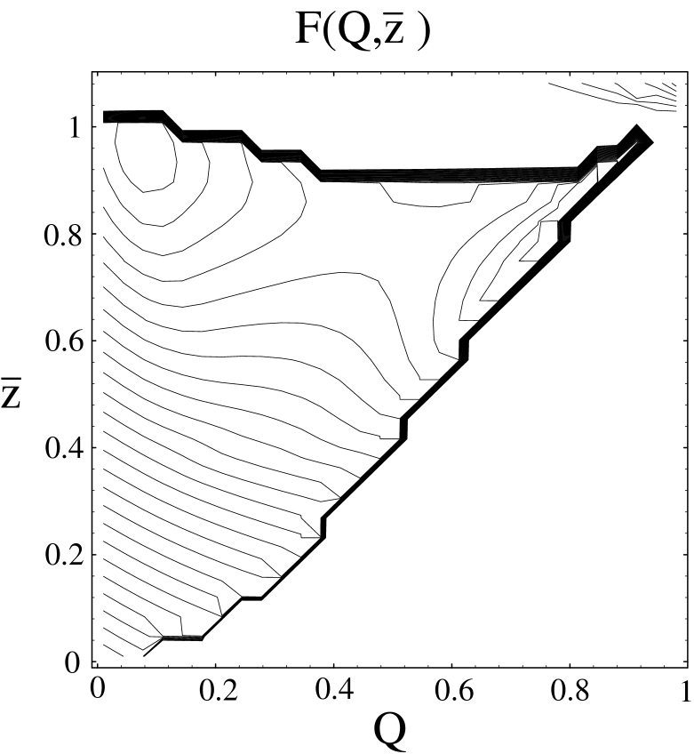
FIG. 4.:

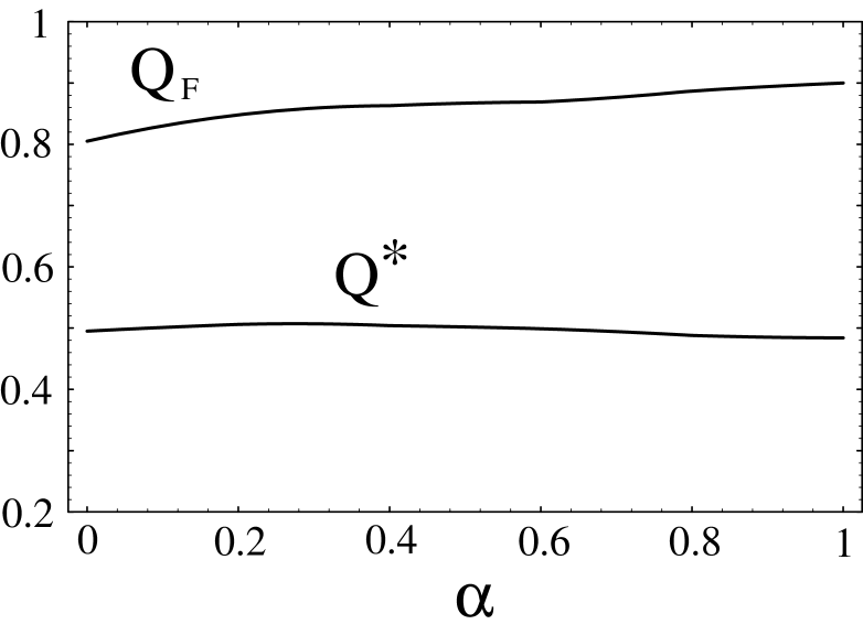
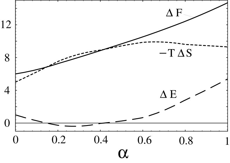
FIG. 5.:

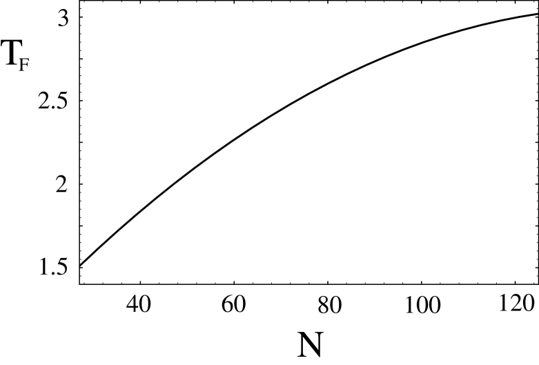
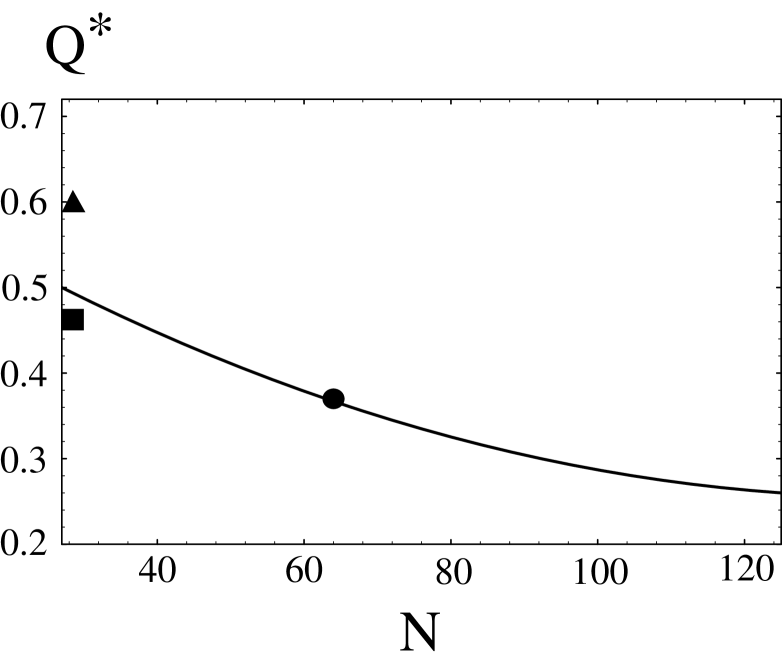
FIG. 6.:

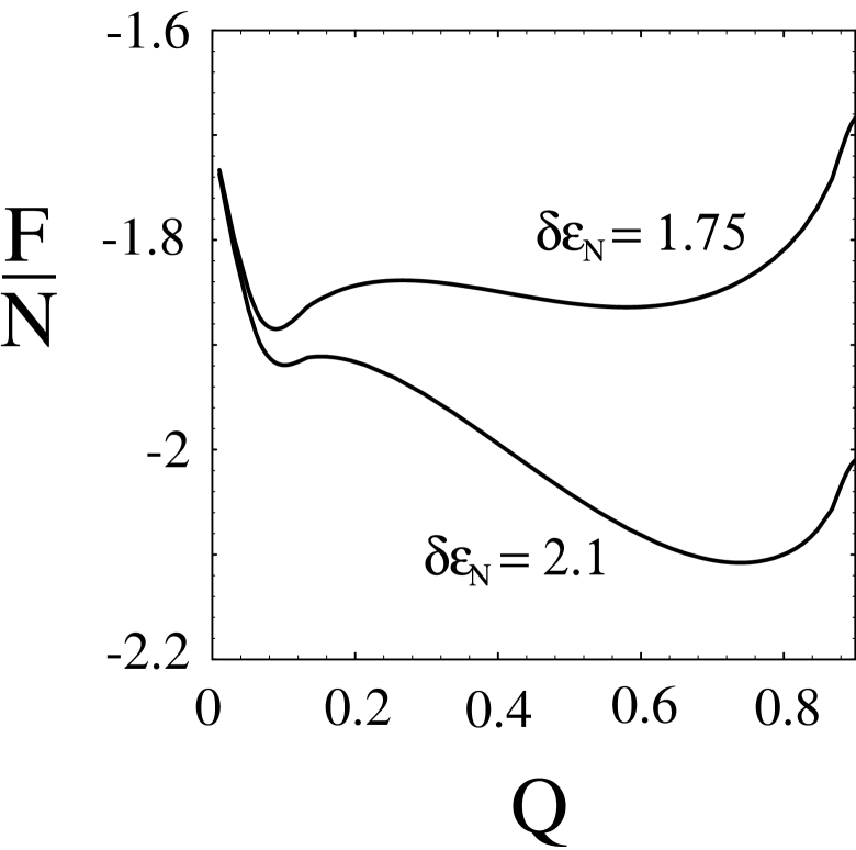
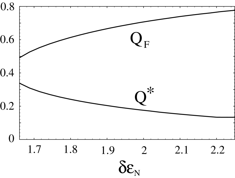
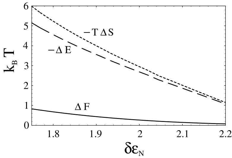
FIG. 7.:

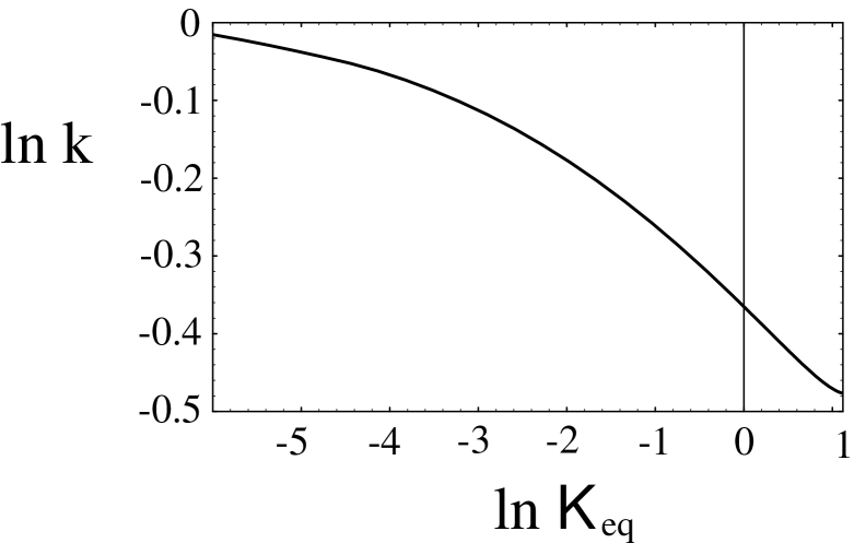
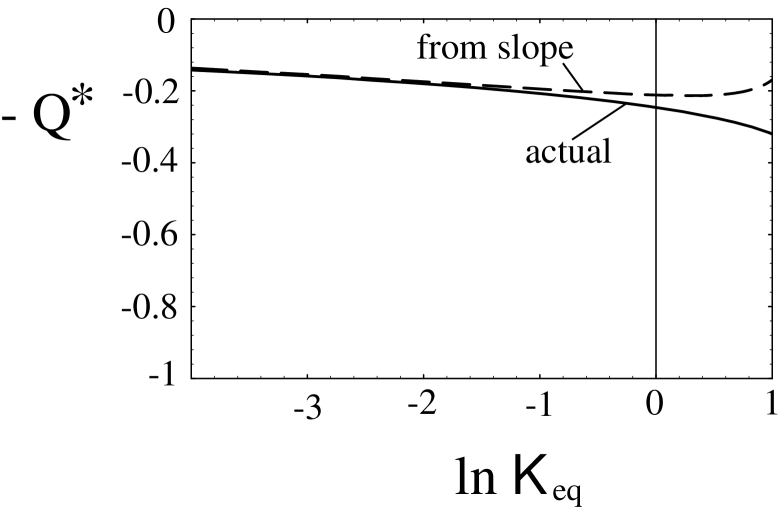
FIG. 8.:

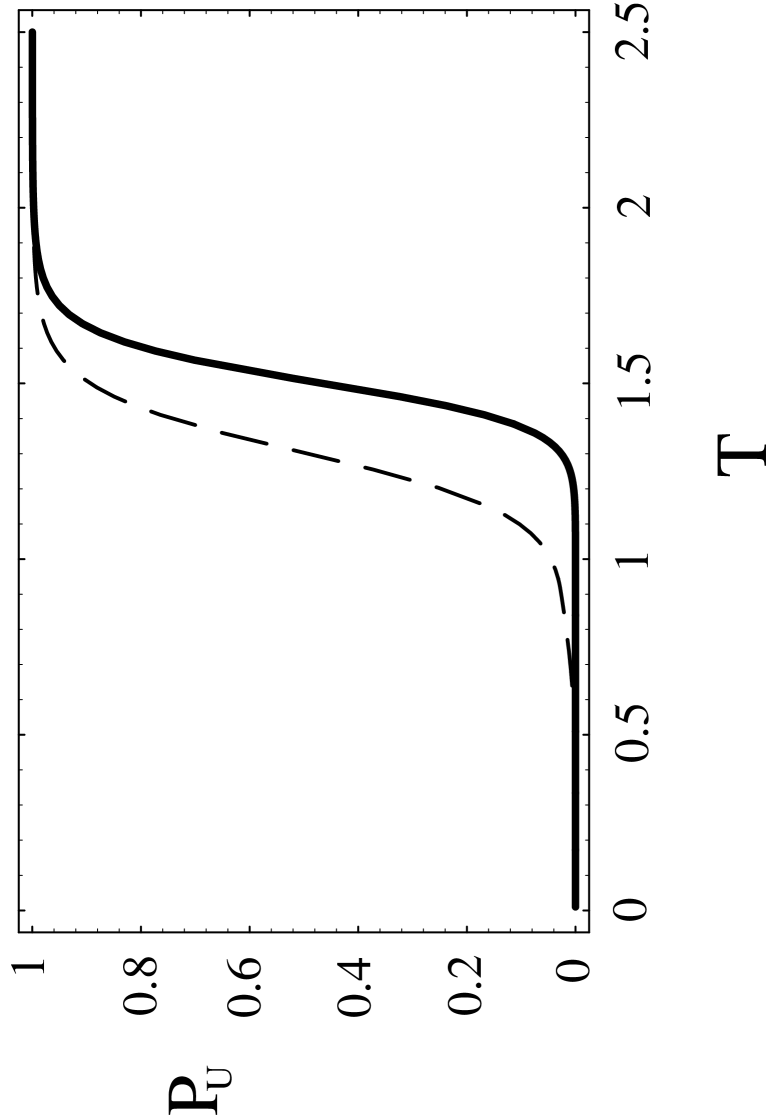
FIG. 9.:

REFERENCES

- [1] J. Bryngelson and P. G. Wolynes, (1987) P.N.A.S., 84, 7524-7528 .
- [2] J. Bryngelson, J.O. Onuchic, N.D. Socci, and P.G. Wolynes, (1995) PROTEINS: Structure,Function, and Genetics, 21, 167-195 .
-
[3]
M.S. Friedrichs and P.G. Wolynes (1989) Science
246, 371
D. Thirumalai and Z. Guo, Biopolymers 35 137 (1995) -
[4]
A. Kolinski, A. Godzik, and J. Skolnick, (1993)
J. Chem. Phys. 98 (9), 7420
N.D. Socci and J.N. Onuchic, (1994) J. Chem. Phys, 101, 1519-1528.
K.A. Dill, S. Bromberg, K. Yue, K.M. Fiebig, D.P. Yee, P.D. Thomas, and H. S. Chan (1995), Protein Science, 4, 561-602.
A. Sali, E. Shakhnovich, and M. Karplus, J. Mol. Biol. 235, 1614 (1994). - [5] J.N. Onuchic, P.G. Wolynes, Z. Luthey-Schulten, and N.D. Socci, Proc. Natl. Acad. Sci. USA, 92, 3626-3630 (1995)
-
[6]
M. Mezard, G. Parisi, and M.A. Virasoro, “Spin Glass
Theory and Beyond”, Singapore: World Scientific, 1986.
K.H. Fischer and J.A. Hertz, “Spin Glasses”, Cambridge: Cambridge Uneversity Press, 1991. -
[7]
L.D. Landau, E.M. Lifshitz , “Statistical Physics, Part 1”,3rd ed.
J.B.Sykes, M.J. Kearsley trans., Course of Theoretical Phyusics, Vol. 5.
Oxford:Pergamon Press, 1980.
N. Goldenfeld, “Lectures on Phase Transitions and the Renormalization Group”,Addison-Wesley, 1992. -
[8]
T. Garel and H. Orland (1988) Europhys. Lett., 6, 307.
E.I. Shakhnovich and A.M. Gutin (1989) Europhys. Lett., 8, 327.
E.I. Shakhnovich and A.M. Gutin (1989), Biophysical Chemistry, 34, 187. - [9] M. Sasai and P.G. Wolynes, Phys. Rev. Lett. 65, 2740 (1990).
- [10] B. Derrida ,(1981) Phys. Rev. B, 24, 2613 .
-
[11]
Z. Luthey-Schulten,B.E. Ramirez, and P.G.Wolynes, (1995)
J. Phys. Chem., 99, 2177-2185 .
J. G. Saven and P.G. Wolynes J. Mol. Biol. 257, 199 ,(1996). - [12] S.S. Plotkin, J. Wang, P.G. Wolynes, Phys. Rev. E, to appear
- [13] B. Derrida and E. Gardner, (1986) J. Phys C, 19, 2253 - 2274 .
-
[14]
M.S. Friedrichs and P.G. Wolynes (1989) Science
246, 371.
M.S. Friedrichs, R.A. Goldstein and P.G. Wolynes, J. Mol. Biol. 222 1013 (1991). -
[15]
S. Ramanathan and E. Shakhnovich, Phys. Rev. E,
50, (2) p. 1303 (1994).
V.S. Pande, A.Y. Grosberg, and T. Tanaka, J. Phys. II France, 4, (1994) 1771-1784. - [16] P.J. Flory ,(1956) J. of Am. Chem. Soc., 78, 5222 .
- [17] G.S. Huang and T. G. Oas, Proc. Natl. Acad. Sci. USA 92 6878 (1995)
- [18] S.E. Jackson and A.R. Fersht Biochemistry 30, 10428 (1991).
- [19] J.F. Douglas and T. Ishinabe ,(1995) Phys. Rev. E, 51, 1791 .
- [20] Unless otherwise indicated, all entropies have dimensions of Boltzmann’s constant .
- [21] Unless otherwise indicated, all temperatures have units of energy, with Boltzmann’s constant included in the definition of .
- [22] R. A. Goldstein, Z. A. Luthey-Schulten, and Peter G. Wolynes (1992) Proc. Natl. Acad. Sci. USA, 89, 4918
- [23] B. Derrida and G. Toulouse, (1985) J. Physique Lett., 46, 223-228.
- [24] N.D. Socci and J.N. Onuchic, private communication.
- [25] T. Pascher, J.P. Chesick, J.R. Winkler, and H.B. Gray, Science, 271, 1558 (1996).
- [26] N.D. Socci and J. N. Onuchic J. Chem. Phys., 101, (2) (1994).
- [27] L.S. Itzhaki, D.E. Otzen, and A.R. Fersht J. Mol. Biol. 254, 260 (1995).
- [28] E.M. Boczko and C.L. Brooks, Science 269 393 (1995)
- [29] J.N. Onuchic, N.D. Socci, Z. Luthey-Schulten, and P.G. Wolynes, Science to appear.