Earthquake statistics and fractal faults

Abstract

We introduce a Self-affine Asperity Model (SAM) for the seismicity that mimics the fault friction by means of two fractional Brownian profiles (fBm) that slide one over the other. An earthquake occurs when there is an overlap of the two profiles representing the two fault faces and its energy is assumed proportional to the overlap surface.

The SAM exhibits the Gutenberg-Richter law with an exponent $\beta$ related to the roughness index of the profiles. Apart from being analytically treatable, the model exhibits a non-trivial clustering in the spatio-temporal distribution of epicenters that strongly resembles the experimentally observed one. A generalized and more realistic version of the model exhibits the Omori scaling for the distribution of the aftershocks.

The SAM lies in a different perspective with respect to usual models for seismicity. In this case, in fact, the critical behaviour is not Self-Organized but stems from the fractal geometry of the faults, which, on its turn, is supposed to arise as a consequence of geological processes on very long time scales with respect to the seismic dynamics. The explicit introduction of the fault geometry, as an active element of this complex phenomenology, represents the real novelty of our approach.

¹Dipartimento di Fisica, Università dell’Aquila

Via Vetoio I-67100 Coppito, L’Aquila, Italy

² Centro Ricerche ENEA, Località Granatello

C.P. 32 - 80055 Portici (Napoli) Italy

³Dipartimento di Fisica, Università di Roma ’La Sapienza’

P.le A.Moro 2 I-00185 Roma, Italy

⁴ Dipartimento di Fisica, Università di Como

Como, Italy

PACS NUMBERS: 91.39.Px, 05.45.+j

1 Introduction

Recently, theoretical models have acquired an increasing relevance in the study of the seismicity. Their aim is to fill up the gap between the experimental knowledge and the theoretical comprehension of the phenomenon.

One of the most serious problem which geologists have to face is the lack of complete catalogues extended over long time periods. This makes difficult to improve the general comprehension about earthquakes. By studying theoretical models, one then tries to focus on some particular ingredients, which are supposed to be essentials, and then tries to understand as much as possible of the seismic behaviour. In this way one can compare the specific predictions of the models with those obtained from the real catalogues.

Though the dynamics of earthquakes is very complex there are some simple basic components which have to be taken into account in a model:

• earthquakes are generated by a very slow discontinuous driving of a fault;

• the occurrence of earthquakes is intermittent, i.e. they occur as abrupt rupture events when the fault can no longer sustain the stress;

• there are two separate time scales involved in the process; one is related to the stress accumulation while the other, which is orders of magnitude smaller, is associated to the duration of the abrupt releases of stress.

Many forms of scaling invariance appear in seismic phenomena. The most impressive feature is the celebrated Gutenberg-Richter law [1] for the magnitude distribution of earthquakes. It states that the probability $P(E)dE$ that an earthquake releases an energy in the interval $\left[E,E+dE\right]$ scales according to a power-law

$$P(E)\sim E^{-\beta-1}$$ (1)

with an exponent $\beta$ of order of unity whose eventual universality represents matter of debate.

The Omori law [2] for the time correlations of aftershocks (i.e. seismic events which happen as a consequence of a main earthquake) is another example of scaling behaviour in the seismic phenomenology and one of the most difficult to reproduce in simplified models.

In the last decades there has been an increasing evidence for the space-time clustering [3] of the earthquake epicenters. In particular there are experimental evidences suggesting that the epicenter distributions is self-similar both in space and in time.

Unfortunately, the complexity of modelling the motion of a fault system, even in rather well controlled situations such as the San Andreas fault in California, is a highly difficult task and it is still controversial what is the correct theoretical framework at the very origin of scaling laws. It is thus important to individuate models as simple as possible that are able to exhibit the main qualitative features of the fault dynamics. Their physical relevance stems from the specific predictions on the real seismic activity which might be verified from experimental data.

One of the first attempt in this direction is due to Burridge and Knopoff [4] who introduced a stick-slip model of coupled oscillators to mimic the interaction of two fault surfaces. In practice, one considers blocks on a rough support connected to one another by springs. They are also connected by other springs to a driver which moves at a very low constant speed. The blocks stick until the spring forces overwhelms the static friction and then one or more blocks slide, releasing an ‘earthquake’ energy proportional to the sum of the displacements. In the frame of the inferior plate, if $x_{i}$ denotes the position of th $i$-th block, the equations of motion are

$$m_{i}\ddot{x_{i}}=k_{c,i}(x_{i+1}-x_{i})-k_{c,i-1}(x_{i}-x_{i-1})-k_{p,i}(x_{i}-vt)+F_{i}(\dot{x_{i}})$$ (2)

where $F_{i}(\dot{x_{i}})$ represents the friction force which depends on the block velocity $\dot{x_{i}}$. In the original model the friction force, zero for zero velocity, increases progressively as the velocity increases up to a certain maximum value. This model exhibits the Gutenberg-Richter law for the distribution of the energy released during an earthquake and it allows for the presence of aftershocks. Up to now the original model of Burridge and Knopoff remains the only one able to explain the presence of aftershocks without ad hoc modifications.

A numerical integration of the Newton equations for a one-dimensional chain with a large number of homogeneous blocks has been performed by Carlson and Langer [5]. Their model differs from that of Burridge and Knopoff in the form of the friction force which is supposed to be identical for all the blocks, neglecting the inhomogeneities of the crust. It has been shown that the model exhibits the Gutenberg-Richter law [1] (see also [6] for the connection with the chaotic behaviour of the system).

More recently it has been suggested that the qualitative aspects of earthquakes (and of Burridge and Knopoff models) could be captured by the so-called Sandpile models, which are the paradigm of a large class of models showing Self-Organized Critical (SOC) [7]. The concept of Self-Organized Criticality (SOC) has been invoked by Bak, Tang and Wiesenfeld [7] to describe the tendency of dynamically driven systems to evolve spontaneously towards a critical stationary state with no characteristic time or length scale. An example of this behaviour is provided by Sandpile models: sand is added grain by grain in a pile on a $d$-dimensional lattice until unstable sand (too large local slope of the pile) slides off. In this way the pile reaches a steady state where additional sand grains fall off the pile by avalanche events. This steady state is critical since avalanches of any size are observed. According to this picture of Self-Organized Criticality, during its whole evolution the earth would have reached a marginally stable state in which any small perturbation could give rise to relaxation processes, earthquakes in this case, that can be small or cover the entire system. In this way the earthquakes would be the equivalent of avalanches for Sandpiles models. The main ingredient in this picture would be the interplay between the slow dynamics, represented by the stress accumulation, and the fast dynamics of earthquakes. The latter would modify the earth crust which, on its turn, can give rise to earthquakes and so on, with a feedback mechanism that would be at the origin of the self-organization.

There exists a whole generation of SOC models proposed to explain the scale-invariant properties of earthquakes [9, 10]. These type of models suggest however that there is no stress accumulation before a big earthquake and the exponent of the Gutenberg-Richter law is expected (with the exception [8] that we mention hereafter) to be universal. In addition the space-time distribution of the epicenters has no clear relation with the experiments where non-trivial clustering are present.

It is worth to recall in this framework the model proposed by Olami, Feder and Christensen [8]. Their model maps the two dimensional version of the Burridge-Knopoff spring-block model in a cellular automaton and it gives a good prediction of the Gutenberg-Richter law with a non-universal value of the $\beta$-exponent, which varies with the level of non-conservation of the model and could account for the $\beta$ variances observed in nature.

In order to go beyond the limitations of these models, we have recently proposed an alternative approach [11] where the critical behaviour is not self-organized but stems from the fractal geometry of the faults [12, 13, 14]. In this perspective the faults are supposed to be formed as a consequence of geological processes on very long time scales with respect to the seismic dynamics. Looking at the system on the time scale of human records the fault structure can be considered assigned and just slightly modified by earthquakes.

In particular, we have introduced the so-called Self-affine Asperity Model (SAM) [11] which mimics the fault dynamics by means of the slipping of two rough and rigid brownian profiles one over the other. In this scheme an earthquake occurs when there is an intersection between the two profiles. The energy released is proportional to the overlap interval. This model, apart from being analytically treatable, exhibits some specific features which follow from the fractal geometry of the fault. In particular it reproduces the Gutenberg-Richter law with an exponent $\beta$ which is non-universal since it depends on the roughness of the fault profiles. It predicts the presence of a local stress accumulation before a large seismic event. Moreover it allows one to analyze and investigate the complex phenomenology of the space-time clustering of epicenters. The model exhibits, in fact, a long-range correlation of the events which corresponds to a self-similar distribution of the spatial and temporal epicenter sets. In this scheme it is also possible to include the analysis of the origin of aftershocks and show that, in a natural generalization of the model, they follow the celebrated Omori’s law.

In this paper we describe in detail the SAM. The analytical results are, step by step, tested numerically and, whenever possible via the comparison with experimental data.

The outline of the paper is the following. In sect. II we introduce the model and we recall some properties of fractional Brownian profiles. Sect. III is devoted to the discussion of the Gutenberg-Richter law. We show that the SAM follows this scaling with an exponent $\beta$ that we relate analytically to the roughness of the brownian profile. This allows us to draw some conclusions on the non-universality of the exponent $\beta$. In sect. IV we discuss the problem of the distribution of epicenters both from the spatial point of view and the temporal one. The SAM exhibits a non-trivial clustering of epicenters which reproduces the experimental results and can be analytically explained by exploiting the properties of the fractional Brownian profiles. The problem of the power spectrum of the temporal sequence of earthquakes is also discussed. Sect. V is dedicated to the introduction of a more realistic version of the SAM model. This version, which takes into account the local rearrangement of the earth crust as a consequence of the earthquakes, exhibits a non-trivial scaling in the distribution of the aftershocks, according the Omori’s law. Finally in sect. VI we draw the conclusions. The paper is completed by two appendices on the statistics of the fractional Brownian profiles.

2 The model

Many authors pointed out that natural rock surfaces can be represented by fractional brownian surfaces over a wide scale range [12, 13] and that also the topographic traces of the fault surfaces exhibit scale invariance [17]. A fault can thus be regarded as a statistically self-affine profile $F_{H}(t)$, whose height scales as $|F_{H}(t+\tau)-F_{H}(t)|\sim\tau^{H}$. In $d=2$, such a profile $F_{H}(t)$ can be generated by fractional Brownian motion (fBm) with exponent $H$, the Hurst exponent, and in $d=3$ by the standard generalization given by brownian reliefs [18, 19]. The exponent $0\leq H\leq 1$ controls the roughness of the fault where the standard brownian profile corresponds to $H=1/2$, and a differentiable curve corresponds to $H=1$. Just to give an example let us recall how it is possible to generate a brownian profile. In the one-dimensional case one can generate $L$ random variables (r.v.) $\{X_{1},...,X_{L}\}$ according to the following algorithm:

$$X_{i}=\left\{\begin{array}[]{ll}1&\mbox{with prob. $p=1/3$}\\ 0&\mbox{with prob. $p=1/3$}\\ -1&\mbox{with prob. $p=1/3$}\end{array}\right.$$

On a one-dimensional lattice of $L$ sites one can thus define a stochastic function

$$S(n)=S_{0}+\sum_{i=1}^{n}X_{i}\,\,\,\forall n\leq L$$ (3)

where $S_{0}$ is an arbitrary integer number. The (3) defines, in the limit $n\rightarrow\infty$ a self-affine profile of fractal dimension $D=1.5$. More in general the fractal dimension of the profile is well known to be $D_{F}=d-H$. For further details we refer to the appendix A.

The explicit introduction of the fault geometry in a model for seismicity was already been supposed by Huang and Turcotte [12]. They introduced a static model where the average of all the seismic events contributing to the Gutenberg-Richter law is taken over many uncorrelated realizations of one single fractal profile. The purpose of this letter is to introduce a dynamical model, called Self-affine Asperity Model (SAM), that describes the seismic activity considering two profiles sliding one over the other instead of only one as in [12]. Such a model has the advantage to exhibit strong spatial and temporal correlations also between far away seismic events, and allows us to infer some specific and new predictions about the relation between the roughness of the fault $H$ and the scaling exponent of the Gutenberg-Richter law as well as on the spatio-temporal distribution of epicenters.

Note how this model represents an alternative approach with respect to the SOC models. In this case, in fact, one supposes as lacking the interplay between the fault structure and the seismic events. The latter is supposed not to modify substantially the fault geometry. In this sense one is in a sort of limit of infinite rigidity of the Burridge-Knopoff models.

Operatively, the SAM is defined by the following dynamical rules:

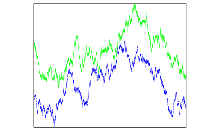
Figure 1: Fault planes realized by two Brownian profiles put in contact in one point.

(i) We consider two profiles, say $S^{\prime}(n)$ and $S^{\prime\prime}(n)$, with $n=1,...,L$, on parallel supports of length $L$ at infinite distance. The initial condition is obtained by putting them in contact in the point where the height difference is minimal so that (see Fig.1)

$$\left\{\begin{array}[]{l}S^{\prime}(n)=S^{\prime\prime}(n)+max_{j\in\{1,...,L\}}\{S^{\prime}(j)-S^{\prime\prime}(j)\}\\ n=1,...,L\end{array}\right.$$

(ii) The successive evolution is obtained by drifting a profile in a parallel way with respect to the other one, at a constant speed $v$, so that $S^{\prime}(n;t)=S^{\prime}(n-v\,t)$;

(iii) At each time step $t$, one controls whether there are new contact points between the profiles, i.e. whether $S^{\prime}(n;t)-S^{\prime\prime}(n)<0$ for some $x$ value. An intersection represents a single seismic event and starts with the collision of two asperities of the profiles. The energy released is assumed to be proportional to the breaking area of the asperities, i.e. the extension of the hypersurfaces, in general of dimension $(d-1)$, involved in the collision of the asperities during an earthquake. In the case $d=2$ the energy released is given by the sum of the lengths of the two segments indicated with $A$ and $B$ in Fig.1;

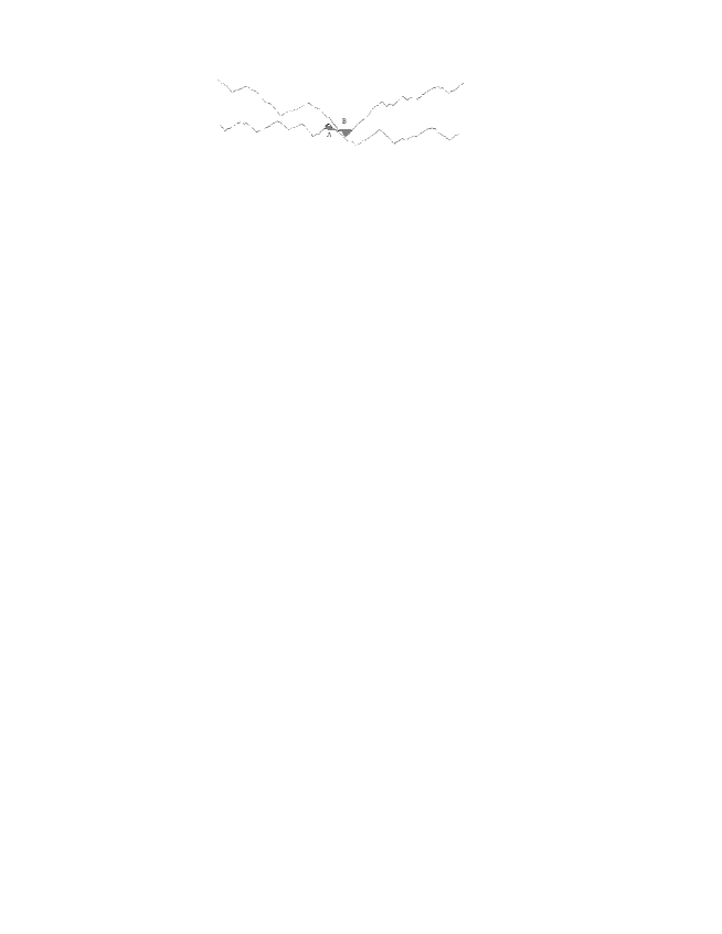
Figure 2: Sketch for the definition of the energy released during an earthquake. It is assumed proportional to the breaking area (the $(d-1)$-dimensional sets $A$ and $B$) between the two asperities: $E\propto A+B$.

(iv) We do not allow the developing of new earthquakes in a region where a seismic event is already taking place, i.e., with reference to the Fig.2, we do not take into account the earthquakes which eventually take place in the region $A$ and $B$ of the two profiles, until $A$ and $B$ have a non-zero overlap.

Rule III is a consequence of the proportionality between the energy released during an earthquake and its seismic momentum $M_{0}$, which, on its turn, is proportional to the average displacement of a fault during an earthquake. It is obviously possible to consider more sophisticated schemes and the work along these lines is already in progress.

With these rules, the motion of the two profiles simulate the slipping of the two walls of a single fault. The points of collision are the points of the fault where the morphology prevents the free slip: these are the points where there is an accumulation of stress and, consequently, a raise of pressure. When the local pressure exceeds a certain threshold, it happens a breaking, an earthquake, which allows to relax the stress and redistribute the energy, previously accumulated, all around. We assumed that the region between the two sliding profiles of the fault is empty or filled by a granular medium, coherently to the observation that the fault gauge is a zone of fractured rocks. According to the paper by Herrmann et al. [20] one could think to this granular medium as composed by roller bearings between the two surfaces. The existence of large region between the two rough surfaces could then be related to the so-called seismic gap, namely an extended area two tectonic plates can creep on each other without producing either earthquakes or the amount of heat expected from usual friction forces. This zone slides and has no influences on the dynamics due to its relatively lower viscosity.

For sake of simplicity, in this version of the SAM, there is no real breaking of the profiles as a consequence of an earthquake and the profiles maintain their structures after a crash. Thus are in the opposite perspective than SOC models. Since the earthquake dynamics has no effect on the structure of the profile. Realistic situations could well correspond to intermediate cases, of course.

It is possible to introduce a more realistic breaking mechanism where there is also a modification of the asperity form after an earthquake. We will discuss this possibility in sect.V and we will show there how it is possible, in this framework, to reproduce the Omori’s law.

It is worth to stress that the SAM exhibits a strong non-locality since a collision in a point $x$, at the time $t$ can trigger, at later time, a subsequent event also very far away. One of the main advantage of the SAM consists in the possibility of deriving various analytic results using the properties of brownian profiles.

3 The Gutenberg-Richter law and the non-universality of the $\beta$-exponent

In 1956, Gutenberg and Richter [1] noticed the dependance of earthquakes frequency from their magnitude: the greater the magnitude, the smaller the frequency. The relation between the frequency and the magnitude of earthquakes is:

$$\log_{10}{N(M>m)}=a-bm,$$ (4)

where $N(M>m)$ is the number of earthquake with a magnitude greater than $m$ while $a$ and $b$ are two empirical parameters. The $b$ value is generally in the range $0.8<b<1.4$ depending on the earth region considered and the stress level of the region itself.

Relation (4) is the most important statistical representation of seismicity and the understanding of the underlying mechanisms is of fundamental importance for the comprehension of earthquakes and their prevision. Several studies have been achieved to understand the origin of the universality of the Gutenberg-Richter relation but, despite the simplicity of this relation, there is no understanding of the underlying mechanisms. The $b$ value might depend on three factor: (1) the geometrical properties of the fault, (2) the physical properties of the medium and (3) the stress level of the seismic region. In this section we show that, in the framework of the SAM, the $b$ value is essentially determined by the fault geometry and in particular by its fractal dimension. The magnitude $M$ is not the only indicator of the earthquakes strength; another quantity used to describe the earthquake intensity is the seismic moment defined by the relation:

$$M_{0}=\int_{A}\mu SdA,$$ (5)

where $\mu$ is the rigidity modulus of the medium under consideration, $S$ is the slip and $A$ is rupture area. From dimensional analysis it is obvious that the energy $E$ released by an earthquake is proportional to its moment. There is an empirical relation between the seismic moment (or energy) and the magnitude:

$$\log_{10}{E}=cM+d,$$ (6)

where $E$ is the released energy. From eq. (4) and (6) we easily obtain the energy distribution for earthquakes:

$$P(E)\sim E^{-\beta-1},$$ (7)

where $P(E)$ is the probability of an earthquake releasing an energy $E$ and $\beta=b/c$.

In order to describe the seismic phenomenology a model for the fault slip has to verify equation (7): we thus will study the energy distribution for the model defined in the previous section (SAM).

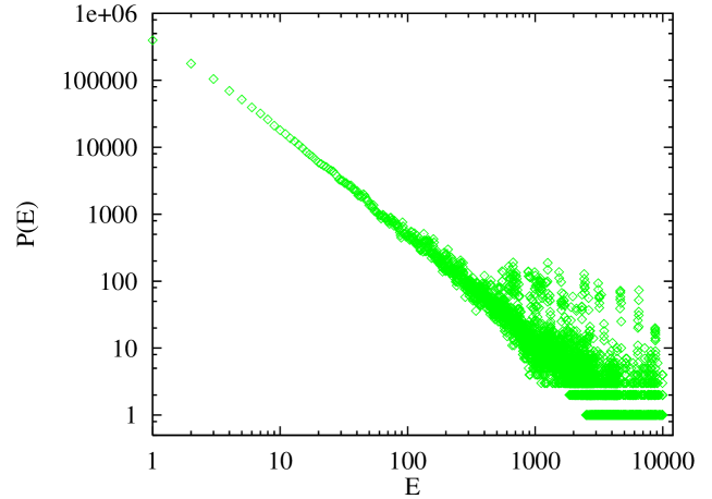
Figure 3: Probability density of the earthquakes releasing an energy $E$ vs. $E$ for roughness index $H=1/2$.

The numerical simulations provide a clear evidence that our model exhibits the Gutenberg-Richter law (7), see Fig.3. As we have defined in the previous section, the energy released during an earthquake is essentially given by the length of the superposition between the fluctuations of the two self-affine profiles. Remembering that the difference between two self-affine profiles is a self-affine profile itself, we can consider only the profile given by the difference between the upper profile and the lower profile: the energy distribution will be simply the length distribution of the segment obtained intersecting the difference profile with a straight line.

If we consider a fractal ensemble having a dimension $D=d-H$ embedded in a $d$-dimensional Euclidean space, the intersection between the ensemble and an hyperplane of dimension $d-1$ will be an ensemble of dimension [17]:

$$D=(d-H)+(d-1)-d=d-H-1.$$

Therefore, the average extension of the hyper-areas given by the intersection between a self affine hyper-surface and an hyper-plane will be:

$$<a>_{L}\sim A^{\frac{H}{d-1}},$$ (8)

where the subscript $L$ indicates that we are considering a portion af hyperplane of extension $A\sim L^{d-1}$. In virtue of the self-affine nature of the considered ensemble, the hyper-areas distribution will be:

$$d(a)\sim a^{-\beta-1}.$$

From the last equation we can compute the mean extension of the hyperareas:

$$<a>_{L}\sim\int^{L^{d-1}}_{0}a^{-\beta}da\sim L^{(d-1)(1-\beta)}$$ (9)

By comparing (8) and (9), one gets the relation between the exponent $\beta$ of the Gutenberg-Richter law in $d$ dimensions and the Hurst exponent which accounts for the fractal properties of the faults:

$$\beta=1-\frac{H}{d-1}.$$ (10)

In the three-dimensional case one has:

$$\beta=2-\frac{H}{2},$$ (11)

with $\beta\in[\frac{1}{2},1]$.

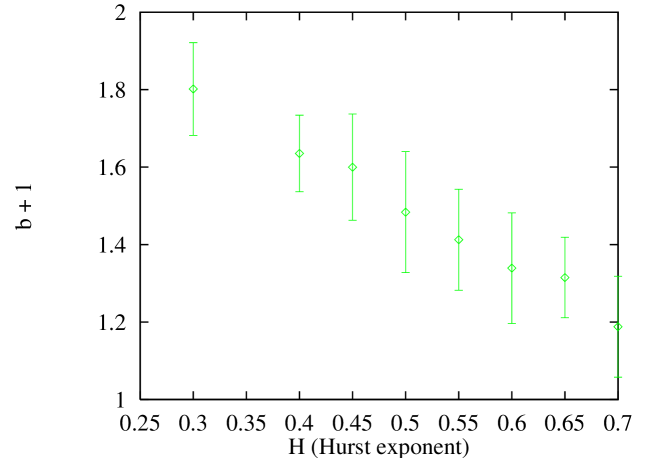
Figure 4: Exponent $\beta+1$ vs. the Hurst exponent $H$ for the SAM in $d=2$.

In order to check the (10) we have performed a numerical experiment in $d=2$. Fig. 4 reports the results of the $\beta$-value, as a function of the Hurst exponent, which are in good agreement with the expected relation $\beta=2-H$. The dependence of $\beta$-value on the roughness of the faults could then account for the non-universality of the $\beta$-value which would reflect the variability of the fractal dimension of the fault profiles around the world. In this perspective one could also try to relate the $\beta$-value to the age of a given fault profile. By supposing that the effect of the fault slipping and of the earthquakes is a smoothing of the profiles, i.e. an increase of $H$, one could guess that the older the fault profile, the smaller the $\beta$-value.

4 Space-time distributions of epicenters

Let us now try to analyze the problem of the space-temporal clustering of the earthquakes epicenters. Many authors [3, 15, 16], pointed out that the epicenter tend to cover a fractal set with a fractal dimension which is a highly irregular function of space and time. One of the most interesting feature is represented by the evidence that the spatial distribution of the epicenters along a linear seismogenetic structure seems to exhibit self-similar properties. Results of the same kind have been reported for single ”transform” faults. This could lead to the conclusion that the non-homogeneity of the spatial distribution of the epicenters is due to some peculiar phenomenon occurring also in a single linear fault and just partly to the fractal distribution of the faults.

Similar properties are exhibited by the temporal distribution of events whit a non-homogenous structure, made of periods of quiescence and bursts of activity. Along the same region there could be sub-regions with non-homogeneous and also very different behaviours.

Thanks to the simple dynamics of the SAM model it is possible to study, whether analytically or numerically the complex space-time distribution of the epicenters. Operatively the space location of an epicenter is defined in correspondence of the first point of contact of the two colliding asperities belonging to the two profiles.

As far as spatial distribution of earthquakes is concerned, our simulations provide a good evidence of a spatial clustering of epicenters on a set with fractal dimension smaller than $1$. In particular we obtained a value of the fractal dimension $d_{ep}$ in the range $d_{ep}\simeq 0.8-0.9$ for $H$ varying in the interval [0.3,0.7] and for different lengths of the system between $L=1000$ and $L=50000$.

By numerical analysis of the model the values of $d_{ep}$ seem to decrease with increasing $H$ and seems to remain nearly constant with respect to variations of the system dimensions and of $H$. These results are not of immediate explanation; if the fault profiles could slip for an infinite time, in fact, each point of the inferior profile could be, theoretically, an epicenter because it, sooner or later, would be hit by an asperity of the superior fault profile. In this way we would have that $\lim_{t\rightarrow\infty}d_{ep}=\lim_{L\rightarrow\infty}d_{ep}=1$, and the set of epicenters thus becomes a compact set. This intuitive idea turns out to be correct since the observed non-integer fractal dimension is a non-trivial finite-size effect. It is possible to show analytically, for $H=0.5$, that the fractal dimension $d_{ep}(L)$ of the epicenter set in a fault of linear size $L$ is

$$d_{ep}(L)\simeq 1-\frac{\gamma\ln\ln L}{\ln L}\,\,\mbox{for large $L$}.$$ (12)

We will sketch here the main lines of the proof referring the reader for further details to appendix A.

First of all it is worth to remind that, according to the definition of the SAM, in order to obtain an infinite evolution of the system we necessarily need two fault profiles with a length $L$, which tends to infinity. One has first to create the two profiles separately and then to put them in contact. This because the average distance between the two profiles tends to increase as $L\rightarrow\infty$.

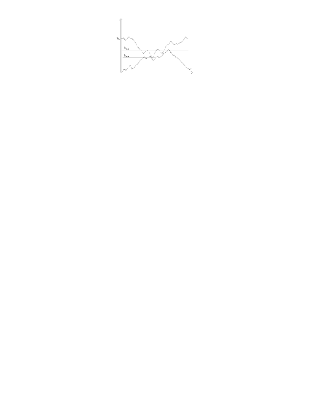
Figure 5: Scheme illustrating the region of heights $[h_{min},h_{max}]$ in which it is possible the occurrence of collisions between asperities. $h_{0}$ is a function of the length $L$ of the profiles and indicates their average distance.

In full generality, with reference to Fig.5, called $<S^{\prime}(n)>=S_{0}^{\prime}$, $<S^{\prime\prime}(n)>=S_{0}^{\prime\prime}$ and $h_{0}=max_{j\in\{1,...,L\}}\{S^{\prime}(j)-S^{\prime\prime}(j)\}$, one has, from eq.(2), $<S^{\prime\prime}(n)>=S_{0}^{\prime\prime}+h_{0}$ and putting, without loss of generality, $S_{0}^{\prime}=S_{0}^{\prime\prime}=0$,

$$<S^{\prime\prime}(n)-S^{\prime}(n)>=h_{0}.$$ (13)

The idea we want to use is that the number of epicenters $N_{E}$, for sufficiently large systems, will be proportional to the number of points of the inferior profile, $N(h,L)$, with an height $h$ between the minimum value, $h_{min}$, of the upper fault trace, and the maximum value, $h_{max}$, of the lower one, as shown in Fig.5:

$$N_{E}(L)\sim\int_{h_{min}(L)}^{h_{max}(L)}N(h,L)dh$$ (14)

where $N(h,L)$, for big values of $h$, can be written as

$$N(h,L)\sim\sqrt{L}\exp^{-\frac{3h^{2}}{4\eta L}}$$ (15)

where $3\eta/4$ is a constant dependent on the variance of the variables $\{x_{i}\}$ used to generate the profile. By inserting the (15) into the (14) one has

$$N_{E}(L)\sim\sqrt{L}\int_{h_{min}}^{h_{max}}\exp{-\frac{3h^{2}}{4\eta L}}.$$ (16)

Let us find an estimate of the $h_{min}$ and $h_{max}$ values in the limit $L\rightarrow\infty$ and consider the two faults to be brownian profiles ($H=1/2$) with length $L$.

In our case the variables $\{X_{i}\}$ $\{Y_{i}\}$ which compose the profiles are random variables with zero mean and variance $\sigma^{2}=2/3$. So the variables $\{\tilde{X_{i}}\}=\sqrt{3/2}\{X_{i}\}$ and $\{\tilde{Y_{i}}\}=\sqrt{3/2}\{Y_{i}\}$ will be random variables with zero mean and unitary variance. To these variables we can apply the so-called Iterated Logarithm Theorem (ILT) [21]. It states that, for a partial sum $S_{k}=\sum_{i=1}^{k}w_{i}$ of identically distributed random variables $\{w_{i}\}$ with $<w_{i}>=0$ and variance $\sigma^{2}\equiv<w_{i}^{2}>=1$, it holds:

$$P\Bigl{(}\lim_{k\rightarrow\infty}\sup\frac{S_{k}}{\sqrt{2k\ln\ln k}}=1\Bigr{)}=1$$ (17)

where $P(A=a)$ is the probability for the variable $A$ to have the value $a$. For the $H=\frac{1}{2}$ case we can also write $S_{inf}(k)=\sum_{i=1}^{k}X_{i}$ and $S_{sup}(k)=h_{0}+\sum_{i=1}^{k}Y_{i}$, where $\{X_{i}\}$ and $\{Y_{i}\}$ are uniformly distributed variables with zero mean, standard deviation $\sigma^{2}=2/3$ and $h_{0}=\max_{\forall i}(\sum_{k=1}^{i}X_{i}-Y_{i})$.

By using the ILT with profiles built with the normalized variables $\tilde{X}_{i}$ and $\tilde{Y}_{i}$ one obtains:

$$\begin{array}[]{l}\lim_{L\rightarrow\infty}\sup_{n\in\left[1,L\right]}\{S^{\prime}(n)\}=\frac{2}{\sqrt{3}}\sqrt{L\ln\ln L}\\ \lim_{L\rightarrow\infty}\inf_{n\in\left[1,L\right]}\{S^{\prime\prime}(n)\}=-\frac{2}{\sqrt{3}}\sqrt{L\ln\ln L}.\end{array}$$ (18)

One has also

$$\inf_{n\in\left[1,L\right]}\{S^{\prime}(n)\}=h_{0}+\inf_{n\in\left[1,L\right]}\{S^{\prime\prime}(n)\}$$ (19)

By defining the stochastic variables $\{Z_{i}=X_{i}-Y_{i}\}$ it will be, by definition,

$$h_{0}=\sup_{n\in\left[1,L\right]}\{\sum_{i=1}^{n}Z_{i}\}.$$ (20)

The variables $\{Z_{i}\}$ have zero mean and variance $\sigma^{2}=4/3$. So we can apply the ILT to the variables $\tilde{Z_{i}}=\frac{\sqrt{3}}{2}Z_{i}$ by getting

$$h_{0}=\frac{2\sqrt{2}}{\sqrt{3}}\sqrt{\ln\ln L}.$$ (21)

By comparing (18), (19) and (21) one easily gets the expression for $h_{min}$ and $h_{max}$:

$$\left\{\begin{array}[]{l}h_{min}=\frac{2}{\sqrt{3}}(\sqrt{2}-1)\sqrt{L\ln\ln L}\\ h_{max}=\frac{2}{\sqrt{3}}\sqrt{L\ln\ln L}\end{array}\right.$$ (22)

and, inserting these expressions in (16) and making a change of variables,

$$N_{E}(L)\sim L\int_{(\sqrt{2}-1)\sqrt{L\ln\ln L}}^{\sqrt{L\ln\ln L}}\exp^{-\frac{t^{2}}{2\eta}}dt=LI(L),$$ (23)

where $I(L)$ is an integral which tends to zero in the limit $L\rightarrow\infty$. We are interested to how this integral goes to zero.

The ”average theorem” for continuous function states that it will be possible to find a $\tilde{t}=\gamma(L)\cdot\sqrt{2\ln\ln L}$, with $\gamma(L)\in]\sqrt{2}-1,1[$, in such a way that

$$N_{E}(L)\sim L\cdot e^{-\frac{\tilde{t}^{2}}{2\eta}}\cdot\Delta t\sim\frac{L}{(\ln L)^{\tilde{\gamma}^{2}(L)/\eta}}$$ (24)

where $\Delta t$ is the integration interval and $\tilde{\gamma}(L)$ is the limit value of $\gamma(L)$ and we have neglected all the terms diverging slower than the logarithm.

Using the mass-length definition of fractal dimension,

$$d_{ep}=\lim_{L\rightarrow\infty}\ln N_{E}(L)/\ln L$$ (25)

, we obtain the relation

$$d_{ep}\simeq 1-\eta^{*}\frac{\ln\ln L}{\ln L}+O\Bigl{(}\frac{\ln\ln\ln L}{\ln L}\Bigr{)},$$ (26)

where $\eta^{*}$ is the mean value of $\tilde{\gamma}^{2}(L)/\eta(L)$. This implies that, according to what we had forewarned, $\lim_{L\rightarrow\infty}d_{ep}=1$, and, thus, that the fractal nature of the spatial distribution of epicenters is due to the faults finite size. The asymptotic value $d_{ep}=1$ is reached very slowly at increasing $L$ and it cannot be detected but by means of huge simulations. We have checked the validity of (26) for profiles with a linear size $L$ varying in the range $10^{2}-10^{6}$. Work is in progress to extend our results to the case of a generic roughness index $H$.

Let us now discuss the temporal correlations of earthquakes and in particular problem of the $1/f$ noise. A system is said to exhibit $1/f$ noise when its power spectrum scales as

$$S(f)\sim\frac{1}{f^{\alpha}},$$ (27)

with $\alpha$ smaller than 2. The interest on $1/f$ noise lies in its ubiquity in nature. $1/f$ noise has been detected in systems as divers as resistors, the hourglass, the flow of the rivers or of the cars in a traffic system. Despite much work has been devoted to this topic it is still lacking a general theory that explains the widespread occurrence of $1/f$ noise.

The fact that the power spectrum is connected to the autocorrelation function by the Wiener and Khintchin theorem leads some authors to the idea that the presence of the $1/f$ noise indicates the presence of self-similarity in the distribution of correlation times.

The autocorrelation function is usually defined as

$$C(t)=\frac{<E(t+t_{0})E(t_{0})>}{<E(t_{0})>^{2}}-1,$$ (28)

where $E(t)$ in our case represents the energy released by an earthquake occurred at the time $t$ and the averages are taken over the distribution of times $t_{0}$. If the energy presents a power-law distribution with an exponent greater than $-2$, as in our case, the average $<E(t)>$ will depend on its maximum value and then on the system dimension. We would have, in this way, a non consistent procedure to calculate the autocorrelation function. In order to overcome his difficulty one can use an alternative definition of the autocorrelation function which is independent of the scale of the system. If we define it as

$$C(t)=<E(t+t_{0})E(t_{0})>$$ (29)

it is possible to show [22] that the power spectrum $S(f)$ is linked to the Fourier transformation of $C(t)$, $<|E_{f}|^{2}>$, by the relation

$$<|E_{f}|^{2}>=S(f)+1/N$$ (30)

where $N$ represents the dimension of the system. We have also

$$S(f)=\sum_{f^{\prime}}<|E_{f^{\prime}}|^{2}>|W(f-f^{\prime})|^{2}.$$ (31)

where the function $W(f)$ takes into account the finite dimension of the system and tends to the delta function $\delta(0)$ for an infinite system. If $N$ is big enough one has:

$$S(f)\simeq<|E_{f}|^{2}>$$ (32)

and one can study the power spectrum simply analyzing the Fourier transform of the autocorrelation function (29).

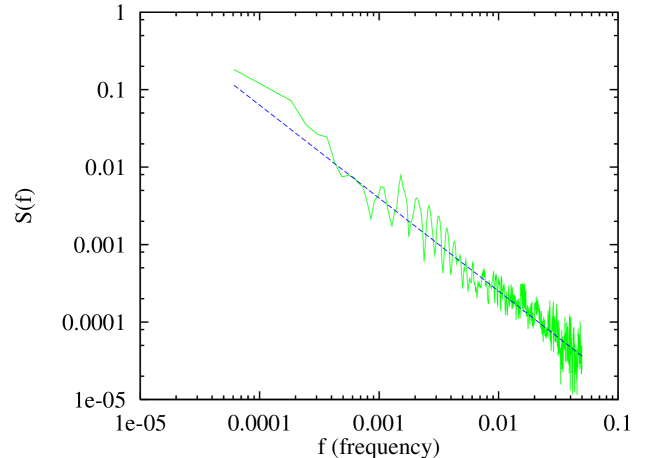
Figure 6: Power spectrum (solid line) for the temporal sequence of earthquakes in the SAM model. It shows a $1/f$ behaviour with an exponent $\alpha\simeq 1.2$ corresponding to the slope of the dashed line.

In our numerical simulation we have studied this function and the results, shown in Fig.6, gave

$$S(f)\sim f^{-\alpha}$$ (33)

with $\alpha\simeq 1.2$. This means that our model exhibits $1/f$ noise, i.e. it does not exist a maximum autocorrelation time and a seismic event may be influenced by another one very distant in time.

5 The Generalized SAM model

Up to now we have studied a version of the SAM model corresponding to the limit of infinite rigidity of the faults. The fault profiles are not modified by the seismic activity and one studies the statistics of earthquakes in the hypothesis that there is a complete time-scale separation between the seismic activity and the rearrangement of the earth crust. The latter would develop in very long times with respect to the scale of human records and this would justify the assumption.

We have shown how this model exhibits a good interpretation of the seismic phenomenology in a global sense: Gutenberg- Richter law, epicenter clustering. What is lacking is the description of what happens locally, i.e. as a consequence of a single event, both from the temporal point of view or from the spatial one. In particular it is not possible to obtain in such a scheme the Omori’s law for the distribution of aftershocks. These events are related to the situation in the neighborhood of the main shock epicenter after the occurrence of the main shock. They are ruled by the following empiric relation [2]

$$N(t)\sim\frac{1}{(t+c)^{\alpha}},$$ (34)

where $N(t)$ indicates the number of earthquakes occurred at the time $t$ after the main shock, $c$ is a constant and $\alpha$ is an exponent whose value ranges in the interval $[1.0\div 1.4]$. For enough long times $t$ one usually supposes $t>>c$ and the functional form of $N(t)$ is given by a pure power-law $N(t)\sim t^{-\alpha}$.

In this section we improve the model in order to include the rearrangement of the earth crust as a consequence of the occurrence of an earthquake. With this modification it is possible to describe the local phenomenology of seismicity and in particular to reproduce the Omori’s law.

The model is modified by considering the asperity breaking in the collisions. When two asperities collide a fracturing process starts in the smallest asperity (that one with the smallest section at the level of the epicenter). The fracture propagates inside the fault until it crosses again the fault profile. At this point the fracture stops and the resulting configuration represents the new fault profile in the region interested by the earthquake. The magnitude of the earthquake is assumed to be proportional to the linear extension of the fracture.

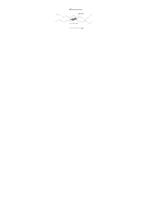
Figure 7: Scheme illustrating the mechanism for the breaking of the asperities in the generalized SAM model. When there is a collision between two asperities the weaker is broken. The shadowed region defines the broken area and the new profile after the collision.

In Fig.7 it is shown an example of fracturing process during an earthquake. The shadowed region is removed from the fault profile. The statistical properties of the fracture are supposed to be identical to the ones of the entire fault profile. This means that one has to consider a self-affine profile with the same Hurst exponent of the original fault.

In our simulations, we considered, for sake of simplicity, the case of a Brownian profile with $H=0.5$. Let us note that an earthquake in a certain point can trigger several other earthquakes, with smaller magnitude, which occur in the same region or in a very close region. In order to investigate the statistics of the aftershocks we identified all the aftershock occurring after a certain mainshock in the rupture region. A mainshock is defined as an earthquake above of a certain magnitude (in our simulations an earthquakes involving at least $100$ sites). Starting from this event one counts, as a function of the time elapsed from the mainshock, the number of earthquakes, with a magnitude smaller than that of the mainshock, occurring in the same region. One stops the counting when an earthquake with a magnitude greater or equal to the mainshock occurs.

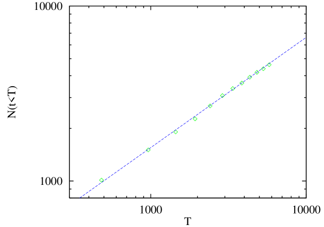
Figure 8: Cumulative distribution for the aftershocks: $N(t<T)$ is the number of aftershocks, events causally connected to the mainshock, occurred up to the time $T$, elapsed from the mainshock time.

We have studied the behaviour of the cumulative distribution of aftershocks, i.e. the number $N_{cum}(t<T)$ of earthquakes occurring before $T$ time steps after the mainshock. By averaging over many realizations (of the order of $10^{2}$) we have obtained the curve reported in Fig.8 that exhibits the Omori scaling law (34). For values of $t$ large enough one has the power law:

$$N_{cum}(t<T)\sim T^{1-\alpha}.$$ (35)

with the exponent $\alpha\simeq 0.37$. The numerical value of the exponent $\alpha$ is not in good agreement with real values. However, we have just considered the case of a one- dimensional profile embedded in a two-dimensional space and the model considers only one isolated faults, thus neglecting the effects of interaction among different faults. It would be interesting to study what happens considering the case of a two-dimensional surface too.

This generalized SAM recalls the work of Herrmann et al. [20] about the space-filling bearing. The analogy lies in the fact that one could think the interspace between the two fault planes as filled by a granular medium which is also composed by the broken asperities of the fault. The link is made closer by the fact that in our case the distribution of areas of the asperities broken follows a power-law

$$P(A_{asp})\sim A_{asp}^{-\alpha}$$ (36)

with an exponent $\alpha$ which could be related analytically to the roughness exponent by the relation

$$\alpha=\frac{2}{1+H}.$$ (37)

Relation (36) is obtained by supposing that the area of the broken asperities scales with its linear extension $l$ as $A_{asp}\sim l^{1+H}$ by a standard variable change. Work in this direction is still in progress and we refer the reader to a forthcoming paper [23].

It is obviously possible to consider more realistic generalizations of the breaking mechanism, in which the application of the pression in a certain point causes the breaking in a different point, mimicking, in this way, the effect of the stress redistribution in the medium. This situation is, on its turn, a simplification with respect to the ideal case in which one has to calculate, at each time step, the new stress field in the whole medium as a consequence of the changed pression conditions.

6 Conclusions and perspectives

In summary, we have proposed a model of earthquakes where the critical behavior is generated by a pre-existent fractal geometry of the fault. The statistics of earthquakes is thus related to the roughness of the fault via the scaling relation (2) between critical indices. This result suggests that the younger the fault system, the larger the $b$ exponent is, since one expects that the roughness of a fault decreases in geological times. Note that in this case, the exponent $b$ is non-universal. Another major result is that the fractal distribution of the epicenters could be a finite size effect very difficult to be detected from data analysis. In our case our results provides a possible explanation for the highly irregular and non random distribution of epicenters that is observed experimentally. Least but not last, the accumulation of pressure is at the very origin of large seismic events in the SAM. The presence of such an effect could be tested also in real situations e.g. by piezo-electric measurements.

Moreover we introduced a generalization of the SAM which includes the effect of the breaking of the asperities in contact during an earthquake. This makes the model much more realistic and allows for the interplay between earthquakes and structural properties of the faults. This version of the model exhibits a non-trivial distribution of aftershocks which follows the Omori’s law.

Appendix A: Statistics of fractional Brownian motions

In this appendix we review the main properties of the so-called fractional Brownian motions (fBm for short) which represent a generalization of the Brownian motion [24, 17, 25].

A fBm $F_{H}(t)$ is defined as a monodrome function of one variable $t$, such that its increment $\Delta F_{H}(\Delta t)=F_{H}(t+\Delta t)-F_{H}(t)$ has a gaussian distribution with variance

$$\sigma^{2}=<{\Delta F_{H}}^{2}(\Delta t)>\sim{\Delta t}^{2H},$$ (A. 1)

where the brackets indicate the average over many realizations of $F_{H}(t)$. The parameter $H$ is the so-called Hurst exponent and takes values between $0$ and $1$. The main properties of those functions can be summarized as follows:

• they are stationary, i.e. the average square increment depends only on the increment of the argument $t$ and all the values of this argument are statistically equivalent;

• they are continuous functions but nowhere differentiable;

• they are self-affine curves, i.e. if the time scale is rescaled by a factor $r$, the corresponding increment $\Delta F_{H}(t)$ is rescaled by a factor $r^{H}$:

  $$<{\Delta F_{H}}^{2}(r\Delta t)>\sim r^{2H}<{\Delta F_{H}}^{2}(\Delta t)>.$$ (A. 2)

THe fBm are self-affine curves which present a box-covering dimension equal to $D_{F}=d-H$. Let us consider, for sake of simplicity, the case $d=2$ and suppose that $F_{H}(t)$ is defined in a time interval $\Delta t=1$ with a vertical extension $\Delta F_{H}(t)=1$. If one rescales the time by a factor $r<1$, then, by virtue of the self-affinity, $F_{H}(t)$ will be rescaled by a factor $r^{H}$. Thus, in order to cover a section of curve extending in the interval $\Delta t=r$ one needs $\Delta F_{H}/\Delta t=r^{H-1}$ boxes of linear dimension$r$ and for the entire profile one will need $r^{H-1}/r$ boxes. So recalling the definition of box-covering dimension

$$D_{F}=\lim_{r\rightarrow 0}\frac{\log N(r)}{\log 1/r}$$ (A. 3)

one has

$$D_{H}=\lim_{r\rightarrow 0}\frac{\log r^{H-2}}{\log 1/r}=2-H.$$ (A. 4)

In the general $d$-dimensional case one can define the brownian hyper-surface as a function of $n=d-1$ variables $X_{i}\,\,i=1,...,n$ such that

$$<{\Delta F_{H}}^{2}(\Delta r)>\sim{\Delta r}^{2H},$$ (A. 5)

with ${\Delta r}^{2}={\Delta X_{1}}^{2}+...+{\Delta X_{n}}^{2}$.

The box-covering fractal dimension is then defined as

$$D_{F}=n+1-H=d-H.$$ (A. 6)

A last word about the intersection of a fBm with a line parallel to the temporal axis (fractal dimension $D_{1}$) and lying in the same plane of the brownian profile (fractal dimension $D_{2}$). In this case, by using the law of additivity of the codimension,

$$D_{0}=D_{1}+D_{2}-d,$$ (A. 7)

where $D_{0}$ is the fractal dimension of the intersection set, the zeroset. In our case one has $D_{1}=d-1$ and $D_{2}=d-H$ and then

$$D_{0}=d-1-H.$$ (A. 8)

The set of zeroes of a Brownian profile in $d=2$ with a generic vale of the Hurst exponent $H$ is then a set of points whose fractal dimension is $D_{0}=1-H$

Appendix B

In this appendix we calculate the number of points that, in a Brownian profile, lie at a certain height $h$. from the general properties of the brownian profile one knows that if $h=0$, this number is proportional to $\sqrt{L}$ where $L$ is the length of the profile. Moreover, as a consequence of the spatial homogeneity of the random walk one has

$$P(S_{n+m}=0|S_{n}=0)=P(S_{n+m}=h|S_{n}=h)$$ (B. 1)

where $P(a|b)$ is the conditional probability that, given a certain event $b$, the event $a$ occurs. The number of points at the height $h$ will be proportional to $\sqrt{L-t}$ where $t$ is the first passage time at the height $h$. The first passage time distribution for an height $h$ is known [21] to be

$$f_{h}(t)=\frac{|h|}{\sqrt{2\pi t^{3}}}\exp^{-\frac{h^{2}}{2t}}.$$ (B. 2)

One then has that the number of points at the height $h$ is

$$N(h)\sim\int_{0}^{L}\sqrt{L-t}f_{h}(t)dt.$$ (B. 3)

Eq.(B. 3) is a very complicate expression and we limit ourselves to consider what happens just in the range $h\geq\sqrt{L}$. For the average theorem it will exist a value $t^{*}$ such that

$$N(h)\sim\sqrt{L-t^{*}}f_{h}(t^{*})L.$$ (B. 4)

We are interested in the case of $h\sim\sqrt{L}$ and we can then suppose $t^{*}\sim\eta L$. One obtains

$$N(h)\sim\sqrt{L}\exp^{-\frac{h^{2}}{2\eta L}}$$ (B. 5)

that we used in sect.4.

Acknowledgements

It is a pleasure to thank V. De Rubeis and P. Tosi with which part of this work has been carried out. We thank E. Caglioti and G. Mantica for useful suggestions.

FIGURES

References

- [1] Gutenberg B. and Richter C.F. 1956 Ann. Geophys. 9, 1.
- [2] Omori F. 1894, Rep. Earth. Inv. Comm., 2 , 103.
- [3] Kagan Y.Y. and Knopoff L. 1980, Geophys. J. R. Astron. Soc., 62, 303.
- [4] Burridge R. and Knopoff L. 1967, Bull. Seismol. Soc. Am. 57, 341.
- [5] Carlson J.M. and Langer J.S. 1989, Phys. Rev. Lett. 62, 2632; Phys. Rev. A 40, 6470.
- [6] Crisanti A., Jensen M.H., Vulpiani A. and Paladin G., 1993 Phys. Rev. A 46 R7363.
- [7] Bak P., Tang C. and Wiesenfeld K. 1987, Phys. Rev. Lett. 59, 381; 1988 Phys. Rev. A 38, 364.
- [8] Olami Z., Feder H. J. S. and Christensen 1992, Phys. Rev. Lett. 68 1244; Christensen K. and Olami Z. 1992, J. Geophys. Res. 97, 8729.
- [9] Bak P. and Tang C. 1989, J. Geophys. Res. 94, 15635.
- [10] Ito K. and Matsuzaki M. 1990, J. Geophys. Res. 95, 6853.
- [11] V.De Rubeis, R. Hallgass, V. Loreto, G.Paladin, L.Pietronero and P. Tosi: Phys. Rev. Lett. 76, 2599 1996.
- [12] Brown S.R. and Scholz C.H. 1985, J. Geophys. Res., 90, 12575; Wu R.S. and Aki K. 1985, PAGEOPH 123, 805.
- [13] Power W., Tullis T., Brown S., Boitnott G. and Scholz C.H. 1987, Geophys. Res. Lett. 14, 29.
- [14] J. Huang and D.L. Turcotte, Earth Planet. Sci. Lett., 91 223 (1988).
- [15] T. Ouchi and T. Uekawa, Phys. Earth Planet. Inter., 44 211 (1986).
- [16] V. De Rubeis, P. Dimitriu, E. Papadimitriu and P. Tosi, Geophys. Res. Lett., 20 1911 (1993).
- [17] Mandelbrot B. 1983, The fractal geometry of nature, Freeman and Co., New York, pp 256-258.
- [18] Turcotte D. L. 1992, Fractals and chaos in geology and geophysics, Cambridge Un. Press, Cambridge.
- [19] Smalley R.F. Jr., Chatelain J.L., Turcotte D.L. and Prévot R.: 1987 Bull. Seis. Soc. Am. 77, 1378; Hirata T.: 1989 J. Geophys. Res. 94, 7507; Kagan Y.Y. and Jackson D.D.: 1991, Geophys. J. Int. 104, 117; Main I. G. 1992, Geophys. J. Int. 111, 531; De Rubeis V., Dimitriu P., Papadimitriou E. and Tosi P. 1993, Geophys. Res. Lett. 20, 1911.
- [20] H.J. Herrmann, G. Mantica and D. Bessis, Phys. Rev. Lett., 65, 3223 (1990).
- [21] Grimmett G. R., Stirzaker D. R.1992, Probability and Random Processes second edition, Oxford Science Publications, New York.
- [22] L. Amendola and F. Sylos: Power Spectrum for Fractal Distributions, in print on Astrophys Lett & Comm 1996.
- [23] O. Mazzella, R. Hallgass, V. Loreto, G. Paladin and L. Pietronero, The Omori’s law in the framework of the Self-affine Asperity Model, preprint (1996).
- [24] B.B. Mandelbrot and J.W. Van Ness, SIAM Rev., 10 422 (1968).
- [25] R.F. Voss, Physica D 38, 362 (1989).