Density dependence of the electronic supershells in the homogeneous jellium model

Abstract

We present the results of self-consistent calculations of the electronic shell and supershell structure for clusters having up to $6000$ valence electrons. The ionic background is described in terms of a homogeneous jellium. The calculations were performed for a series of different electron densities, resembling Cs, Rb, K, Na, Li, Au, Cu, Tl, In, Ga, and Al, respectively. By analyzing the occupation of the energy levels at the Fermi energy as a function of cluster size, we show how the shell and supershell structure for a given density arises from the specific arrangement of energy levels. We investigate the electronic shells and supershells obtained for different electron densities. Using a scaling argument, we find a surprisingly simple dependence of the position of the supernodes on the electron density.

I Introduction

Following the observation of electronic shells[2] and the prediction of supershells,[3] the electronic structure of metal clusters has attracted much interest.[4, 5] Treating the valence electrons as an ideal Fermi gas moving in a suitably chosen model potential, the observed structures can be well understood.[2, 3, 6] Such an effective one-electron model even lends itself to a semiclassical treatment. Using a periodic orbit expansion[7, 8] for the density of states, the supershell structure can be interpreted as the beating pattern of the contribution of two periodic orbits.[3, 9, 10] But obviously some arbitrariness is involved in choosing a “suitable” model potential to describe a cluster. A systematic framework for determining such effective one-electron potentials is provided by density-functional theory.[11, 12, 13] Given the arrangement of the ions (Born-Oppenheimer approximation), the effective one-electron potential and the total energy of a cluster can be determined using the Kohn-Sham formalism. The microscopic structure of clusters is, however, not known in general and the determination of the ground-state geometry from first principles is a major undertaking, which can only be performed for clusters made of not more than some ten atoms.[14, 15, 16]

Therefore drastic simplifications are called for to make self-consistent calculations for very large clusters feasible. In parallel to the early electronic structure calculations for solids[17] and surfaces,[18] one can, in a first approximation, describe the ionic background by a smooth charge distribution, i.e. by a jellium. In the case of clusters the main purpose of the jellium is to restrict the valence electrons to a finite volume, that is to define the cluster size. Imagining a cluster to be a small drop it seems reasonable to choose a spherically symmetric, homogeneous jellium. This leads to the homogeneous, spherical jellium model (HSJM).[19, 20]

It turns out that assuming sphericity of the cluster will essentially influence only the amplitude of the shell oscillations. Spherical models tend to overestimate the amplitude of $\tilde{E}$ since there are no degrees of freedom allowing for static Jahn-Teller deformations in open-shell systems.[21] Such effects give rise to a fine structure between the major shell minima. The latter, however, being related to spherical closed-shell clusters, are properly described by the model. Furthermore, it was recently shown that even clusters with a rough surface can be well described by a spherically averaged potential.[22] It thus appears that assuming spherical symmetry of the clusters for describing the electronic shell and supershell structure is justified.

The homogeneity of the jellium, however, may well be questioned. It has turned out that the shape of the jellium edge or, more generally, the shape of the Kohn-Sham potential at the surface seems to influence the supershells strongly, while leaving the electronic shells relatively unaffected.[23] In particular for high-density metals large discrepancies between the predictions of the HSJM and the observed supershell structure have been observed, most notably in the case of gallium.[24] Clearly the simple HSJM has to be refined, e.g. by choosing a suitable density profile at the surface and by including pseudopotentials.[25, 26] In spite of that, the homogeneous jellium model is still used as point of reference to compare to the results of refined models. More importantly, a good understanding of this basic model is needed to be able to find the relevant features that should be included in an improved model, without introducing unnecessary complications.

The reason for including the noble metals Au and Cu is to bridge the gap between the low density alkali metals and the high-density trivalent materials. It is clear that the presence of $d$ states will affect the electronic shells. In the present work the results for these metals mainly serve for uncovering the trends in the electronic supershells as the electron density is varied.

The purpose of the present paper is threefold, which is reflected in its organization. In Sec. II, we briefly review the homogeneous jellium model and present the results of our calculations. These include the oscillating part $\tilde{E}(N)$ of the total energy for densities resembling Cs, Rb, K, Na, Li, Au, Cu, Tl, In, Ga, and Al, respectively, for clusters having 125 up to 6000 valence electrons. The position of the minima in $\tilde{E}$ (magic numbers) are listed explicitly. Furthermore, a method for determining the location of the nodes in the supershell oscillation is given and the corresponding results for the clusters mentioned above are shown. This collection of data could serve as reference for jellium results, extending previously published results considerably. [27, 20, 19, 28, 29, 30, 23]

Focusing on the occupation of energy levels as the clusters increase in size, a simple interpretation of the origin of supershell structure can be given. This is done in Sec. III. Analyzing the states at the Fermi energy, we show that the supershells arise from the fact that the difference in angular momentum $\Delta l$ for orbitals of given number $n$ of nodes in the radial wave function increases with cluster size. Since only integer values of $\Delta l$ correspond to physical degeneracies, there is a periodic change from degenerate to nondegenerate energy levels as the clusters grow larger. We give a semiclassical explanation of this observation, which provides an alternative to arguments using periodic orbit expansions.

In Sec. IV we analyze how the shell and supershell structure depends on the electron density. We show that for a homogeneous jellium edge the softness of the potential at the surface is fairly independent of the density. It thus turns out that only the Wigner-Seitz radius $r_{s}$ (related to the electron density by $3/(4\pi r_{s}^{3})$) is the relevant length scale for the electronic structure. We actually find that the supershells are linearly shifted with $1/r_{s}$, while the magic numbers are practically independent of the electron density. This suggests a general mechanism of how the surface softness influences the supershell structure. Finally, a fit to our data allows the results of jellium calculations to be estimated without actually having to perform the lengthy computations.

Throughout the paper we give lengths in Bohr radii ($a_{0}$) and energies in Rydbergs ($Ry$).

II Jellium Calculations

A Method

In the homogeneous jellium model a given material is characterized by the average density $n_{bulk}$ of the valence electrons. Later on, it will be convenient to use the Wigner-Seitz radius $r_{s}$, in terms of which the bulk electron density is given by $n_{bulk}=3/(4\pi r_{s}^{3})$. To make the description of the clusters independent of the valence of the metal under consideration, we will use the number $N$ of valence electrons, not the number of atoms, to denote the size of a cluster. In the spherical, homogeneous jellium model the jellium density is then given by $n_{I}(r)=n_{bulk}\,\Theta(R_{0}-r)$, where $R_{0}=r_{s}\,N^{1/3}$ is the radius of the cluster.

To find the total energy $E(N)$ of a jellium cluster having $N$ valence electrons we solve the Kohn-Sham equation

$$\Big{(}-\Delta+V_{KS}(\vec{r}\,)\Big{)}\Psi_{\mu}(\vec{r}\,)=\epsilon_{\mu}\Psi_{\mu}(\vec{r}\,)$$ (1)

self-consistently. The Kohn-Sham potential is given by the sum of the electrostatic potentials arising from the jellium and the electronic charge density, respectively, and the exchange-correlation potential

$$V_{KS}(\vec{r}\,)=V_{I}(\vec{r}\,)+2\int\,d^{3}r^{\prime}\,{n_{el}(\vec{r}\,^{\prime})\over|\vec{r}-\vec{r}\,^{\prime}|}+V_{xc}(\vec{r}\,).$$

The electron density $n_{el}(\vec{r}\,)$ is determined from the $N$ lowest-lying eigenfunctions of (1)

$$n_{el}(\vec{r}\,)=\sum_{\mu:occ}|\Psi_{\mu}(\vec{r}\,)|^{2}.$$

Having reached self-consistency, the total energy is given by

$$E(N)=\sum_{\mu:occ}\epsilon_{\mu} -\int d^{3}r\,V_{KS}(\vec{r}\,)n_{el}(\vec{r}\,)$$ (3)

$$+E_{xc}[n]+E_{Coul}[n],$$

where $E_{xc}$ is the exchange-correlation energy functional and $E_{Coul}$ is the electrostatic self-energy of the total (both jellium and electronic) charge density.

To treat large clusters more efficiently, instead of actually finding all the eigenfunctions of the Kohn-Sham equation, we determine the electron density $n_{el}(r)$ and the sum $\sum\epsilon_{\mu}$ of the one-electron energies by contour integration from the one-electron Green’s function of (1). Exploiting spherical symmetry, the observables are given by

$$n_{el}(r)= \sum_{l}{\textstyle{2(2l+1)\over 4\pi r^{2}}\,{1\over 2\pi i}}\oint\limits_{E_{F}}g_{l}(E;r,r)\,dE$$ (4)

$$\sum_{\mu}\varepsilon_{\mu}= \displaystyle{4\pi\!\!\int\limits_{0}^{\infty}\!dr\,r^{2}\;} \!\sum_{l}{\textstyle{2(2l+1)\over 4\pi r^{2}}\,{1\over 2\pi i}}\oint\limits_{E_{F}}g_{l}(E;r,r)\,E\,dE.$$ (5)

Here $g_{l}(E;r,r)$ is the trace of the Green’s function for the radial Kohn-Sham equation with angular momentum $l$. It is constructed from the two solutions $u_{l}^{<}(E;r)$ and $u_{l}^{>}(E;r)$ which are regular at the center and at infinity, respectively

$$g_{l}(E;r,r)=-{u_{l}^{<}(E;r)\;u_{l}^{>}(E;r)\over W(E)},$$

where $W(E)={u^{<}_{l}}^{\prime}(E;r)\,u^{>}_{L}(E;r)-u^{<}_{l}(E;r)\,{u^{>}_{l}}^{\prime}(E;r)$ is the Wronskian of (1).

At zero temperature the integration contour would have to go through the Fermi energy $E_{F}$ and we would have to deal with poles on the real axis. We therefore introduce a fictitious finite but small temperature and multiply the Green’s function in Eqs. (4) and (5) by a Fermi-Dirac distribution. The contour can then be closed well above $E_{F}$, where the poles on the real axis have negligible weight. The Fermi-Dirac distribution, however, has additional poles at $E_{F}+(2n+1)\pi\,i\,kT$, for integer $n$. Their contributions have to be subtracted from the contour integral. Working with fractional occupations has the further advantage of reducing oscillations in the occupation numbers during the iterative process of reaching self-consistency.

The main reason for using the Green’s function approach to solving the Kohn-Sham equation is its computational efficiency for large clusters. Since the radial mesh grows with the cluster radius $R_{0}=r_{s}\,N^{1/3}$, the computation of the Green’s function scales with $N^{1/3}$. To determine $n_{el}$ and $\sum\epsilon_{\mu}$ we have to perform $l_{max}\propto R_{0}$ integrations, for which the integration contour is independent of $N$. Hence the computer time grows as $N^{2/3}$. This has to be compared to the traditional approach, which for each $l$ involves finding $n_{max}\propto R_{0}$ eigenstates, thus resulting in a computational complexity of ${\cal O}(N)$.

Because of the the large density gradients at the cluster surface, it seems highly desirable to go beyond local-density approximation to the exchange-correlation energy. Fig. 1 shows the self-consistent Kohn-Sham potentials for a Na₅₀₀₀ jellium obtained using local density approximation and two different generalized gradient approximations (GGA’s).[31, 32] Unfortunately, it turns out that the potentials found using a GGA exhibit an unphysical shoulder at the surface. We therefore stick to the local-density approximation[33] for all subsequent calculations.

B Results

We have performed self-consistent calculations for jellium clusters with electron densities $n_{bulk}$ corresponding to Cs, Rb, K, Na, Li, Au, Cu, Tl, In, Ga, and Al (see Table I). Cluster sizes range from 125 to 6000 valence electrons for each density considered. The calculations yield the total energy $E(N)$ as a function of cluster size.

Neglecting the discreteness of energy levels (i.e., disregarding shell effects) the total energy is approximated by the asymptotic expansion

$$\bar{E}(N)=a_{1}\,N+a_{2}\,N^{2/3}+a_{3}\,N^{1/3}+\cdots.$$ (6)

In this Thomas-Fermi-like expansion the leading coefficient $a_{1}$ resembles the bulk energy of the system. The next coefficient $a_{2}$ is related to the surface energy.[34] The electronic shells and supershells reflect the deviations of the total energy $E(N)$ from this smooth function. These are given by the oscillating part of the total energy, defined by

$$\tilde{E}(N)=E(N)-\bar{E}(N).$$ (7)

FIG. 1.: Self-consistent Kohn-Sham potentials for a homogeneous, spherical Na₅₀₀₀ jellium ($V_{KS}=V_{coul}+V_{xc}$). The results shown here differ only in the way the exchange-correlation term was treated. The potential displayed in the first plot (LDA) was obtained using the local-density approximation in the parametrization given by Vosko, Wilk, and Nusair (Ref.[33]). The second (GGA-PW) and third (GGA-EV) plot show the potentials obtained using generalized gradient approximations as given by Perdew-Wang et al. (Ref.[31]) and Engel and Vosko (Ref.[32]), respectively.

Thus, to extract $\tilde{E}(N)$ from the total energy $E(N)$ obtained from our self-consistent calculations we need to know the smooth part $\bar{E}(N)$ of the total energy. To this end we have determined the parameters $a_{i}$ in the asymptotic expansion (6) by a least-squares fit. To check the quality of our fit, we compare the fit parameters to known properties of jellium systems. The leading parameter $a_{1}$ should be equal to the bulk energy per electron of a homogeneous, neutral electron gas

$$\epsilon_{bulk}={3\over 5}k_{F}^{2}+\epsilon_{xc}(r_{s}).$$

The comparison of the parameters $a_{1}$ from the fit to $\epsilon_{bulk}$ is shown in Fig. 2.

FIG. 2.: Leading term in the asymptotic expansion of the total energy $E(N)$ extracted from our calculations for homogeneous jellium spheres of densities $n_{el}=3/(4\pi r_{s}^{3})$. For comparison the dotted line shows the energy of a homogeneous electron gas in local density approximation using the parametrization given by Vosko, Wilk, and Nusair (Ref.[33]).

The next to leading term $a_{2}\,N^{2/3}$ should resemble the total energy of the jellium surface, hence $a_{2}$ should be related to the surface energy $\sigma$ by

$$\sigma={a_{2}\over 4\pi r_{s}^{2}}.$$ (8)

Fig. 3 shows the comparison between the surface energy obtained from the fit parameter $a_{2}$ and the surface energies for jellium surfaces calculated by Lang-Kohn[18] and Perdew et al.[31]. The discrepancies between the surface energies found by Lang-Kohn and the other data are probably due to the use of a different exchange-correlation energy functional: Lang and Kohn used the Wigner approximation to the exchange-correlation energy, while the treatment of exchange and correlation in the work of Perdew et al. and in our calculations was based on the results of Monte Carlo simulations of the homogeneous electron gas. [35]

Having found the parameters of the asymptotic expansion (6) we can readily determine the oscillating part $\tilde{E}(N)$ of the total energy. The results from our self-consistent calculations for the densities listed in Table I are shown in Fig. 4. Plotting $\tilde{E}$ over $N^{1/3}$, which is proportional to the cluster radius, we find regular oscillations (shell structure). The amplitude of these oscillations is modulated, resembling a beating pattern (supershell structure).

The local minima in the oscillating part $\tilde{E}$ of the total energy correspond to clusters that are expected to be exceptionally stable. We call the number of valence electrons $N$ in these clusters magic numbers. They are listed in Table II.

FIG. 3.: Next to leading term in the asymptotic expansion of the total energy $E(N)$ extracted from our calculations for homogeneous jellium spheres of densities $n_{el}=3/(4\pi r_{s}^{3})$ (diamonds). For comparison the surface energies $\sigma$ for jellium surfaces as found by Lang and Kohn (Ref.[18], Table II) and by Perdew et al. (Ref.[31], Table XII) are shown. The dotted line gives an interpolation of the Lang-Kohn data.

It turns out that in the regions where the amplitude of the shell oscillations is large, the magic numbers for different jellium densities are comparable. Comparing the sequences of corresponding minima in $\tilde{E}$, we find that the magic numbers grow slightly as the Wigner-Seitz radius decreases. In the regions where the amplitude of the shell oscillations is small, similar sequences of magic numbers exist. Here, however, they do not extend over the whole range of jellium densities. Instead we find that a sequence starting at small densities ends at some intermediate density, while a new sequence, shifted by about half a period, evolves and extends to larger jellium densities.

For all jellium densities we find a pronounced modulation in the amplitude of the shell oscillations. Even a superficial look at Fig. 4 shows that the beating pattern in $\tilde{E}$ is shifted towards larger cluster sizes as the jellium density increases. To characterize the supershell structure we use the location of the minima in the amplitude of the shell oscillations. The position of these supernodes is given by minima in the envelope of $\tilde{E}(N)$. The envelope is obtained eliminating the rapid shell oscillations from $|\tilde{E}(N^{1/3})|$ using a low-pass Fourier filter. Naturally such a filtering scheme introduces an uncertainty in $N^{1/3}$ which is of the order of a period of the shell oscillation.

For all jellium densities we have considered, exactly two supernodes fall in the range of clusters having 125 – 6000 valence electrons. Using the procedure described above, we have determined the position of these supernodes. The results are listed in Table III.

FIG. 4.: Oscillating part $\tilde{E}$ of the total energy for jellium clusters as a function of the number of valence electrons $N$. At the minima of $\tilde{E}$ the corresponding number of electrons is indicated (magic numbers). These numbers are also listed in Table II. The positions of the supershell nodes are indicated by open triangles. The numbers given in parentheses below these are the positions of the supernodes given as $N^{1/3}$ (cf. Table III).

	${Cs}$	${Rb}$	${K}$	${Na}$	${Li}$	${Au}$	${Cu}$	${Tl}$	${In}$	${Ga}$	${Al}$
$r_{s}\;\;(a_{0})$	$5.62$	$5.20$	$4.86$	$3.93$	$3.25$	$3.01$	$2.67$	$2.48$	$2.41$	$2.19$	$2.07$

TABLE I.: Wigner-Seitz radii $r_{s}$ for the different metals which were used in the self-consistent calculations to define the jellium density.

	Cs	Rb	K	Na	Li	Au	Cu	Tl	In	Ga	Al
	137	137	138	138	138	138	138	138	138	138	138
	186	186	186	189	196	196	196	198	198	198	198
	254	254	254	254	254	254	254	261	267	267	267
	338	338	338	338	338	338	338	339	339	339	339
	437	438	438	439	440	440	440	441	441	441	441
	539	543	545	551	556	556	557	558	561	561	561
	617	618	619	634	640	638	638	639	639	639
	668	673	674	676	676	677	686	693	693	693	693
	751	751	752	756	759	783
				832	832	832	832	831	831	834	834
	910	911	912	912	912	914	921	924	927	927
						1013	1012	1011	1011	1011	1011
	1078	1079	1080	1096	1100	1100	1100	1101	1101	1101	1101
										1215	1218
	1281	1282	1282	1284	1284	1286	1314	1314	1314	1314	1314
	1503	1503	1503	1507	1515	1516	1518	1521	1521	1524	1554
	1747	1751	1755	1760	1760	1760	1760	1767	1770	1776	1779
	2018	2019	2019	2019	2039	2047	2048	2049	2049	2049	2049
	2322	2324	2326	2330	2333	2334	2334	2337	2346	2367	2367
	2654	2653	2653	2656	2665	2670	2672	2673	2673	2679	2682
	2909	2906	2903	2913
	3070	3063	3056	3025	3028	3028	3028	3030	3030	3042	3048
	3261	3267	3271	3279	3283	3288
					3409	3418	3436	3438	3438	3438	3438
				3510
	3607	3619	3645	3676	3692	3695		3708	3708
						3865	3847	3849	3849	3861	3882
	4063	4067	4068	4068	4088	4112	4152	4152	4155	4155	4158
								4332	4320	4317	4323
	4544	4554	4561	4569	4570	4570	4570	4569	4569	4593	4656
	5015	5025	5035	5068	5095	5097	5101	5106	5106	5109	5109
							5471			5511	5502
	5567	5565	5565	5582	5601	5607	5630	5655	5658	5670	5670

TABLE II.: List of the magic numbers for jellium clusters of different densities. Listed are the numbers of valence electrons $N$ in the range from $125$ to $6000$ for which the oscillating part of the total energy has a minimum. The magic numbers for the different jellium clusters are arranged in sequences of comparable size. In the regions where the amplitude of the shell oscillations is large (cf. Fig. 4) these sequences extend over the whole range of densities. In the vicinity of the nodes in the supershell structure this is no longer true. Here sequences starting at small jellium densities end at intermediate densities, while a new sequence, shifted by about half a period, evolves and extends to larger densities.

	${Cs}$	${Rb}$	${K}$	${Na}$	${Li}$	${Au}$	${Cu}$	${Tl}$	${In}$	${Ga}$	${Al}$
$N^{1/3}_{1}$	$8.39$	$8.43$	$8.47$	$8.95$	$9.15$	$9.30$	$9.68$	$9.79$	$9.85$	$10.13$	$10.29$
$N^{1/3}_{2}$	$14.59$	$14.67$	$14.75$	$15.11$	$15.45$	$15.62$	$15.86$	$16.01$	$16.11$	$16.37$	$16.49$

TABLE III.: Position of the nodes in the supershell structure for jellium clusters of different densities. The position of the supernodes was determined by finding the minima in the envelope of $\tilde{E}(N)$. $N$ denotes the number of valence electrons in the cluster.

III Microscopic Analysis

A cluster with $N$ valence electrons will be more stable than neighboring clusters if its highest occupied orbital is completely filled. The increase in stability can be characterized by the gap between the highest occupied and the lowest unoccupied level. In general, the width of this gap rapidly decreases with growing cluster size. A set of degenerate levels will however open a larger gap in the spectrum. The electronic shell structure can thus be traced back to degeneracies in the energy spectrum of the cluster potential at the Fermi energy $E_{F}$. In the following we therefore focus on the Kohn-Sham energies $\epsilon_{n,l}$ next to $E_{F}$. In doing so we identify the degeneracies that cause the strong shell oscillations and find a mechanism that explains why there are no such degeneracies near the supernodes.

The potentials in our self-consistent calculations are spherically symmetric. Therefore we can characterize the energy levels by two quantum numbers: the number $n$ of nodes in the radial wave function and the angular momentum quantum number $l$. The degeneracy of an eigenenergy $\epsilon_{n,l}$ is given by $2(2l+1)$. Hence states with large $l$ have a stronger influence on the shell structure than those with small angular momentum.

Since in our self-consistent calculations the Kohn-Sham levels are populated according to a Fermi-Dirac distribution

$$N_{\epsilon_{n,l}}={2(2l+1)\over 1+e^{(\epsilon_{n,l}-E_{F})/kT}}$$

degenerate levels $\epsilon_{n,l}$ near the Fermi energy $E_{F}$ are filled simultaneously. By “filling” a level we mean that the occupation of $\epsilon_{n,l}$ changes with cluster size (i.e. with the total number $N$ of valence electrons):

$$\Delta N_{\epsilon_{n,l}}(N)=N_{\epsilon_{n,l}}(N)-N_{\epsilon_{n,l}}(N-1)\neq 0.$$

In practice, we do not consider all individual $\Delta N_{\epsilon_{n,l}}$, but only the sums

$$\Delta N_{l}=\sum_{n}\Delta N_{\epsilon_{n,l}}.$$

For a given angular momentum $l$, the first level to be filled as the cluster size increases will be the one with the nodeless radial function: $\epsilon_{0,l}$, followed by those with quantum numbers $n=1,2,\ldots$. Since these levels are well separated, their filling will be indicated by small humps in $\Delta N_{l}$, which otherwise vanishes. Fig. 5 shows the $\Delta N_{l}$, shifted vertically by $l$, as functions of $N^{1/3}$.

Since orbitals having the same energy are filled simultaneously, finding several humps for the same cluster size means that the corresponding orbitals $\epsilon_{n,l}$ are degenerate. For the the leading levels (i.e. those with large angular momentum) these degeneracies are indicated in Fig. 5. The patterns are similar for all jellium densities.

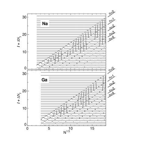
FIG. 5.: Filling of the orbitals with increasing cluster size $N$ in the self-consistent calculations for jellium clusters. $\Delta N_{l}$ is the change in the occupation of the orbitals with angular momentum $l$. In the plot, the $\Delta N_{l}$ are shifted by $l$. The small humps in the horizontal lines indicate a change in the occupation of an orbital with the corresponding angular momentum, i.e., the filling of that orbital. Since degenerate orbitals are filled simultaneously, the existence of several such humps for a given cluster size $N$ shows that the corresponding orbitals are degenerate. For the orbitals with large angular momentum these degeneracies are indicated by lines connecting such humps. The first hump for a given $l$ corresponds to the orbital with nodeless radial wave function $n=0$. Likewise, the orbital connected with the second hump has the quantum number $n=1$. As can be seen from the plots, the humps for orbitals with given $n$ are arranged into nearly straight lines of slightly different slope.

The main difference is that the pattern is shifted towards larger cluster sizes as the Wigner-Seitz radius decreases. We find that the first maximum in the shell amplitude is caused by the degeneracy of the states $\epsilon_{0,l}\approx\epsilon_{1,l-3}$ followed by $\epsilon_{0,l}\approx\epsilon_{2,l-6}$. The second maximum in the supershell structure is mainly due to the degeneracies $\epsilon_{1,l}\approx\epsilon_{2,l-3}$, supported by $\epsilon_{0,l}\approx\epsilon_{1,l-4}$ and $\epsilon_{1,l}\approx\epsilon_{3,l-6}$.

To find out why there are nodal regions in $\tilde{E}$, we first observe that the humps with a given quantum number $n$ are arranged into nearly straight lines (see Fig. 5). The slope of these occupation lines is larger for smaller $n$, i.e., the distance $\Delta l$ between two such lines increases with cluster size $N$. But since the angular momentum is

FIG. 6.: Position of the energy levels $\epsilon_{n,l}=\hbar^{2}k_{n,l}^{2}/2m$ in an infinite spherical potential well (spherical cavity) of radius $R_{0}$. For comparison with Fig. 5, we give $kR_{0}$ on the abscissa and the angular momentum $l$ on the ordinate. The position of the energy levels is indicated by crosses. For small $n$, these can be well described by the semiclassical expansion that is described in the text. The classical limit $L_{max}=\hbar k_{F}R_{0}$ is given by the dotted line.

quantized, degenerate energy levels exist only for integer values of $\Delta l$. Therefore regions where energy levels are degenerate are separated by regions without degeneracies. Hence the supershell structure can be traced back to the differences in the slopes of the occupation lines.

The origin of these lines can be understood from a simple classical argument. Assuming that the Fermi energy $E_{F}$ is fairly independent of the cluster size, the maximum angular momentum for an electron in a potential well of radius $R_{0}=r_{s}\,N^{1/3}$ is given by

$$L_{max}(N)=\hbar k_{F}\,R_{0},$$ (9)

where $\hbar k_{F}=(2mE_{F})^{1/2}$ is the Fermi momentum. Using semiclassical quantization, we can go beyond this crude approximation. The angular momentum is then written as $L=\hbar(l+1/2)$, where $l$ is the angular momentum quantum number. Introducing the parameter

$$\gamma={l+1/2\over k_{F}R_{0}},$$ (10)

which is unity in the classical case (9), the Bohr-Sommerfeld condition for an infinitely deep potential well of radius $R_{0}$ reads

$$\Big{(}l+{1\over 2}\Big{)}\left(\sqrt{{1\over\gamma^{2}}-1}-\arccos(\gamma)\right)=\pi\Big{(}n+3/4\Big{)}.$$ (11)

Expanding this equation to first order around the classical case $\gamma=1$, we can solve for the angular momentum of a state with quantum number $n$ at the Fermi level:

$$l+{1\over 2}\approx k_{F}R_{0}-{\Big{(}3\pi(n+3/4)\Big{)}^{2/3}\over 2}\,(k_{F}R_{0})^{1/3}.$$ (12)

Fig. 6 shows the angular momentum quantum number $l$ as a function of $k_{F}R_{0}$. It turns out that, for small quantum numbers $n$, the approximation (12) matches the quantum mechanical result quite well. The deviations for larger $n$ are due to the expansion around $\gamma=1$, not to the semiclassical approximation itself. Since a state $\epsilon_{n,l}$ at the Fermi level will be filled as the cluster size increases, the crosses in Fig. 6 can be identified with the humps in Fig. 5. Hence the expansion (12) provides, for small $n$, a good approximation to the occupation lines for the infinite potential well.

IV Scaling Analysis

In the present section we analyze the systematic variations in the shell and supershell structure as the jellium density is changed. The key to such an analysis is the identification of relevant scales. Expressing all data in terms of these scales, i.e. dealing with dimensionless reduced quantities, allows the results for different materials to be conveniently compared.

Obviously, the Wigner-Seitz radius $r_{s}$ is such a scale. It is a fundamental length describing how the volume of the cluster depends on the jellium density. Via the relation

$$k_{F}\approx\sqrt[3]{9\pi\over 4}\;{1\over r_{s}}$$

it is also related to a basic energy scale. As a simple example we note that the overall amplitude of the shell oscillations $\tilde{E}$ is proportional to $1/r_{s}^{2}$. This is shown in Fig. 7.

From the shape of the self-consistent Kohn-Sham potentials we can identify a second length scale. As can be seen from Fig. 8, for a given jellium density the shape FIG. 7.: Scaling of the amplitude of the shell oscillations with the electron density $n_{el}=3/(4\pi r_{s}^{3})$. The diamonds give the maximum amplitude of the oscillating part $\tilde{E}$ extracted from our self-consistent calculations. The dotted line gives a fit of these data points with the one-parameter function $const./r_{s}^{2}$.

FIG. 8.: Self consistent Kohn-Sham potential for sodium and gallium jellies of different sizes. To compare the surface region of the potentials, we chose $r$ minus the radius $R_{0}$ of the corresponding jellium as the abscissa. As can be seen, the shape of the potential at the surface of the clusters is fairly independent of the size $N$. The horizontal lines indicate the Fermi energies of the corresponding systems.

of the potentials around $R_{0}$ is quite independent of cluster size. For each material it can be characterized by the width of the surface region, which hence is a good candidate for an additional length scale. We will denote the surface width by $a$.

We might assume then that the changes in the electronic shells and supershells can be described in terms of the dimensionless parameter $a/r_{s}$. For a rough estimate of how $a$ varies with the jellium density, we have performed a simple Thomas-Fermi calculation for a plane jellium surface $n_{I}(z)=n_{I}\,\Theta(-z)$. Given an area $A$ the surface energy is

$$\sigma[n_{el}(z)]={\int\limits_{-\infty}^{\infty}\Big{(}\epsilon(n_{el}(z))\,n_{el}(z)-\epsilon(n_{I}(z))\,n_{I}(z)\Big{)}\,dz\over A},$$

where $\epsilon(n)$ is the Thomas-Fermi energy functional including the second order gradient correction to kinetic energy,[36] exchange energy and Hartree energy. To estimate $a$, we minimize the surface energy using a parametrized electron density, where the only parameter is the surface width

$$n_{el}(z)=n_{I}\,f(z/a).$$

A good choice for the function $f(z)$ is[37]

$$f(z)=\left\{\begin{array}[]{cl}1-{1\over 2}e^{z}&,\;z<0\\ {1\over 2}e^{-z}&,\;z\geq 0\;.\end{array}\right.$$

FIG. 9.: Width $a_{opt}$ of the surface region as a function of electron density. $a_{opt}$ was obtained from a Thomas-Fermi calculations (including gradient corrections and exchange) for a parametrized electron density. The energy functional included second-order gradient corrections to the kinetic energy, Coulomb energy, and exchange energy (full line). Including also exchange in the $X_{\alpha}$ approximation (Ref.[38]) yields the dotted curve.

The resulting surface width $a_{opt}$ as a function of the Wigner-Seitz radius $r_{s}$ is shown in Fig. 9. It is fairly independent of the jellium density, in agreement with the results of the self-consistent Kohn-Sham calculations shown in Fig. 8. Hence $r_{s}$ seems to be the only relevant length scale in the cluster problem.

The dependence of the shell and supershell structure on the scaling parameter $a/r_{s}$ is revealed by plotting the magic numbers and the supernodes against $1/r_{s}$. Fig. 10 shows the resulting pattern, which is surprisingly simple. The magic numbers are practically independent of the jellium density, while the supernodes are linearly shifted with $1/r_{s}$. A closer look at the supernodes reveals that their position can be accurately interpolated by a linear function. For some given jellium density a reliable estimate of the location of the minima in the supershell structure can be read off Fig. 11, without having to perform a time-consuming self-consistent calculation.

It is interesting to note that the first and the second supernode are shifted by the same amount. Writing the oscillating part of the total energy as a beating pattern

$$\tilde{E}(N) = \cos\Big{(}f_{1}N^{1/3}-\varphi_{1}\Big{)}+\cos\Big{(}f_{2}N^{1/3}-\varphi_{2}\Big{)}$$ (13)

$$= 2\;\cos\Big{(}{f_{1}-f_{2}\over 2}N^{1/3}-{\varphi_{1}-\varphi_{2}\over 2}\Big{)}$$ (15)

$$\times\cos\Big{(}{f_{1}+f_{2}\over 2}N^{1/3}-{\varphi_{1}+\varphi_{2}\over 2}\Big{)}$$

suggests a simple picture for understanding such a parallel displacement. Since the supershell oscillation is described by the first cosine in (15), the position of the $k^{th}$ supernode is given by

FIG. 10.: Position of the shell minima (crosses) and of the supernodes (diamonds) as a function of $1/r_{s}$. Corresponding shell minima and supernodes are connected by full and broken lines, respectively.

FIG. 11.: Shift of the first and second supernode as a function of $1/r_{s}$. The error bars are due to the uncertainty in determining the the envelope of $\tilde{E}(N)$. The lines give a linear fit of the data, the parameters of which are displayed in the plot.

$$N^{1/3}_{k}={(2k+1)\pi\over f_{1}-f_{2}}+{\varphi_{1}-\varphi_{2}\over f_{1}-f_{2}}.$$

In this picture a shift of the supernodes, which leaves the period of the oscillation unchanged, naturally arises from a variation of the phases $\varphi_{1}$ and $\varphi_{2}$. In a semiclassical approach, using a periodic orbit expansion,[3] these phases are determined by the cluster surface. This is consistent with the observation that the supershell structure is sensitive to the shape of the surface potential.[6, 23] Using an expansion of the relevant semiclassical integrals in terms of the scaling parameter $a/r_{s}$ (leptodermous expansion) it can be shown that the above interpretation indeed describes the mechanism underlying the observed shift of the supernodes.[39]

V Conclusions

We have analyzed how the oscillating part $\tilde{E}$ of the total energy extracted from self-consistent calculations depends on the electron density. It turns out that the magic numbers are fairly independent of the density, while the supershell oscillations are shifted towards larger cluster sizes as the Wigner-Seitz radius decreases. Focusing on the energy spectrum near the Fermi level $E_{F}$, we have found a simple pattern in which the orbitals are filled: the occupation lines. They can be understood using a semiclassical expansion. Qualitatively there is no difference between clusters of different density. The strong oscillations in $\tilde{E}$ are caused by degeneracies of energy levels close to $E_{F}$. The supershells are a consequence of the different slopes of the occupation lines, which imply transition zones between regions where levels are degenerate. The shift of the supernodes with increasing density can be understood from an analysis of the physical scales. We have identified $r_{s}$ as the relevant length scale for the cluster problem. It turns out that the location of the supernodes is linearly shifted with $1/r_{s}$.

Furthermore, the identification of $r_{s}$ as the typical length scale for the supershells suggests a justification of the ad hoc procedure proposed in Ref.[24] to improve the results of jellium calculations for gallium clusters. There it was found that the introduction of a non-homogeneous jellium background is essential for treating Ga_N clusters, while alkali-metal clusters are well described by a homogeneous jellium. With the help of the above scaling argument that puzzle may be resolved. Assuming that the typical length scale for features in the jellium is the ionic radius $r_{at}$, while the length scale for the electrons is the Wigner-Seitz radius $r_{s}$, we find that the importance of inhomogeneities increases with the number of valence electrons $Z_{val}\propto(r_{at}/r_{s})^{3}$. Hence, for trivalent materials a soft jellium surface should have a stronger influence on the supershells than for alkali metals.

REFERENCES

- [1] Present address: Department of Physics, University of Illinois at Urbana-Champaign, Urbana, IL 61801.
- [2] W. D. Knight, K. Clemenger, W. A. de Heer, W. A. Saunders, M. Y. Chou, and M. L. Cohen, Phys. Rev. Lett. 52, 2141 (1984).
- [3] H. Nishioka, K. Hansen, and B. R. Mottelson, Phys. Rev. B 42, 9377 (1990).
- [4] W. A. de Heer, Rev. Mod. Phys. 65, 611 (1993).
- [5] M. Brack, Rev. Mod. Phys. 65, 677 (1993).
- [6] K. Clemenger, Phys. Rev. B 44, 12991 (1991).
- [7] R. Balian and C. Bloch, Ann. Phys. (N.Y.) 69, 76 (1972).
- [8] M. C. Gutzwiller, J. Math. Phys. 11, 1791 (1970).
- [9] P. Stampfli and K. H. Bennemann, Z. Phys. D 25, 87 (1992).
- [10] J. Lermé, C. Bordas, M. Pellarin, B. Baguenard, J. L. Vialle, and M. Broyer, Phys. Rev. B 48, 9028 (1993).
- [11] P. Hohenberg and W. Kohn, Phys. Rev. 136, B864 (1964).
- [12] W. Kohn and L. J. Sham, Phys. Rev. 140, A1133 (1965).
- [13] R. O. Jones and O. Gunnarsson, Rev. Mod. Phys. 61, 689 (1989).
- [14] P. Ballone, W. Andreoni, R. Car, and M. Parinello, Europhys. Lett. 8, 73 (1989).
- [15] U. Röthlisberger and W. Andreoni, J. Chem. Phys. 94, 8129 (1991).
- [16] R. O. Jones, Phys. Rev. Lett. 67, 224 (1991).
- [17] D. Pines, Elementary Excitations in Solids (Benjamin, New York, 1964).
- [18] N. D. Lang and W. Kohn, Phys. Rev. B 1, 4555 (1970).
- [19] D. E. Beck, Solid State Commun 49, 381 (1984).
- [20] W. Ekardt, Phys. Rev. B 29, 1558 (1984).
- [21] K. Clemenger, Phys. Rev. B 32, 1359 (1985).
- [22] J. Lermé, M. Pellarin, E. Cottancin, B. Baguenard, J. L. Vialle, and M. Broyer, Phys. Rev. B 52, 14163 (1995).
- [23] J. Lermé, C. Bordas, M. Pellarin, B. Baguenard, J. L. Vialle, and M. Broyer, Phys. Rev. B 48, 12100 (1993).
- [24] M. Pellarin, B. Baguenard, C. Bordas, M. Broyer, J. Lermé, and J. L. Vialle, Phys. Rev. B 48, 17645 (1993).
- [25] J. Lermé, M. Pellarin, B. Baguenard, C. Bordas, J. L. Vialle, and M. Broyer, Phys. Rev. B 50, 5558 (1994).
- [26] J. Lermé, M. Pellarin, J. L. Vialle, and M. Broyer, Phys. Rev. B 52, 2868 (1995).
- [27] A. Hintermann and M. Manninen, Phys. Rev. B 27, 7262 (1983).
- [28] O. Genzken and M. Brack, Phys. Rev. Lett. 67, 3286 (1991).
- [29] O. Genzken, Mod. Phys. Lett. B 7, 197 (1993).
- [30] B. Baguenard, M. Pellarin, C. Bordas, J. Lermé, J. L. Vialle, and M. Broyer, Chem. Phys. Lett. 205, 13 (1993).
- [31] J. P. Perdew, J. A. Chevary, S. H. Vosko, K. A. Jackson, M. R. Pederson, D. J. Singh, and C. Fiolhais, Phys. Rev. B 46, 6671 (1992).
- [32] E. Engel and S. H. Vosko, Phys. Rev. B 47, 13164 (1993).
- [33] S. H. Vosko, L. Wilk, and M. Nusair, Can. J. Phys. 58, 1200 (1980).
- [34] E. Engel and J. P. Perdew, Phys. Rev. B 43, 1331 (1991).
- [35] D. M. Ceperley and B. J. Alder, Phys. Rev. Lett. 45, 566 (1980).
- [36] D. A. Kirzhnits, Zh. Eksp. Teor. Fiz. 32, 115 (1957) [Sov. Phys. JETP 5, 64 (1957)].
- [37] J. R. Smith, Phys. Rev. 181, 522 (1969).
- [38] J. C. Slater, The Self-consistent Field for Molecules and Solids (McGraw-Hill, New York, 1974), Vol. 4.
- [39] E. Koch, Phys. Rev. Lett. 76, 2678 (1996).
- [40] D. D. Johnson, Phys. Rev. B 38, 12807 (1988).