[

Common trends in the critical behavior of the Ising and directed walk models

Abstract

We consider layered two-dimensional Ising and directed walk models and show that the two problems are inherently related. The information about the zero-field thermodynamical properties of the Ising model is contained into the transfer matrix of the directed walk. For several hierarchical and aperiodic distributions of the couplings, critical exponents for the two problems are obtained exactly through renormalization.
cond-mat/9606118

]

The Ising model (IM) and the directed walk (DW) are among the most studied problems in lattice statistics. The IM is a standard model for magnetic or liquid-gas phase transitions whereas the DW can be used to describe linear fluctuating objects such as directed polymers, flux lines or interfaces in two-dimensional systems.

The IM is exactly solvable in two dimensions [2] and the solution can be generalized for layered systems with different types of distributions for the interlayer couplings such as periodic [3], quasi-periodic [4], aperiodic [5, 6] and random [7]. The DW is probably the simplest non-trivial problem in statistical mechanics for which exact results can be obtained on homogeneous [8], inhomogeneous [9] and random [10] lattices.

In this Letter, we present a hitherto unnoticed connection between the IM and the DW in two dimensions. Both problems are considered on layered lattices, such that the walk is directed along the translationally invariant direction. We show that the complete solution of the DW, i.e. the diagonalization of its transfer matrix (TM), provides all the necessary information to obtain the zero-field thermodynamical properties and correlation functions of the IM. The DW approach, which is simpler, is then used to perform an exact renormalization-group (RG) study of the TM eigenvalue problem for self-similar distributions of the couplings. The critical properties of the IM and DW are governed by two different fixed points of the same RG-transformation.

Let us first present the hidden relation between the two problems. We consider a layered IM in the extreme anisotropic limit [11]. The transfer matrix going in the direction parallel to the layers is $\exp(-\tau{\cal H})$, where $\tau$ is the lattice spacing in the Euclidian time direction, and ${\cal H}$ the Hamiltonian of a quantum Ising chain:

$${\cal H}=-{1\over 2}\sum_{k=1}^{L}h_{k}\,\sigma_{k}^{z}-{1\over 2}\sum_{k=1}^{L-1}J_{k}\,\sigma_{k}^{x}\sigma_{k+1}^{x}\;.$$ (1)

The $\sigma_{i}$s are Pauli spin operators, the transverse field $h_{k}=h$ plays the role of the temperature and the couplings $J_{k}$ are non-periodic.

Following Lieb et al [12] and Pfeuty [13] ${\cal H}$ can be transformed into a free-fermion model

$${\cal H}=\sum_{q=1}^{L}\Lambda_{q}(\eta_{q}^{\dagger}\eta_{q}-{1\over 2})$$ (2)

in terms of the fermion creation and annihilation operators $\eta_{q}^{\dagger}$, $\eta_{q}$. The fermion excitations $\Lambda_{q}$ are non-negative and satisfy the set of equations

$$\Lambda_{q}\Psi_{q}(k) = -h_{k}\Phi_{q}(k)-J_{k}\Phi_{q}(k+1)$$ (3)

$$\Lambda_{q}\Phi_{q}(k) = -J_{k-1}\Psi_{q}(k-1)-h_{k}\Psi_{q}(k)$$ (4)

with the boundary conditions $J_{0}=J_{L}=0$. The ${\bf\Phi}_{q}$s and ${\bf\Psi}_{q}$s, which are related to the coefficients of a canonical transformation, are normalized. They enter into the expressions of correlation functions and thermodynamical quantities [12, 13].

Usually one proceeds by eliminating either ${\bf\Psi}_{q}$ or ${\bf\Phi}_{q}$ in (4) and the excitations are deduced from the solution of an eigenvalue problem. This last step can be avoided by introducing a $2L$-dimensional vector ${\bf{V}}_{q}$ with components $V_{q}(2k-1)=-\Phi_{q}(k)$, $V_{q}(2k)=\Psi_{q}(k)$ and noticing that the relations in Eq. (4) correspond to the eigenvalue problem for the matrix

$$T=\left(\begin{array}[]{ccccccc}0&h_{1}&0&0&0&0&\cdots\\ h_{1}&0&J_{1}&0&0&0&\cdots\\ 0&J_{1}&0&h_{2}&0&0&\cdots\\ 0&0&h_{2}&0&J_{2}&0&\cdots\\ \vdots&\vdots&&\ddots&&\ddots&\end{array}\right)$$ (5)

which can be interpreted as the TM of a DW problem on two interpenetrating, diagonally layered square lattices. The walker makes steps with weights $h_{k}$ and $J_{k}$ between first-neighbour sites on one of the two lattices.

Changing ${\bf\Phi}_{q}$ into $-{\bf\Phi}_{q}$ in ${\bf{V}}_{q}$, the eigenvector corresponding to $-\Lambda_{q}$ is obtained. Thus all the information about the DW and the IM is contained into that part of the spectrum with $\Lambda_{q}\geq 0$. Later on we shall restrict ourselves to this sector.

Let us now consider the correlation lengths in the direction parallel to the layers for both problems. For the DW it can be expressed as a function of the two leading eigenvalues of the TM with:

$$\xi_{\parallel}^{\rm DW}=\left[\ln\left({\Lambda_{L}\over\Lambda_{L-1}}\right)\right]^{-1}\simeq{\Lambda_{L}\over\Lambda_{L}-\Lambda_{L-1}}\;.$$ (6)

Thus $\xi_{\parallel}^{\rm DW}$ is proportional to the inverse gap at the top of the spectrum. For the IM in the disordered phase the correlation length is the inverse of the lowest excitation energy of ${\cal H}$ in Eq. (2) so that

$$\xi_{\parallel}^{\rm IM}\sim\Lambda_{1}^{-1}\;.$$ (7)

$\Lambda_{1}$ is also the lowest eigenvalue in the spectrum of the TM. In the ordered phase $\Lambda_{1}=0$ and the correlation length involves the second eigenvalue $\Lambda_{2}$.

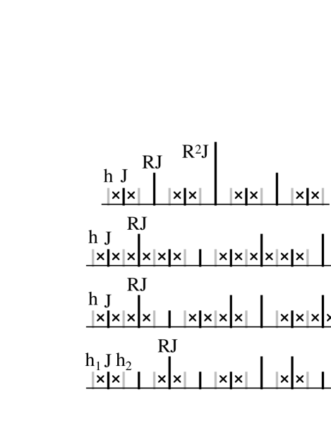
FIG. 1.: Matrix-elements $T_{j,j+1}$ as a function of $j$ for different non-periodic sequences: a) hierarchical b) period-doubling c) three-folding d) paper-folding. Components of the eigenvector to be decimated out in the RG transformation are denoted by crosses. The heights of solid vertical bars indicate the strength of the couplings, the grey bars stand for the field.

Approaching one of the two critical points, the correlation length of the problem is diverging and the corresponding part in the TM spectrum displays a scaling behavior. Let us consider a finite system with transverse size $L\gg 1$ and denote by $\Delta\Lambda_{i}$ either $\Lambda_{L}-\Lambda_{L-i}$ for the DW or $\Lambda_{i}$ itself for the IM with $i\ll L$. When lengths are rescaled by a factor of $b>1$, i.e. with $L^{\prime}=L/b$, the gaps are assumed to behave as

$$(\Delta\Lambda_{i})^{\prime}=b^{y_{\Lambda}}\Delta\Lambda_{i}\;,$$ (8)

where $y_{\Lambda}$ is the gap exponent which is generally different at different parts of the spectrum. This leads to the finite size behavior

$$\Delta\Lambda_{i}(L)\sim L^{-y_{\Lambda}}\;,$$ (9)

thus from Eqs. (6) and (7) the longitudinal correlation lengths are $\xi_{\parallel}\sim L^{y_{\Lambda}}$. Since $\xi_{\perp}\sim L$, the anisotropy exponent $z$, such as $\xi_{\parallel}\sim\xi_{\perp}^{z}$, is given by $z=y_{\Lambda}$. For the DW one is interested in the transverse fluctuations which are characterised by the wandering exponent $w$ through $\xi_{\perp}\sim\xi_{\parallel}^{w}$, thus $w=y_{\Lambda}^{-1}$.

The scaling properties of the spectrum of $T$ are conveniently studied using RG techniques. We consider different self-similar lattices for which exact RG transformations can be worked out so that we obtain exact results about the critical properties of both the IM and the DW. In the following the transverse field is assumed to be constant and equal to $h$.

Hierarchical sequence

We start with a hierarchical lattice in which the couplings $J_{k}$ follow the Huberman-Kerszberg sequence [14],

$$J_{k}=R^{n}J\,,\quad k=2^{n}(2m+1)\,,\quad n,m=0,1,\cdots\;,$$ (10)

with $0<R<1$. The eigenvalue problem for $T$ corresponds to the second order difference equations

$$T_{j,j-1}V(j-1)-\Lambda V(j)+T_{j,j+1}V(j+1)=0\;,$$ (11)

where $j=1,\cdots,2L$. To construct an exact recursion we eliminate from these equations components of the form $V(4l+2)$, $V(4l+3)$ which are connected to a $J$ coupling (indicated by crosses in Fig. 1a). After such a decimation the triplet $(h,J,h)$ is replaced by a renormalized field $h^{\prime}$ and keeping $R$ unchanged, the remaining couplings become $J^{\prime}=RJ$ due to the hierarchical structure of the sequence. Thus the renormalized equations keep the original form with $\Lambda$ changed into $\Lambda^{\prime}$. Introducing the reduced variables $\lambda=J/h$ and $\widehat{\Lambda}=\Lambda/h$ one arrives at the two-parameters recursion:

$$\widehat{\Lambda}^{\prime}={\widehat{\Lambda}\over\lambda}\,(\widehat{\Lambda}^{2}-\lambda^{2}-1)\;,\qquad\lambda^{\prime}=R\,(\widehat{\Lambda}^{2}-\lambda^{2})\;.$$ (12)

The RG-transformation has two non-trivial fixed points, governing the scaling of the eigenstates at the top of the spectrum (DW) and at $\Lambda=0$ (IM), respectively. The line $\widehat{\Lambda}=0$, corresponding to the IM situation, is invariant under the RG transformation in Eq. (12). Along this line, starting with a ferromagnetic model with $\lambda>0$, after one recursion step the system is transformed into an antiferromagnetic model with $\lambda<0$. The critical IM with $\lambda_{c}=1/R$ is transformed into the IM fixed point, which is situated at $\lambda^{*}=-1/R$. At the IM fixed-point the leading eigenvalue of the transformation is $\epsilon_{1}=R+1/R$ and the anisotropy exponent of the hierarchical IM is given by:

$$z=y_{\Lambda}={\ln(R+1/R)\over\ln 2}\;.$$ (13)

Thus scaling in the hierarchical IM close to the critical point is essentially anisotropic.

Scaling of the eigenstates at the top of the spectrum is governed by the DW fixed-point situated at

$$\lambda^{*}={R\over 1-R}\;,\qquad\widehat{\Lambda}\,^{*}={\sqrt{1-R+R^{2}}\over 1-R}\;,$$ (14)

and the leading eigenvalue is given by:

$$\epsilon_{1}={1\over R}+R+{1\over 2}+\left[\left({1\over R}+R+{1\over 2}\right)^{2}-2\right]^{1/2}\;.$$ (15)

Thus the wandering exponent of the walk is:

$$w={1\over y_{\Lambda}}={\ln 2\over\ln\epsilon_{1}}\;.$$ (16)

In the homogeneous model, with $R=1$, the DW fixed point is shifted to infinity since $\widehat{\Lambda}^{*}\to\infty$, $\lambda^{*}\to\infty$ and along the separatrix $\widehat{\Lambda}/\lambda\to 1$. To evaluate the scaling behavior we introduce new variables: $\kappa=1/\lambda$ and $\Delta=(\widehat{\Lambda}/\lambda)^{2}-1$, in terms of which the fixed point is given by $\kappa^{*}=0$ and $\Delta^{*}=0$. Then the separatrix is a straight line: $\Delta(\kappa)=a^{*}\kappa$, with $a^{*}=2$, and according to Eq. (12) one point of the $(\kappa,\Delta)$ plane with $\Delta=a\kappa$ will transform into $(\kappa^{\prime}=\kappa/a,\Delta^{\prime}=(1-2/a^{2})\Delta)$. Thus $a^{\prime}=a^{2}-2$ and the leading eigenvalue of the transformation is $\epsilon_{1}=4$, consequently $w=1/y_{\Lambda}=1/2$, in agreement with known results [8]. We note that $w(R)$ is discontinuous at $R=1$, since from Eq. (16) $\lim_{R\to 1_{-}}w(R)<1/2$.

Period-doubling sequence

In our next example, the couplings $J_{k}$ are generated according to the period-doupling sequence [15] which follows from the substitution $A\to AB$ and $B\to AA$. Here and in the following, the couplings are parametrized as $J_{A}=J$ and $J_{B}=RJ$.

In an exact RG transformation, six sites out of eight have to be decimated, as indicated on Fig. 1b. Associating new couplings $h^{\prime}$ with the decimated blocks one obtains a recursion in terms of $h^{\prime}$ and $\Lambda^{\prime}$ while $\lambda$ and $R\lambda$, thus the ratio $R$, remain unchanged. In terms of the reduced parameters the RG-transformation reads as

$$\widehat{\Lambda}^{\prime}={\widehat{\Lambda}\over R\lambda^{3}}(c-d)\;,\qquad\lambda^{\prime}={c\over R\lambda^{2}}\;,$$ (17)

with $c=\widehat{\Lambda}^{2}(-\widehat{\Lambda}^{2}+1+\lambda^{2})^{2}-R^{2}\lambda^{2}(\widehat{\Lambda}^{2}-\lambda^{2})^{2}$ and $d=(\widehat{\Lambda}^{2}-1)^{2}-\lambda^{2}\widehat{\Lambda}^{2}(1+R^{2})+\lambda^{2}(1+R^{2}\lambda^{2})$. The IM-fixed point of the transformation is at $\widehat{\Lambda}^{*}=0$ and $\lambda^{*}=-R^{-1/3}$, with the leading eigenvalue $\epsilon_{1}=(R^{1/3}+R^{-1/3})^{2}$. Since the rescaling factor of the transformation is $b=4$ we obtain

$$z={\ln(R^{1/3}+R^{-1/3})\over\ln 2}$$ (18)

for the anisotropy exponent of the period-doubling IM.

The top of the spectrum, corresponding to the DW problem, scales to a fixed point with $\widehat{\Lambda}\to\infty$, $\lambda\to\infty$, but $\widehat{\Lambda}/\lambda\to R$. In terms of the variables $\kappa=1/\lambda$ and $\Delta=(\widehat{\Lambda}/\lambda)^{2}-R^{2}$ the fixed-point is at $\kappa^{*}=0$ and $\Delta^{*}=0$, while the separatrix, close to the fixed point, is of the form $\Delta(\kappa)=a^{*}\kappa^{2}+O(\kappa^{4})$, with $a^{*}=(\sqrt{2}R-2R^{2})/(1-R^{2})$. Then, according to Eq. (17), a point of the ($\kappa,\Delta$)-plane with $\Delta=a\kappa^{2}$ will transform to $(\kappa^{\prime}\sim\kappa^{2},\Delta^{\prime}\sim\Delta^{1/2})$. This type of scaling behavior is compatible with an essential singularity in the gaps at the top of the spectrum,

$$\Delta\Lambda_{i}\sim\exp(-CL^{\sigma})$$ (19)

with $\sigma=1/2$, since the rescaling factor is $b=4$. Thus the parallel correlation length of the DW is given by $\xi_{\parallel}^{\rm DW}\sim\exp(CL^{1/2})$ and the transverse fluctuations of the walk grow anomalously, on a logarithmic scale:

$$\left<\left[X(t)-X(0)\right]^{2}\right>^{1/2}\sim\ln^{2}(t)\;.$$ (20)

Here $X(t)$ denotes the position of the walker at time $t$. We note that the same asymptotic behavior is found in the Sinai model [16] of a one-dimensional random walk in a random environment.

Three-folding sequence

The three-folding sequence is generated by the substitutions $A\to ABA$, $B\to ABB$ [17]. In the RG transformation - as indicated on Fig. 1c - blocks of four sites are decimated out. Due to the asymmetric nature of the blocks, after one RG step the transfer matrix becomes asymmetric, too: $T_{j,j+1}/T_{j+1,j}=s$ for $j$ even, while $T_{j,j+1}/T_{j+1,j}=s^{-1}$ for $j$ odd.

The recursion relations in this case are more conveniently expressed using the variables $\widetilde{\Lambda}=\Lambda/J$, $\mu=h/J$ and $s$, while $R$ remains unchanged:

$$\widetilde{\Lambda}^{\prime}=\widetilde{\Lambda}\left[\left(1-{c\over e}\right)\left(1-{d\over e}\right)\right]^{1/2}\;,\quad\mu^{\prime}=\mu^{3}{R\over e}\;,$$ (21)

with $c=\mu^{2}(\widetilde{\Lambda}^{2}-\mu^{2}-R^{2})$, $d=\mu^{2}(\widetilde{\Lambda}^{2}-\mu^{2}-1)$ and $e=(\widetilde{\Lambda}^{2}-1)(\widetilde{\Lambda}^{2}-R^{2})-\mu^{2}\widetilde{\Lambda}^{2}$. We note that the asymmetry parameter $s$, such that $s^{\prime}=s(c-e)(d-e)$, does not enter into the recursions for $\widetilde{\Lambda}$ and $\mu$.

At the IM fixed point ($\widetilde{\Lambda}^{*}=0,~{}\mu^{*}=R^{1/2}$) the leading eigenvalue of the RG transformation is $\epsilon_{1}=[(2+R)(2+R^{-1})]^{1/2}$, thus the anisotropy exponent is given by

$$z={\ln(2+R)(2+R^{-1})\over 2\ln 3}\;.$$ (22)

The DW fixed point is again at infinity: $\widetilde{\Lambda}^{*}=\infty$, $\mu^{*}=\infty$, with $\widetilde{\Lambda}^{*}/\mu^{*}=1$. The scaling behavior at this fixed point is similar to that in the period-doubling case. The eigenvalues at the top of the spectrum show an essential singularity like in Eq. (19) with $\sigma=1/2$ and the transverse fluctuations grow on a logarithmic scale as in Eq. (20).

Paper-folding sequence

Finally, we consider the paper-folding sequence [17] which is generated by the two-letter substitutions $AA\to AABA$, $AB\to AABB$, $BA\to ABBA$ and $BB\to ABBB$. In the RG transformation, decimating out blocks of two sites (Fig. 1d), alternating field variables $h_{1}$ and $h_{2}$ are generated for odd and even lattice sites, respectively. Furthermore, the transfer-matrix becomes asymmetric and the asymmetry parameters are different for odd and even elements. As a consequence, the exact RG transformation contains altogether six parameters. Here we just present the scaling behavior at the two non-trivial fixed points, details of the calculation will be presented elsewhere [18].

At the IM fixed point, the anisotropy exponent is continuously varying and given by:

$$z={\ln(1+R)(1+R^{-1})\over\ln 4}\;.$$ (23)

At the DW fixed point the scaling is again of the streched exponential form with a leading behaviour for transverse fluctuations given by Eq. (20).

Let us now turn to a discussion of the critical behavior we have obtained for the IM and the DW. All the aperiodic IMs we considered are strongly anisotropic with a continuously varying anisotropy exponent. In the extended parameter space there is a line of fixed points parametrized by the coupling ratio $R$. The critical behavior of the DWs is also found to be anomalous: the lines of fixed points of the non-periodic systems are disconnected from the fixed point of the homogeneous ones. For the hierarchical model the wandering exponent is discontinuous at $R=1$ whereas for the other sequences the transverse fluctuations grow on the same logarithmic scale.

The difference between the IM and the DW on the same lattice can be understood using a relevance-irrelevance criterion [5] which is a counterpart for aperiodic systems of the Harris criterion [19] for random ones. The cross-over exponent associated with a layered non-periodic perturbation is [5] $\phi=1+\nu(\Omega-1)$ where $\nu$ is the exponent of the correlation length, perpendicular to the layers, for the unperturbed system and $\Omega$ is a wandering exponent [20] which characterizes the fluctuations in the couplings $J_{k}$ around their average $\overline{J}$ as $\sum_{k=1}^{L}(J_{k}-\overline{J})\sim L^{\Omega}$.

All the non-periodic sequences we considered have $\Omega=0$. For the IM with $\nu=1$ the cross-over exponent vanishes. Thus the perturbation is marginal, which explains the continuous variation of the anisotropy exponent. On the other hand, for the anisotropic DW with $\nu_{\perp}=1/2$, the cross-over exponent is $\phi=1/2$ and the perturbation is relevant. This is again in agreement with our results.

- [1] Permanent address: Research Institute for Solid State Physics, P.O. Box 49, H-1525 Budapest, Hungary and Institute of Theoretical Physics, Szeged University, H-6720 Szeged, Hungary.
- [2] L. Onsager, Phys. Rev. 65, 117 (1944).
- [3] M. E. Fisher, J. Phys. Soc. Jap. Suppl. 26, 87 (1968); H. Au-Yang and B. M. McCoy, Phys. Rev. B 10, 886 (1974); P. Hoever, W. F. Wolff and J. Zittartz, Z. Phys. B 44, 129 (1981).
- [4] C. A. Tracy, J. Phys. A 21, L603 (1988); F. Iglói, J. Phys. A 21, L911 (1988); G. V. Benza, Europhys. Lett. 8, 321 (1989).
- [5] J. M. Luck, J. Stat. Phys. 72, 417 (1993).
- [6] L. Turban, F. Iglói and B. Berche, Phys. Rev. B 49, 12695 (1994); F. Iglói and L. Turban, Europhys. Lett. 27, 91 (1994); B. Berche, P-E. Berche, M. Henkel, F. Iglói, P. Lajkó, S. Morgan and L. Turban, J. Phys. A 28, L165 (1995); F. Iglói, P. Lajkó and F. Szalma, Phys. Rev. B 52, 7159 (1995); P-E. Berche, B. Berche and L. Turban, J. Physique I 6, 621 (1996); F. Iglói and P. Lajkó (unpublished).
- [7] B. M. McCoy and T. T. Wu, Phys. Rev. 176, 631 (1968); B. M. McCoy, Phys. Rev. B 2, 2795 (1970); L. V. Mikheev and M. E. Fisher, Phys. Rev. B 49, 378 (1994); D. S. Fisher, Phys. Rev. B 51, 6411 (1995).
- [8] M. E. Fisher, J. Chem. Soc. Faraday Trans. 82, 1569 (1986).
- [9] C. L. Henley and R. Lipowsky, Phys. Rev. Lett. 59, 1679 (1987); A. Garg and D. Levine, Phys. Rev. Lett. 59, 1683 (1987).
- [10] B. Derrida, Physica Scripta T38, 6 (1991); M. Kardar, in Fluctuating Geometries in Statistical Mechanics and Field Theory, Les Houches Summer School (1994) cond-mat/9411022.
- [11] J. Kogut, Rev. Mod. Phys. 51, 659 (1979).
- [12] E. Lieb, T. Schultz and D. Mattis, Ann. Phys. (N. Y.) 16, 407 (1961).
- [13] P. Pfeuty, Ann. Phys. (Paris) 57, 79 (1970).
- [14] B. A. Huberman and M. Kerszberg, J. Phys. A 18, L331 (1985).
- [15] P. Collet and J. P. Eckmann, Iterated Maps in the Interval as Dynamical Systems (Birkhäuser, Boston, 1980).
- [16] Ja. G. Sinai, Theor. Prob. Appl. 27, 247 (1982).
- [17] M. Dekking, M. Mendès-France and A. van der Poorten, Math. Intelligencer 4, 130 and 190 (1983).
- [18] F. Iglói and L. Turban (unpublished).
- [19] A. B. Harris, J. Phys. C 7, 1671 (1974).
- [20] M. Queffélec, Substitutional Dynamical Systems–Spectral Analysis, Lecture Notes in Mathemathics, Vol. 1294, edited by A. Dold and B. Eckmann (Springer, Berlin, 1987).