[

Conduction band spin splitting and negative magnetoresistance in ${\rm A}_{3}{\rm B}_{5}$ heterostructures.

Abstract

The quantum interference corrections to the conductivity are calculated for an electron gas in asymmetric quantum wells in a magnetic field. The theory takes into account two different types of the spin splitting of the conduction band: the Dresselhaus terms, both linear and cubic in the wave vector, and the Rashba term, linear in wave vector. It is shown that the contributions of these terms into magnetoconductivity are not additive, as it was traditionally assumed. While the contributions of all terms of the conduction band splitting into the D’yakonov–Perel’ spin relaxation rate are additive, in the conductivity the two linear terms cancel each other, and, when they are equal, in the absence of the cubic terms the conduction band spin splitting does not show up in the magnetoconductivity at all. The theory agrees very well with experimental results and enables one to determine experimentally parameters of the spin-orbit splitting of the conduction band.

]

It was first found by Dresselhaus [1] in 1955 that in cubic crystals with symmetry $T_{d}$ there is a spin splitting of the conduction band, which is cubic in the electron wave vector $k$. This splitting is described by the Hamiltonian[2, 3]:

$$H_{s}= \gamma\sum_{i}\sigma_{i}k_{i}\left(k_{i+1}^{2}-k_{i+2}^{2}\right),$$ (2)

$$\left(i=x,y,z;\quad i+3\rightarrow i\right),$$

where $\sigma_{i}$ are the Pauli matrices (in this paper we take $\hbar=1$ everywhere except in final formulas). If the symmetry of a crystal is reduced, the splitting linear in wave vector appears, for example, in uniaxial crystals [4], in $T_{d}$ crystals under a deformation[5, 6], and, most importantly, in quantum wells and heterostructures [6, 7, 8, 9, 10]. In symmetric quantum wells grown along $[001]$, the conduction band Hamiltonian has the form:

$$H={k^{2}\over 2m^{*}}+\left(\mbox{\boldmath$\sigma$}{\bf\Omega}\right),$$ (3)

where $\mbox{\boldmath$\sigma$}=(\sigma_{x},\sigma_{y})$, ${\bf\Omega}=(\Omega_{x},\Omega_{y})$ are two-dimensional vectors with components in the plane of the quantum well. Here the spin splitting coefficients ${\bf\Omega}$ are proportional to the bulk coefficient $\gamma$ in Eq. (2). According to Ref. [11],

$$\Omega_{x} = -\Omega_{1}^{(1)}\cos\varphi-\Omega_{3}\cos 3\varphi,$$ (4)

$$\Omega_{y} = \ \Omega_{1}^{(1)}\sin\varphi-\Omega_{3}\sin 3\varphi,$$ (5)

$$\Omega_{1}^{(1)} = \gamma k\left(\left\langle k_{z}^{2}\right\rangle-{1\over 4}k^{2}\right),\quad\Omega_{3}=\gamma{k^{3}\over 4},$$ (6)

where $k^{2}=k_{x}^{2}+k_{y}^{2}$, $\tan\varphi=k_{x}/k_{y}$, and $\left\langle k_{z}^{2}\right\rangle$ is the average wave vector in the direction $z$, normal to the quantum well.

In asymmetric quantum wells, or in the presence of a deformation $\epsilon_{xy}$, the Hamiltonian $H$ includes another, so-called Rashba term[8]:

$$H^{\prime}=\alpha[\mbox{\boldmath$\sigma k$}]_{z}.$$ (7)

This term can be included in the Hamiltonian Eq. (3) if one includes additional terms into ${\bf\Omega}$:

$$\Omega_{x}=\Omega_{1}^{(2)}\sin\varphi,\quad\Omega_{y}=-\Omega_{1}^{(2)}\cos\varphi,\quad\Omega_{1}^{(2)}=\alpha k.$$ (8)

In deformed crystals, according to Refs. [5, 6, 12],

$$\alpha={1\over 2}C_{3}\epsilon_{xy}.$$ (9)

The values of the coefficient $C_{3}$ for some ${\rm A}_{3}{\rm B}_{5}$ compounds are given in Refs. [6, 12]. In an asymmetric quantum well the coefficient $\alpha$ is proportional to the average value of the electric field (or potential gradient) in the well. This coefficient was calculated in the framework of the $\mbox{\boldmath$k$}\cdot\mbox{\boldmath$p$}$ method [13, 14], neglecting the immediate vicinity of the potential barriers. However, if the effective mass approximation would have been valid throughout the entire well, including the barriers, then $\alpha=0$.

If the linear in $k$ spin splitting is given by only one of the terms Eq. (5) or Eq. (8), all observable effects are identical, because these two Hamiltonians can be converted one into the other by a unitary transformation. In both cases the conduction band minimum is shaped like a ring around $k=0$. However, if both terms are present, the electron spectrum changes qualitatively: the energy minima now occur at finite $k$ along the axes $(110)$ or $(1\bar{1}0)$, depending on the signs of $\Omega_{1}^{(1)}$ and $\Omega_{1}^{(2)}$.

Both terms Eq. (5) and Eq. (8) give additive contributions into the D’yakonov–Perel’ spin-relaxation rate[9]:

$${1\over\tau_{s_{xx}}}={1\over 2\tau_{s_{zz}}}=2\left(\Omega_{1}^{2}\tau_{1}+\Omega_{3}^{2}\tau_{3}\right),$$ (10)

where $\Omega_{1}^{2}={\Omega_{1}^{(1)}}^{2}+{\Omega_{1}^{(2)}}^{2}$ and $\tau_{n}$, $n=1,3$, is the relaxation time of the respective component of the distribution function:

$${1\over\tau_{n}}=\int W(\vartheta)\left(1-\cos n\vartheta\right)\,d\vartheta.$$ (11)

Here $W(\vartheta)$ is the probability of scattering by an angle $\vartheta$.

In this paper we show that such additivity does not exist for weak localization effects, which are responsible for the negative magnetoresistance (NMR). In the theory of the NMR the spin splitting of the conduction band was first taken into account in Ref. [7]. In this paper it was supposed that the magnetoconductivity $\Delta\sigma(B)$ depends only on the spin relaxation times, by analogy with the Larkin-Hikami-Nagaoka theory[15], which considered the Elliott-Yafet spin-relaxation mechanism. In Ref. [11] it was shown that for D’yakonov–Perel’ spin relaxation this approach is valid when Hamiltonian Eq. (3) contains only cubic in $k$ terms, the ones with $\Omega_{3}$ (note also that the spin relaxation rates, given in Ref. [7], should be increased two times[11]). The formulas derived in Ref. [11] can be used if only one of the terms Eq. (5) or Eq. (8) is present in the Hamiltonian Eq. (3).

When both terms Eq. (5) or Eq. (8) coexist in the conduction band Hamiltonian, one can reduce the equation for the Cooperon propagator ${{\rm\kern 2.40005pt\vrule width=0.50003pt,height=6.02773pt,depth=-0.21529pt\kern-2.59995ptC}}_{0}(\mbox{\boldmath$q$})$, as described in Ref. [11], using the iteration in the parameters $\Omega_{i}\tau_{0}$ and $\mbox{\boldmath$q$}\mbox{\boldmath$v$}\tau_{0}$, where $\tau_{0}^{-1}=\int W(\vartheta)\,d\vartheta$ is the elastic lifetime and $v$ is the Fermi velocity, to the following form:

$${\cal H}{{\rm\kern 2.40005pt\vrule width=0.50003pt,height=6.02773pt,depth=-0.21529pt\kern-2.59995ptC}}_{0}={1\over 2\pi\nu_{0}\tau_{0}^{2}},$$ (12)

where $\nu_{0}$ is the density of states at the Fermi level and

$${\cal H}= {1\over\tau_{\varphi}}+{1\over 2}v^{2}q^{2}\tau_{1}+$$ (17)

$$\left(\Omega_{1}^{2}\tau_{1}+\Omega_{3}^{2}\tau_{3}\right)\left(2+\sigma_{x}\rho_{x}+\sigma_{y}\rho_{y}\right)+$$

$$2\left(\sigma_{x}\rho_{y}+\sigma_{y}\rho_{x}\right)\Omega_{1}^{(1)}\Omega_{1}^{(2)}\tau_{1}+$$

$$v\tau_{1}\left[\left(\sigma_{x}+\rho_{x}\right)\left(-\Omega_{1}^{(1)}q_{x}+\Omega_{1}^{(2)}q_{y}\right)+\right.$$

$$\left.\left(\sigma_{y}+\rho_{y}\right)\left(\Omega_{1}^{(1)}q_{y}-\Omega_{1}^{(2)}q_{x}\right)\right].$$

The components of the matrix ${{\rm\kern 2.40005pt\vrule width=0.50003pt,height=6.02773pt,depth=-0.21529pt\kern-2.59995ptC}}_{0}$ are determined by two pairs of spin indices, and the matrices $\sigma$ act on the first pair, while the matrices $\rho$, also Pauli matrices, - on the second pair. The magnetic fiend dependent correction to the conductivity is determined by the quantity $S(\mbox{\boldmath$q$})$ [11]:

$$\Delta\sigma=-{e^{2}D\over 4\pi^{3}}\int\limits_{0}^{q_{max}}S(\mbox{\boldmath$q$})\,d^{2}q$$ (18)

where $q_{max}^{2}=(D\tau_{1})^{-1}$, $D=v^{2}\tau_{1}/2$ is the diffusion coefficient, and

$$S(\mbox{\boldmath$q$})=2\pi\nu_{0}\tau_{0}^{2}\sum_{\alpha\beta}{{\rm\kern 2.40005pt\vrule width=0.50003pt,height=6.02773pt,depth=-0.21529pt\kern-2.59995ptC}}_{0_{\alpha\beta\beta\alpha}}=-{1\over{\cal E}_{0}}+\sum^{1}_{m=-1}{1\over E_{m}},$$ (19)

${\cal E}_{0}$ and $E_{m}$ are the eigenvalues of the operator ${\cal H}$, corresponding to the eigenfunctions $\phi_{0}$ (antisymmetric singlet state) and $\phi_{l}^{m}$ with $l=1$, $m=-1,0,1$ (symmetric triplet state). The singlet contribution is the same as in Ref. [11]:

$${\cal E}_{0}=Dq^{2}+{1\over\tau_{\varphi}}.$$ (20)

The values $E_{m}$ are the eigenvalues of the matrix operator

$$\tilde{\cal H}= Dq^{2}+{1\over\tau_{\varphi}}+2\left(\Omega_{1}^{2}\tau_{1}+\Omega_{3}^{2}\tau_{3}\right)\left(2-J_{z}^{2}\right)-$$ (24)

$$4i\Omega_{1}^{(1)}\Omega_{1}^{(2)}\tau_{1}\left(J_{+}^{2}-J_{-}^{2}\right)+$$

$$2(D\tau_{1})^{1/2}\left[-\Omega_{1}^{(1)}\left(J_{+}q_{+}+J_{-}q_{-}\right)+\right.$$

$$\left.i\Omega_{1}^{(2)}\left(J_{+}q_{-}-J_{-}q_{+}\right)\right].$$

Here $J_{i}$ are the matrices of the angular momentum operator with total momentum $L=1$, $J_{\pm}=(J_{x}\pm iJ_{y})/\sqrt{2}$, and $q_{\pm}=q_{x}\pm iq_{y}$.

An interesting particular case occurs when $\Omega_{1}^{(1)}=\pm\Omega_{1}^{(2)}$ and $\Omega_{3}=0$. If one introduces new coordinates (upper sign for $\Omega_{1}^{(1)}=+\Omega_{1}^{(2)}$ and lower sign for $\Omega_{1}^{(1)}=-\Omega_{1}^{(2)}$)

$$v={x\pm y\over\sqrt{2}},\ u={x\mp y\over\sqrt{2}},$$ (25)

$$q_{v}={q_{x}\pm q_{y}\over\sqrt{2}},\ q_{u}={q_{x}\mp q_{y}\over\sqrt{2}},$$ (26)

$$J_{v}={J_{x}\pm J_{y}\over\sqrt{2}},\ J_{u}={J_{x}\mp J_{y}\over\sqrt{2}},$$ (27)

it is easy to show that the operator $\tilde{\cal H}$ in these coordinates becomes

$$\tilde{\cal H} = D\left[q_{v}^{2}+\left(q_{u}-q_{u0}J_{v}\right)^{2}\right]+{1\over\tau_{\varphi}},$$ (28)

$$q_{u0}^{2} = {4\Omega_{1}^{2}\tau_{1}\over D}$$ (29)

In the basis of eigenfunctions of $J_{v}$ we have three independent equations for eigenvalues $E_{m}$:

$$E_{m}=D\left[q_{v}^{2}+\left(q_{u}+mq_{u0}\right)^{2}\right]+{1\over\tau_{\varphi}}.$$ (30)

In this case $S(\mbox{\boldmath$q$})$ becomes

$$S(\mbox{\boldmath$q$})= \left\{D\left[q_{v}^{2}+\left(q_{u}+q_{u0}\right)^{2}\right]+{1\over\tau_{\varphi}}\right\}^{-1}+$$ (32)

$$\left\{D\left[q_{v}^{2}+\left(q_{u}-q_{u0}\right)^{2}\right]+{1\over\tau_{\varphi}}\right\}^{-1}.$$

When calculating the conductivity Eq. (18), one can neglect the shift in $q$-space $q_{u0}$ compared to $q_{max}$ on the upper limit of the integral. The result for the conductivity correction is:

$$\Delta\sigma=-{e^{2}\over 2\pi^{2}\hbar}\ln{\tau_{\varphi}\over\tau_{1}}.$$ (33)

Note that in order for the diffusion approximation itself to be valid, the condition $\tau_{\varphi}\gg\tau_{1}$ must hold. One can see that when $\Omega_{1}^{(1)}=\pm\Omega_{1}^{(2)}$ and $\Omega_{3}=0$, $\Delta\sigma$ is determined by the same formula as without any spin relaxation. Note that the spin relaxation rate Eq. (10) does not show any peculiar behavior in this case.

The reason for such a striking difference between NMR and spin relaxation can be seen if one writes the Hamiltonian $H^{\prime}=\mbox{\boldmath$\sigma$}{\bf\Omega}$ at $\Omega_{1}^{(1)}=\pm\Omega_{1}^{(2)}$ and $\Omega_{3}=0$ in the form

$$H^{\prime}=2\alpha(\sigma_{v}k_{u}),$$ (34)

where the coordinates $u$ and $v$ are determined by Eq. (26). Then one can see that the random “effective magnetic field” $2\alpha k_{u}$, parallel to axis $v$, leads to the random precession of electron spin in the plane, perpendicular to this axis. The frequency of this rotation is proportional to $k_{u}$, or to the velocity $V_{u}$. During the time $\delta t$ between two consecutive scattering acts the spin rotates by an angle $\varphi_{21}$, proportional to the distance $V_{u}\delta t=u_{2}-u_{1}$. Therefore, the total angle of the spin precession along a path between points with coordinates $u_{0}$ and $u_{n}$ is proportional to the length $L_{n}=u_{n}-u_{0}$. For the spin relaxation, these paths can be anything and resulting spin rotations are random. On the other hand, the NMR is determined only by the trajectories for which $L_{n}$ is smaller than the electron wavelength, i.e. $L_{n}=0$ within the framework of our theory. Hence, for $\Omega_{1}^{(1)}=\pm\Omega_{1}^{(2)}$ and $\Omega_{3}=0$ the total spin rotation on the trajectories which contribute into the NMR is zero[16] When $\Omega_{1}^{(1)}=\pm\Omega_{1}^{(2)}$, but $\Omega_{3}\neq 0$, the direction of the random magnetic field changes with the direction of $k$, and the total spin rotation on a closed trajectory is not zero any more. The absence of a spin contribution to interference effects in one-dimensional metal rings for a spin Hamiltonian, similar to Eq. (34), has been pointed out in Refs. [10, 17], where the conductivity oscillations and universal fluctuations of the conductance were considered.

In a magnetic field $q_{\pm}$ become operators and can be expressed through the operators $a^{\dagger}$ and $a$, which increase and decrease the Landau level number $n$[11]:

$$D^{1/2}q_{+}=\delta^{1/2}a,\quad D^{1/2}q_{-} = \delta^{1/2}a^{\dagger},\quad Dq^{2}=\delta\{aa^{\dagger}\},$$ (35)

$$\{aa^{\dagger}\} = {1\over 2}(aa^{\dagger}+a^{\dagger}a),$$ (36)

where

$$\delta={4eBD\over\hbar c}.$$ (37)

The non-zero matrix elements of these operators are

$$\left\langle n-1\right|a\left|n\right\rangle = \left\langle n\right|a^{\dagger}\left|n-1\right\rangle=\sqrt{n},$$ (38)

$$\left\langle n\right|\{aa^{\dagger}\}\left|n\right\rangle = n+{1\over 2}.$$ (39)

The magnetic field dependent correction to the conductivity Eq. (18) now becomes

$$\Delta\sigma=-{e^{2}\delta\over 4\pi^{2}\hbar}\sum_{n=0}^{n_{max}}\left(-{1\over{\cal E}_{0n}}+\sum_{m=-1}^{1}{1\over E_{mn}}\right),$$ (40)

where $n_{max}=1/\delta\tau_{1}$. According to Eqs. (20,24,36),

$${\cal E}_{0n}=\delta\left(n+{1\over 2}\right)+{1\over\tau_{\varphi}},$$ (41)

and $E_{mn}$ are the eigenvalues of the operator

$$\tilde{\cal H}= \delta\{aa^{\dagger}\}+{1\over\tau_{\varphi}}+2\left(\Omega_{1}^{2}\tau_{1}+\Omega_{3}^{2}\tau_{3}\right)\left(2-J_{z}^{2}\right)-$$ (44)

$$4i\Omega_{1}^{(1)}\Omega_{1}^{(2)}\tau_{1}\left(J_{+}^{2}-J_{-}^{2}\right)+2(\delta\tau_{1})^{-1}$$

$$\left[-\Omega_{1}^{(1)}\left(J_{+}a-J_{-}a^{\dagger}\right)+i\Omega_{1}^{(2)}\left(J_{+}a^{\dagger}-J_{-}a\right)\right].$$

One can see that in the general case, when both $\Omega_{1}^{(1)}$ and $\Omega_{1}^{(2)}$ are non-zero, the determinant of $\tilde{\cal H}$ can no longer be split into submatrices $3\times 3$ in the basis of functions $\left|n,m\right\rangle$ ($m=-1,0,1$), unlike Eq. (10) of Ref. [11]. Therefore, the only way to find eigenvalues $E_{mn}$ is to diagonalize numerically the matrix $\tilde{\cal H}$. The number of elements one has to take for a given value of magnetic field $B$, or $\delta$, is at least $n_{max}$ and increases infinitely as $B$ approaches $\mathrm{𝟎}$. Note that the size of the matrix $\tilde{\cal H}$ is $N=3n_{max}$.

The numerical diagonalization of the matrix $\tilde{\cal H}$ was performed using the LAPACK eigensolver for hermitian banded matrices. To improve convergence of the sum in Eq. (40), we add and subtract from each $1/E_{mn}$ its approximate asymptotic value $1/\delta(n+1)$ at large $n$ (the constant, $1$, added to $n$ is needed only to extend summation to $n=0$, as in Eq. (40)). The sum of terms $\delta E_{mn}^{-1}-(n+1)^{-1}$ can be extended to $n\rightarrow\infty$, while the sum of added terms $(n+1)^{-1}$ can be replaced by an integral. Both approximations cause errors proportional to $\tau_{1}/\tau_{\varphi}$, $(\Omega_{i}\tau_{i})^{2}$, and $1/n_{max}$, but the very approach of this paper is valid only when this parameter is small and $n_{max}$ is very large. Therefore, we use the following expression for the magnetoconductivity:

$$\Delta\sigma= -{e^{2}\over 4\pi^{2}\hbar}\left\{\sum_{n=0}^{\infty}\left[-{\delta\over{\cal E}_{0n}}+{1\over n+1}\right]+\right.$$ (47)

$$\sum_{n=0}^{\infty}\sum_{m=-1}^{1}\left[{\delta\over E_{mn}}-{1\over n+1}\right]-$$

$$2\ln(\delta\tau_{1})-2C\Biggr{\}},$$

where $C$ is the Euler constant. In order to compute the sum of $1/E_{mn}$ to $n=\infty$ numerically, we perform the calculations for few values of $n_{max}$ in the range from 500 to 5000 and extrapolate to $n\rightarrow\infty$.

FIG. 1.: Dimensionless magnetoconductivity $\Delta\bar{\sigma}$ vs dimensionless magnetic field $\bar{\delta}$ (Eq. (52)) for $H_{SO}/H_{\varphi}=4$ and $\Omega_{1}^{(2)}=0$ (a) and $\Omega_{1}^{(1)}=\Omega_{1}^{(2)}$ (b). For both plots (a) and (b) the curves 1 through 5 show dependencies at different $H^{\prime}_{SO}/H_{SO}=1$, 3/4, 1/2, 1/4, and 0, respectively.

We now present the results of the numerical computations. Let us introduce the following characteristic magnetic fields[11]:

$$H_{\varphi} = {c\hbar\over 4eD\tau_{\varphi}},\ {B\over H_{\varphi}}=\delta\tau_{\varphi},$$ (48)

$$H_{SO} = {c\hbar\over 4eD}\left(2\Omega_{1}^{2}\tau_{1}+2\Omega_{3}^{2}\tau_{3}\right),\ H^{\prime}_{SO}={c\hbar\over 4eD}2\Omega_{1}^{2}\tau_{1},$$ (49)

$$H^{(1)}_{SO} = {c\hbar\over 4eD}{2\Omega_{1}^{(1)}}^{2}\tau_{1},\ H^{(2)}_{SO}={c\hbar\over 4eD}{2\Omega_{1}^{(2)}}^{2}\tau_{1}.$$ (50)

Note that the field $H_{SO}$ is proportional to the spin relaxation rate. We also use dimensionless units for the conductivity and magnetic field:

$$\bar{\delta} \equiv {B\over H_{\varphi}}=\delta\tau_{\varphi},$$ (51)

$$\Delta\bar{\sigma} = {4\pi^{2}\hbar\over e^{2}}\left(\Delta\sigma-\lim_{\delta\rightarrow 0}\Delta\sigma\right).$$ (52)

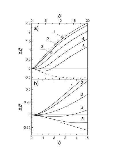
FIG. 2.: Dimensionless magnetoconductivity $\Delta\bar{\sigma}$ vs dimensionless magnetic field $\bar{\delta}$ (Eq. (52)) for $H_{SO}/H_{\varphi}=4$ and for $H^{\prime}_{SO}/H_{SO}=1$ ($\Omega_{3}=0$). The curves 1 through 5 show dependencies at different ratios $H^{(1)}_{SO}/H^{\prime}_{SO}=1/2$, 5/8, 3/4, 7/8, and 1, respectively. Lower plot shows magnification of small magnetic fields region. The dashed curve shows the dependency for $\Omega_{1}=0$.

We begin by demonstrating the effect of the coexistence of both terms $\Omega_{1}^{(1)}$ and $\Omega_{1}^{(2)}$ in the spin splitting. In Fig. 1a we reproduce the results of Ref. [11] for magnetoconductivity at $H_{SO}/H_{\varphi}=4$ and different $H^{\prime}_{SO}/H_{SO}$. These results can be obtained from Eqs. (40-44) if one leaves only $\Omega_{1}^{(1)}$, or $\Omega_{1}^{(2)}$, and sets the other one to 0. Our results have better numerical accuracy, especially for small $\bar{\delta}$, due to extrapolation to $n\rightarrow\infty$ in the sum Eq. (47). Note that the lowest curve, with $H^{\prime}_{SO}=0$, gives the result of the Larkin-Hikami-Nagaoka theory[15]. In Fig. 1b we show the curves for the same values of $H_{SO}/H_{\varphi}$ and $H^{\prime}_{SO}/H_{SO}$, but now $\Omega_{1}^{(1)}=\Omega_{1}^{(2)}$. The effect of redistribution of the spin splitting between $\Omega_{1}^{(1)}$ and $\Omega_{1}^{(2)}$ is, naturally, more pronounced for large $H^{\prime}_{SO}/H_{SO}$, when the linear in $k$ term dominates the spin relaxation. One can see that for $H^{\prime}_{SO}/H_{SO}>0.5$ the results in Fig. 1 a and b are qualitatively different: the magnetoresistance minimum shifts closer to $B=0$ and eventually disappears, and $\Delta\sigma$ becomes monotonic.

This effect is shown in more details in Fig. 2, where the magnetoconductivity is plotted for $H^{\prime}_{SO}/H_{SO}=1$ and various $H^{(1)}_{SO}/H^{\prime}_{SO}$. The lowest solid curve reproduces the result of Ref. [11]. One can clearly see the shift of magnetoconductivity minimum and its disappearance when $\Omega_{1}^{(1)}$ and $\Omega_{1}^{(2)}$ become comparable ($H^{(1)}_{SO}/H^{\prime}_{SO}$ close to $1/2$). The minimum disappears and the slope of magnetoconductivity at $B=0$ changes sign at $H^{(1)}_{SO}/H^{\prime}_{SO}\approx 3/4$.

FIG. 3.: Dimensionless magnetoconductivity $\Delta\bar{\sigma}$ vs dimensionless magnetic field $\bar{\delta}$ (Eq. (52)) for $H_{SO}/H_{\varphi}=4$ and for $H^{\prime}_{SO}/H_{SO}=1/2$. The curves 1, 2, 3 correspond to $H^{(1)}_{SO}/H^{\prime}_{SO}=1/2$, 3/4, and 1, respectively. The dashed curve shows the dependency for $\Omega_{1}=0$.

While redistribution of linear in $k$ spin splitting between the Dresselhaus term Eq. (5) and the Rashba term Eq. (8) has maximum effect on the magnetoconductivity when the linear splitting is dominant, the quantitative effects of such redistribution can be seen when linear and cubic splittings are comparable. In Fig. 3 the dependence of magnetoconductivity on $H^{(1)}_{SO}/H^{\prime}_{SO}$ is shown for $H^{\prime}_{SO}/H_{SO}=1/2$, when the contributions of both linear and cubic terms to the spin relaxation rate are equal. One can see that, while the effect is not as dramatic as in Fig. 2, it has qualitatively the same character.

We now return to the question of the cancellation of the Rashba and Dresselhaus terms in linear spin splitting. One can see that the cancellation of spin relaxation terms in conductivity, which occurs when $\Omega_{1}^{(1)}=\Omega_{1}^{(2)}$ and $\Omega_{3}=0$, also happens in a magnetic field. In this case the eigenvalue equation Eq. (44) splits into three independent equations, analogous to Eq. (30). The commutation relations for the operators $q_{u}$ and $q_{v}$ in a magnetic field do not change with the shift of $q_{u}$ by a constant value $q_{u0}$ in each of these equations:

$$D\left[q_{v},q_{u}\pm q_{u0}\right]=-i\,{\delta\over 2}.$$ (53)

Therefore, all eigenvalues $E_{mn}$ are equal to ${\cal E}_{0n}$, and

$$\Delta\bar{\sigma}=-2\left[\psi\left({1\over 2}+{H_{\varphi}\over B}\right)-\ln{H_{\varphi}\over B}\right],$$ (54)

where $\psi$ is a digamma-function.

FIG. 4.: Cancellation of linear terms in spin splitting. Dimensionless magnetoconductivity $\Delta\bar{\sigma}$ is plotted vs dimensionless magnetic field $\bar{\delta}$ (Eq. (52)) for constant $\Omega_{3}^{2}\tau_{3}\tau_{\varphi}=1/2$ for plot a) and $2$ for plot b), and for different $H^{\prime}_{SO}/H_{\varphi}$. Solid lines show the magnetoresistance when $\Omega_{1}^{(1)}=\Omega_{1}^{(2)}$ (maximum cancellation), dashed lines are for $\Omega_{1}^{(2)}=0$ (no cancellation). For each family of curves (solid or dashed) $H^{\prime}_{SO}/H_{\varphi}$ takes values 0, 1, 2, 3, and 4, with 0 for the uppermost curve and 4 for the lowest curve (at $H^{\prime}_{SO}$ solid and dashed curves coincide).

As we have already noted, this cancellation of terms with $\Omega_{1}^{(1)}$ and $\Omega_{1}^{(2)}$ occurs only when $\Omega_{3}=0$. However, it is reasonable to suppose that addition of a small cubic splitting will break this cancellation only slightly, resulting in a very weak dependence of the magnetoconductivity on $\Omega_{1}$ when $\Omega_{1}^{(1)}=\Omega_{1}^{(2)}$. Fig. 4 shows that it is indeed so. In Fig. 4a the magnetoconductivity is presented for small $\Omega_{3}$ and different $\Omega_{1}$. One can see that when $\Omega_{1}^{(1)}=\Omega_{1}^{(2)}$ (solid lines in Fig. 4), the magnetoconductivity practically does not change when $H^{\prime}_{SO}/H_{\varphi}$ changes from $\mathrm{𝟎}$ to $4$. This shows that the two terms in linear splitting almost cancel each other in NMR, and the result looks as if there were no linear splitting at all, even though the latter can be much larger that the cubic splitting. On the other hand, the same change in $H^{\prime}_{SO}/H_{\varphi}$ has very strong effect on $\Delta\sigma$ when only one of the linear splitting terms is present ($\Omega_{1}^{(2)}=0$, dashed lines). Fig. 4b shows that the same trend persists even for large cubic splittings, though the effect becomes less dramatic. We must stress again that no such cancellation occurs in the spin relaxation rates, which are sensitive only to the total spin splitting.

The cancellation discussed above is more than an abstract curiosity. The Rashba term Eq. (7) in quantum wells can be changed by deformation. For a $[001]$ quantum well, a deformation along $(110)$ or $(1\bar{1}0)$ will, according to Eq. (9) change the coefficient $\alpha$ in Eq. (7). The resulting splitting can exceed the contribution Eq. (3) for not too high deformations[12]. Such an experiment would allow independent measurement of the magnitudes of linear and cubic in $k$ spin splittings Eq. (5), as well as the sign and magnitude of the part of the coefficient $\alpha$, which is determined by the well asymmetry.

We should also note that the recent paper Ref. [14] contains discussion of the contributions of two types of linear spin splitting: the Rashba term and the Dresselhaus term. The authors of Ref. [14] have used spin-orbit splittings, calculated in Ref. [18]. These splittings were derived from the experimental data, using the formulas from Ref. [7], which implies an assumtion that splitting of both types give additive contributions to NMR, similar to their contribution to spin relaxation time. The results presented above show that in fact the situation is exactly opposite: the appearance of splitting of the second type decreases, rather than increases, the total contribution of linear splitting to NMR. This contribution continues to decrease until both terms in linear splitting becomes equal.

As far as comparison of theory and experiment is concerned, no good agreement had been achieved for quantum wells (unlike the NMR in metal films, where the theory provides very accurate description of experimental results). The theory of Refs. [7, 13] was unable to describe the experimental results of Refs. [18, 19] in a wide range of magnetic fields[14, 18]. The main reason for the discrepancy between experiment and theory was the assumption that linear and cubic terms give additive contributions to the magnetoresistance and the formula of Ref. [7] can be used for the D’yakonov–Perel’ spin relaxation mechanism. It was first shown in Ref. [11] that this assumption is incorrect; however, no comparison with experiment was presented in this paper. We now proceed to illustrate that the new theory is able to describe magnetoconductivity in semiconductor quantum wells quite accurately.

FIG. 5.: Comparison of theoretical and experimental results for the magnetoconductivity. Squares show the experimental results of Ref. 18. Solid line shows the best fit obtained from our theory, fitting parameters are $H_{\varphi}=0.028\;{\rm Gs}$, $H_{SO}/H_{\varphi}=31$, $H^{\prime}_{SO}/H_{\varphi}=28.5$, and $H^{(1)}_{SO}/H_{\varphi}=26$. The best fit with only one term in linear splitting is shown by the dashed line, fitting parameters are $H_{SO}/H_{\varphi}=26$ and $H^{\prime}_{SO}/H_{\varphi}=23.5$. The fits for $\Omega_{1}=0$ are shown by doted lines. It is not possible to fit the experiment in the whole range of magnetic fields in this case. The fit which works best to the left of the magnetoconductivity minimum (marked by $l$) has $H_{SO}/H_{\varphi}=6.7$ (this is the value found in Ref. 18), the fit to the right side of the minimum (marked by $r$) has $H_{SO}/H_{\varphi}=4$.

In Fig. 5 we show the comparison of the experimental results from Ref. [18] with the theory presented in this paper. The main difficulty in obtaining a well-defined fit arises from the cancellation of the two terms in the linear splitting, discussed above. Indeed, the best fit, shown in Fig. 5 by the solid line, is obtained for ${\Omega_{1}^{(1)}}^{2}\tau_{1}\tau_{\varphi}=13$, ${\Omega_{1}^{(2)}}^{2}\tau_{1}\tau_{\varphi}=1.25$, and ${\Omega_{3}}^{2}\tau_{3}\tau_{\varphi}=1.25$. If one wants to find the best fit with only one term in the linear splitting of the conduction band, the fitting parameters are ${\Omega_{1}^{(1)}}^{2}\tau_{1}\tau_{\varphi}=11.75$, $\Omega_{1}^{(2)}=0$, and ${\Omega_{3}}^{2}\tau_{3}\tau_{\varphi}=1.25$, and the agreement is also very good. Comparison of the two sets of fitting parameters above shows that the addition of the second term in linear splitting, with $\Omega_{1}^{(2)}$, almost cancels a part of the first term, with $\Omega_{1}^{(1)}$. The effect is that the main dependence of the magnetoconductivity on the linear splitting can be described by the parameter $\left({\Omega_{1}^{(1)}}^{2}-{\Omega_{1}^{(2)}}^{2}\right)\tau_{1}\tau_{\varphi}$, and an equal increase of both $\Omega_{1}^{(1)}$ and $\Omega_{1}^{(2)}$ makes only a small difference. On the other hand, an attempt to fit the experiment with the formula of Ref. [7], which can be used for $\Omega_{1}=0$, fails: one can see in Fig. 5 that it is possible to fit the magnetoconductivity either on the right of the minimum or on the left, but not in the whole range of the magnetic field. The cancellation of the linear splitting, shown above, emphasizes the importance of magnetoconductivity measurements under a deformation, where the ratio of the linear splitting terms can be controlled independently.

Using values of the characteristic magnetic fields Eq. (49), determined from the fit, we can estimate the coefficients $\gamma$ and $\alpha$ of the spin-orbit Hamiltonian Eqs. (2,7). From Eq. (5),

$$\gamma={\hbar\Omega_{1}^{(1)}\over k\left(\left\langle k_{z}^{2}\right\rangle-{1\over 4}k^{2}\right)}.$$ (55)

Here we should take $k$ equal to the Fermi wave vector $k_{F}=\sqrt{\,2\pi N_{s}}$, and $\left\langle k_{z}^{2}\right\rangle$ can be estimated using the Fang-Howard wave function [20] for the electrons in the heterostructure:

$$\psi(z)=\sqrt{\,{b^{3}\over 2}}\,z\>{\rm e}^{-bz/2}.$$ (56)

Then $\left\langle k_{z}^{2}\right\rangle=b^{2}/4$. The parameter $b$ is determined mainly by the density of the electron gas. We can estimate $b$, using the simple expression, given in Ref. [21]:

$$b=\left({16.5\pi e^{2}mN_{s}\over\kappa\hbar^{2}}\right)^{1/3}\!\!\!\!,$$ (57)

where $\kappa$ is the dielectric constant and $m$ is the electron effective mass.

From the fit in Fig. 5 we have the value ${\Omega_{1}^{(1)}}^{2}\tau_{1}\tau_{\varphi}\approx 13$. The product $\tau_{1}\tau_{\varphi}$ can be found from the value of the magnetic field $H_{\varphi}\approx 0.028\;{\rm Gs}$, because, according to Eq. (49),

$$H_{\varphi}={c\hbar\over 4eD\tau_{\varphi}}={c\hbar\over 2v_{F}^{2}e\tau_{1}\tau_{\varphi}},$$ (58)

where $v_{F}=\hbar k_{F}/m$ is the Fermi velocity of electrons. Using the electron density $N_{s}=6.1\>10^{11}\;{\rm cm}^{-2}$ from Table 1 of Ref. [18], the electron mass in GaAs $m=0.067m_{0}$, and the dielectric constant of GaAs $\kappa=12.55$, we obtain the following estimate:

$$\gamma\approx 25\;{\rm eV\;\AA^{3}}.$$ (59)

This value for $\gamma$ agrees surprisingly well with the results, obtained in Ref. [12] from the measurements of spin relaxation using optical orientation.

The fit also allows to estimate the coefficient $\alpha$ of the Rashba term:

$$\alpha={\hbar\Omega_{1}^{(2)}\over k_{F}}.$$ (60)

Using the value ${\Omega_{1}^{(1)}}^{2}\tau_{1}\tau_{\varphi}\approx 1.25$ we get the estimate

$$\alpha\approx 1.2\;{\rm meV\;\AA}.$$ (61)

The value of the coefficient $\alpha$ had never been measured, and, as we noted before, it would have been exactly 0 in non-deformed quantum wells if the effective mass approximation were working everywhere, including the interface. Authors of Refs. [13, 14] have estimated this coefficient, assuming that the interface gives no contribution at all, for a uniform electric field in the quantum well:

$$\alpha_{\rm theor}={\hbar^{2}\over 2m}{\Delta\over E_{g}}{2E_{g}+\Delta\over(E_{g}+\Delta)(3E_{g}+2\Delta)}\,eE,$$ (62)

where $E_{g}$ is the direct band gap, $\Delta$ is the spin-orbit energy splitting, $E$ is the electric field. In a heterostructure the electric field changes in the $z$ direction from $4\pi N_{s}e/\kappa$ at the interface to practically 0 on the other side of the electron gas. In this case it should be replaced by an average electric field

$$\langle E\rangle=\int\limits_{0}^{\infty}E(z)\,|\psi(z)|^{2}\ dz,$$ (63)

where $E(z)$ itself is determined by the distribution of electron density:

$$E(z)={4\pi eN_{s}\over\kappa}\left(1-\int\limits_{0}^{z}|\psi(z^{\prime})|^{2}\ dz^{\prime}\right).$$ (64)

We have taken the following values for the energy gaps of GaAs:[22] $E_{g}=1.42\;{\rm eV}$ and $\Delta=0.33\;{\rm eV}$. Substitution of Eqs. (63,64) into Eq. (62) yields the estimate

$$\alpha_{\rm theor}=2.2\;{\rm meV\;\AA}.$$ (65)

This number is about twice the value which fits the experiment. We believe this is quite reasonable agreement considering the fact that the estimate Eq. (62) is really an upper bound, because it neglects the contribution of the field in the interface, and the latter tends to decrease $\alpha$. On the other hand, if one assumes $\alpha=2.2\;{\rm meV\;\AA}$ and uses the cancellation effect discussed above to add equal corrections to $\Omega_{1}^{(1)}$ and $\Omega_{1}^{(2)}$, this will result in a fit nearly as good as the one we suggested. For this new fit $\gamma$ changes to approximately $28\;{\rm eV\;\AA^{3}}$, and the change is well within the accuracy of existing determination of $\gamma$.

Finally, we can use the value of $\Omega_{3}^{2}\tau_{3}\tau_{\varphi}=1.25$ to estimate the ratio $\tau_{3}/\tau_{1}$. From Eq. (5) it follows that

$${\Omega_{3}\over\Omega_{1}^{(1)}}={4\left(\left\langle k_{z}^{2}\right\rangle-{1\over 4}k_{F}^{2}\right)\over k_{F}^{2}},$$ (66)

which gives the value

$${\tau_{3}\over\tau_{1}}\approx{1\over 4}.$$ (67)

Theoretically, this ratio can vary from $1/9$ for small-angle scattering (like scattering on remote charged impurities) to $1$ for short-range scattering. For a structure with fairly large mobility, $\mu\approx 1.1\>10^{5}\;{\rm cm}^{2}/{\rm V\;sec}$, the value $1/4$ is not unreasonable.

In conclusion, we have presented a new, improved theory for quantum interference corrections to the conductivity of an electron gas in a semiconductor quantum well in a magnetic field. The theory is valid for D’yakonov–Perel’ spin relaxation and when the phase relaxation time $\tau_{\varphi}$ is much longer than the momentum relaxation time $\tau_{1}$, so that the diffusion approximation can be used. Our theory correctly takes into account the contributions of different terms in spin splitting of the conduction band. We have shown that while the spin relaxation rate depends only on the total magnitude of the spin splitting, the different parts of the latter give non-additive contributions into the magnetoresistance. Furthermore, the two terms in the linear in wave vector part of the spin splitting, known as Rashba and Dresselhaus terms, actually cancel each other when their magnitudes are comparable. Using the new theory we were able to fit the experimental data for the magnetoconductivity in a wide range of magnetic fields. The spin–orbit splitting coefficient for the conduction band, obtained from the fit, is in very good agreement with the one measured in optical orientation experiments.

Lastly, we would like to note that the spin splitting leads to similar interference corrections to magnetoconductivity of hopping conductors[23]. We expect that in this case it is also important to distinguish between different terms in the spin Hamiltonian, whose contributions to NMR will not be additive.

We are grateful to J. Allen and D. Hone for helpful comments. The authors acknowledge support by the San Diego Supercomputer Center, where part of the calculations were performed. The research was supported in part by the Soros Foundation (G. E. P.) and by the Center for Quantized Electronic Structures (QUEST) of UCSB (F. G. P.).

REFERENCES

[1] G. Dresselhaus, Phys. Rev. 100, 580
(1955).
[2] E. I. Rashba and V. I. Sheka, Sov. Phys. — Sold
State, 3, 1257 (1961).
[3] M. I. D’yakonov and V. I. Perel’, JETP 33,
1053 (1971).
[4] E. I. Rashba and V. I. Sheka, Fiz. Tverd. Tela,
additional collection II, 162 (1959).
[5] G. L. Bir and G. E. Pikus, Fiz. Tverd. Tela, 3,
3050(1961).
[6] E. L. Ivchenko and G. E. Pikus, “Superlattices
and other heterostructures: symmetry and optical phenomena”, Springer
series in solid state sciences, 110, Springer-Verlag, Berlin,
Heidelberg, 1994.
[7] B. L. Altshuler, A. G. Aronov, A. I. Larkin, and
D. E. Khmelnitskii, JETP 54, 411 (1981).
[8] Yu. L. Bychkov and E. I. Rashba, J. Phys. C 17, 6093 (1984).
[9] M. I. D’yakonov, Y. Yu. Kachorovskii, Sov. Phys.
Semicond. 20, 110 (1986).
[10] Yu. B. Lyanda-Geller, A. D. Mirlin, Phys. Rev.
Lett. 72, 1894 (1994).
[11] S. V. Iordanskii, Yu. B. Lyanda-Geller, G. E.
Pikus, JETP Letters 60, 206 (1994).
[12] G. E. Pikus and A. Titkov, “Spin Relaxation under
Optical orientation”, in “Optical Orientation”, ed. by F. Mayer and
B. Zakharchenya, North Holland, Amsterdam (1984).
[13] G. Lommer, F. Malcher, and U. Rössler, Phys. Rev.
Lett. 60, 728 (1988).
[14] E. A. de Andrada e Silva, G. C. LaRocca, and F.
Bassani, Phys. Rev. B. 50, 8523 (1994).
[15] S. Hikami, A. Larkin, Y. Nagaoka, Progr. Theor.
Phys. 63, 707 (1980).
[16] We are grateful to M. I. D’yakonov, who had
directed our attention to this difference between closed and open
trajectories for the D’yakonov-Perel’ spin relaxation mechanism.
[17] A. V. Aronov and Yu. B. Lyanda-Geller,
unpublished.
[18] D. P. Dresselhaus, C. Papavassillion, R.
Wheeler, and R. Sacks, Phys. Rev. Lett. 68, 106 (1992);
[19] J. E. Hansen et. al, Phys. Rev. B 47,
16040 (1993).
[20] F. F. Fang and W. E. Howard, Phys. Rev. Lett., 16, 797 (1966).
[21] T. Ando, A. B. Fowler, and F. Stern, Rev. Mod. Phys.,
54, 437 (1982).
[22] Landolt–Börnstein New Series, Vol. 17a:
“Physics of group IV elements and III–V compounds”, ed. by O.
Madelung, Springer-Verlag, Berlin, Heidelberg (1982).
[23] T. V. Shakhbazyan and M. E. Raikh, Phys. Rev. Lett.
73, 1408 (1994).