Transfer and Decay of an Exciton Coupled to Vibrations in a Dimer

Abstract

Transfer and decay dynamics of an exciton coupled to a polarization vibration in a dimer is investigated in a mixed quantum-classical picture with the exciton decay incorporated by a sink site. Using a separation of time scales, it is possible to explain analytically the most important characteristics of the model.

If the vibronic subsystem is fast, these are the enhancement of nonlinear self trapping due to the sink and the slowing down of the exciton decay for large coupling or sink strength. Numerical results obtained recently for the DST approximation to the model are quantitatively explained and new dynamic effects beyond this approximation are found.

If the vibronic subsystem is slow, the behavior of the system follows closely the predictions of the adiabatic approximation. In this regime, the exciton decay crucially depends on the initial conditions of the vibronic subsystem.

In the transition regime between adiabatic and DST approximation, complex dynamics is observed by numerical computation. We discuss the correspondence to the chaotic behavior of the excitonic-vibronic coupled dimer without trap.

I Introduction

The purpose of this paper is to study the interplay between a coherent transfer regime of an exciton and two processes leading to the loss of the linear character of the exciton transfer, namely trapping of the exciton at a sink site with a prescribed sink rate $\Gamma$ and the coupling to intramolecular polarization vibrations.

A lot of work has been done on exciton transfer theories during the last decades. Beginning with the microscopic treatment by Haken and Reineker [1] and Grover and Silbey [2] a number of theories such as the Continuous Time Random Walk (CTRW) [3], the Pauli Master equation (PME) [4], the Generalized Master equation (GME) [5], the Stochastic Liouville equation (SLE) and the Haken-Strobl-Reineker (HSR) model (see [6] and references therein) were developed and mainly directed to obtaining equations which describe the coupled coherent and incoherent motion of the excitation. The investigation of exciton transfer on relatively small molecular aggregates such as dimers or triades is of much interest for clarifying the applicability of exciton transfer theories to experimental situations such as described in [7, 8].

Trapping of quasiparticles due to a sink site constitutes an important phenomenon in many molecular systems. In photosynthesis, for instance, an exciton in a harvesting antenna transfers its energy to a reaction center, where it can be trapped. Electron transfer processes then follow. Pearlstein and his coworkers were the first who recognized that the consequences of a sink on the energy transfer processes are different in the coherent and incoherent regimes [9] (and references therein). Čápek and Szöcs [10] pointed out the necessity of a transformation of the memory functions in the presence of a sink. They also gave a prescription for a proper inclusion of the sink into the HSR model. This found application e. g. in computer simulations of the excitation transfer in photosynthetic systems [11, 12]. Recently, a new form of purely coherent memory functions in presence of a sink was derived and shown to have important consequences for the excitation transfer [13]. New memory functions were also used to obtain characteristics entering the CTRW description in the presence of a sink [14].

The coupling between electronic and vibronic degrees of freedom in molecular and condensed media is another basic mechanism influencing transfer properties of electronic excitations in these systems. The investigation of its consequences started from the polaron problem in solid states (see e. g. [15] and references therein; for exciton-phonon interaction see [16]) and continued with the study of the influence of the vibronic bath variables on the excitation transfer properties in the framework of the generalized Master equation [5] and stochastic Liouville equation approaches [6].

With the development of the theory of dynamical systems it has become attractive to analyze the implications of electronic-vibronic couplings employing concepts and methods of this field. Using such a dynamic system approach we study the detailed picture of the time evolution of a small number of relevant variables of the system, which are assumed to interact weakly with the environment. Recent experimental developments in the field of ultrashort time resolved spectroscopy (see e. g. [17]) seem to make a direct observation of this time evolution possible in the near future.

In the present paper we focus our interest on the exciton dynamics in a molecular dimer coupled to intramolecular vibrations. A remarkable feature of this model is the possibility of self trapping, i. e. unequal time averaged occupation probabilities on the two sites of the configuration. The easiest way to obtain this effect from a coupling to vibrational degrees of freedom leads to the two-site discrete self trapping (DST) equation [18, 19, 20] which is a nonlinear but self contained equation of motion for the excitonic site occupation amplitudes. More sophisticated approaches take the dynamics of the vibrations explicitly into account by using a mixed quantum-classical description [21, 22] or by treating the coupled system quantum mechanically [23]. Another interesting point is the effect of dissipation on self trapping [24, 25, 26].

Although the influences of vibronic coupling and trapping on transport properties have been investigated separately in great detail, the combination of both, which can be important in the application of transfer theory, has rarely been addressed in the past. In a recent paper [27] we have studied the interplay between vibrational coupling and trapping due to a sink site for a dimer and a trimer in the framework of the DST approximation. An extension of the results seems to be possible into two directions. One can either try to describe larger molecular aggregates within the same framework or one can try to improve the dynamic model which is used. In this paper we will adopt the latter way and take account of the dynamics of a particular vibronic variable, too. For this purpose the coupled excitonic-vibronic system will be treated in a mixed quantum-classical description [21, 22], which is justified whenever the quantum fluctuations in the vibronic subsystem are negligible. The model we use will be specified and developed further in section II, where we also indicate the modifications that lead to the DST equation.

The explicit introduction of a vibronic degree of freedom makes not only the dynamics of the system more complex, it also increases the number of initial conditions that have to be specified in order to uniquely determine a solution. Motivated by the experimental situation e. g. in photosynthetic units, the creation of the exciton will always be assumed at the site without sink. For the vibronic degrees of freedom we will consider various possibilities. As we shall see, the initial conditions can crucially influence the dynamics and it is not easy to overlook all the dynamical regimes the model is capable of from numerical computations only. Therefore we devote section III to an analytical treatment of the system assuming some separation between the different time scales. In particular, we will generalize the analysis of the fixed points for the excitonic-vibronic coupled dimer without sink [22] to the present system. This will provide a global picture of the phase space which we shall further support in section IV by discussing the time dependence of the total occupation probability and the relative site occupation probabilities for some specific solutions.

The results of section III will also allow for a quantitative understanding of the DST dimer with sink. One of our aims is to study what is inherited in our more complex model from this approximation and which dynamic effects are beyond it. We will therefore briefly recall the relevant numerical results from [27] and discuss them in the light of our findings in section III A.

Since the mixed quantum-classical description we are using in this paper can be justified best for small oscillator frequencies, we pay much attention to this adiabatic regime, too. As we shall see, the assumption of slow vibrations is just the antipode of the DST case and therefore new dynamic effects different from DST results can be expected from it.

II Description of the Model

A The Hamiltonian

We consider the dynamics of an exciton moving on a molecular dimer. At each of the two monomers the exciton is allowed to interact with an intramolecular vibronic degree of freedom. Thus, the Hamiltonian of our model contains excitonic, vibronic and interaction parts denoted by $H_{\rm exc}$, $H_{\rm vib}$ and $H_{\rm int}$, respectively:

$$H=H_{\rm exc}+H_{\rm vib}+H_{\rm int},$$ (1)

$H_{\rm exc}$ describes a two site model

$$H_{\rm exc}=\sum_{n}\epsilon_{n}c_{n}^{*}c_{n}+\sum_{n\neq m}V_{nm}c_{n}^{*}c_{m}$$ (2)

with $n,m\;=\;1,2$. $c_{n}$ is the probability amplitude of the exciton to occupy the n-th molecule and $V_{nm}$ the transfer matrix element due to dipole-dipole interaction. In a standard two site model, the $\epsilon_{i}$ are real quantities and correspond to the local site energies of the exciton. Here, we allow $\epsilon_{2}$ to contain a negative imaginary part in order to describe the decay of the exciton on the sink site 2. Since we are not interested in the effect of a site energy difference on the exciton dynamics here, we set

$$\epsilon_{1}=0\hskip 28.45274pt\epsilon_{2}=-i{\Gamma\over 2},$$ (3)

which is equivalent to the extended sink model for the exciton decay introduced in [10] on the density matrix level. This model has been shown to solve the problem of a consistent description of exciton trapping at a sink meeting basic physical requirements such as positive occupation probabilities.

The vibrational part $H_{\rm vib}$ is taken as the sum of the energies corresponding to intramolecular vibrations at each of the monomers for which we use the harmonic approximation

$$H_{\rm vib}=\sum_{n}\frac{1}{2}(p_{n}^{2}+\omega_{n}^{2}q_{n}^{2}).$$ (4)

Here $q_{n},p_{n}$ and $\omega_{n}$ are the coordinate, the canonic conjugate momentum and the frequency of the intramolecular vibration of the $n$-th molecule, respectively.

The interaction Hamiltonian takes into account that the exciton energy depends on the molecular configuration of the monomers which is expressed by the coordinates $q_{n}$. Using a first order expansion in $q_{n}$ one has

$$H_{\rm int}=\sum_{n}\gamma_{n}q_{n}c_{n}^{*}c_{n},$$ (5)

where $\gamma_{n}$ are some coupling constants. In order to restrict the number of free parameters as much as possible we will assume that the dimer is symmetric except for the additional sink term on site 2, i. e. $\omega_{1}=\omega_{2}=\omega$, $\gamma_{1}=\gamma_{2}=\gamma$ and $V_{12}=V_{21}=-V$.

In what follows we will use a mixed quantum-classical description of the dynamics, i. e. we treat the vibronic degrees of freedom in the classical approximation while retaining the quantum wave function for the excitonic two site system. This approximation can be justified over a finite time range which increases as the oscillator frequencies and coupling constants decrease. When it exceeds the life time of the exciton the mixed quantum-classical picture describes correctly the decay of the excitation.

Using units with $\hbar=1$ we obtain from (1)-(5) the equations of motion

$$i\,d/dt\,{c}_{1} = \gamma q_{1}c_{1}-V\,c_{2}$$ (6)

$$i\,d/dt\,{c}_{2} = \left(-i{\Gamma\over 2}+\gamma q_{2}\right)c_{2}-V\,c_{1}$$ (7)

$$\,d/dt\,{q}_{n} = p_{n}$$ (8)

$$\,d/dt\,{p}_{n} = -\omega^{2}q_{n}-\gamma|c_{n}|^{2}.$$ (9)

B Reduced Equations of Motion

For a numerical investigation the equations (6)-(9) are well suited and we have integrated them in order to obtain the results that will be presented in section IV. The analytical treatment of section III, however, requires to reduce the number of variables and free parameters as much as possible. Therefore we will now rewrite the equations of motion (6)-(9) using appropriate dimensionless variables and parameters.

The excitonic subsystem can be described by a point on the Bloch sphere which is usually given in Cartesian coordinates. Here we prefer to parametrize the Bloch sphere in spherical coordinates $R$, $\theta$ and $\phi$. They are defined using the density matrix of the two-site system $\rho_{mn}=c_{m}c_{n}^{*}$ ($n,m=1,2$)

$$R\,:= \rho_{11}+\rho_{22}$$ (10)

$$\cos\theta\;\,R\,:= \rho_{22}-\rho_{11} \hskip 14.22636pt(0\leq\theta\leq\pi)$$ (11)

$$e^{i\phi}\sin\theta\;\,R\,:= 2\rho_{12} \hskip 14.22636pt(-\pi<\phi\leq\pi)\;.$$ (12)

Due to the trapping of the exciton the radius of the Bloch sphere $R(t)$ which is the total probability to find an exciton on either of the two sites is not constant but a monotonically decreasing function of time with $R(0)=1$.

Besides the total occupation probability $R$ the difference of the occupation of the two sites is of interest. It is determined by the angle $\theta$ since we have

$$|c_{1}|^{2}={1-\cos\theta\over 2}R\hskip 28.45274pt|c_{2}|^{2}={1+\cos\theta\over 2}R\,.$$ (13)

The phase $\phi$ has no direct physical interpretation. We note that $\phi$ is not well defined at the points $\theta=0$ and $\theta=\pi$. This can be circumvented by directly considering the time dependence of $\rho$ at these points and will not affect the following.

When deriving the equations of motion for the new variables from (6)-(9) one observes that only the difference $q_{2}-q_{1}$ couples to the excitonic degrees of freedom. Therefore we can introduce a dimensionless difference coordinate and the conjugate momentum

$$Q:=\sqrt{V}(q_{2}-q_{1})\hskip 28.45274ptP:={1\over 2\sqrt{V}}(p_{2}-p_{1})$$ (14)

and reduce the number of independent variables in this way by two. The reduced equations of motion for the remaining five variables are obtained after the introduction of a dimensionless time

$$\tau=2V\,t$$ (15)

and dimensionless parameters

$$p:={\gamma^{2}\over 2V\,\omega^{2}}\hskip 28.45274ptr:={\omega\over 2V}\hskip 28.45274ptg:={\Gamma\over 4V}$$ (16)

describing the strength of the electronic-vibronic coupling, the frequency ratio of the two interacting subsystems and the strength of the sink, respectively. We find

$${\dot{R}} = -g(\cos\theta+1)R$$ (17)

$${\dot{\theta}} = g\sin\theta+\sin\phi$$ (18)

$${\dot{\phi}} = \cot\theta\cos\phi-\sqrt{2p}\,r\,Q$$ (19)

$${\dot{Q}} = P$$ (20)

$${\dot{P}} = -r^{2}\,Q-\sqrt{p/2}\,r\,R\,\cos\theta\,.$$ (21)

In these equations $({\dot{}})$ denotes ${d/d\tau}$.

C The DST Approximation

One standard way to simplify the dynamics of excitonic-vibronic coupled systems is to assume that the vibronic degrees of freedom instantaneously adapt to the state of the excitonic subsystem and always remain in the ground state prescribed by it. Applied to (6)-(9), this assumption results in the DST equations mentioned in the introduction.

Within our effective dynamic model (17)-(21) the DST approximation can be justified assuming a separation of time scales. The time scale for the (free) transfer of the excitation between the two sites of the dimer has been normalized to 1 when the equations of motion were written using the dimensionless time $\tau$ (15). Another relevant characteristic time of our system is the period of the oscillator which is $\sim 1/r$. Now we assume that the vibronic degrees of freedom are much faster than the exciton, i. e. $r\gg 1$. In this case the oscillator coordinate completes many cycles during a time of the order $1$ which is relevant for the slow excitonic subsystem. Consequently, dynamic self averaging over the fast oscillator coordinate occurs and $Q$ in (19) can be replaced by its time average. For the harmonic oscillator $(Q,P)$ this average is given for arbitrary amplitude by the oscillator ground state which is determined by the state of the excitonic subsystem and which represents at the same time the only fixed point of the oscillator dynamics, i. e. formally we can introduce the DST approximation by requiring quasistationarity in the vibronic variables ${\dot{Q}}={\dot{P}}=0$. We obtain for the mean value of $Q$

$$Q_{\rm{DST}}=-{1\over r}\sqrt{p\over 2}R\cos\theta\,.$$ (22)

and substitute it into (19) which is replaced by

$${\dot{\phi}}=\cot\theta\cos\phi-p\,R\,\cos\theta\,.$$ (23)

Together with (17) and (18) this equation governs the DST dynamics of our model.

An analytical justification for the averaging procedures applied in this and the following sections can be given using mathematical tools that were developed in the theory of nonlinear differential equations (see e. g. [28]) and will not be discussed here. Instead we confirm the resulting equation (23) by the numerical simulations for $r\gg 1$ presented at the end of this paper.

The derivation of the DST approximation using fast oscillator dynamics is questionable although it seems straightforward within the mixed quantum-classical description to which this paper is confined. However, the assumption $r\gg 1$ means that the mixed quantum-classical description itself looses its justification and should be replaced by a full quantum treatment. More consistent ways to address the validity of the DST limit are based on dissipation due to a quantum heat bath [25] and therefore beyond the scope of our model.

The DST equation is known to reproduce at least qualitatively some remarkable features which the full dynamic system [22] displays for an arbitrary value of $r$, e. g. the bifurcation in the phase space for $p=1$ [18], the resulting possibility of self trapped solutions for coupling strengths above this value [19] and the possibility of dynamical chaos when an external perturbation is applied [20]. We can therefore consider the results obtained in [27] within the DST approximation for a dimer with sink as a guiding line for the effects that can be expected in the present more complete treatment.

III Quasistationary Decay Modes

A Fixed Points for Quasistationary Total Occupation

Beside the free exciton transfer time and the oscillator period a third relevant time scale controls the decay of the excitation. As we shall see it is not necessarily given by the inverse sink rate $1/g$. In the present section we will assume that the exciton decay is the slowest process in the system and discuss the resulting quasistationary solutions of the equations of motion (17)-(21). In the special case of the DST limit these quasistationary solutions are most transparent, while the opposite case of an oscillator which is even slower than the excitation decay will be discussed in the next subsection and results in different quasistationary solutions.

The further analysis is motivated by the observation that a self contained equation for the decay of the total occupation probability $R(\tau)$ would be obtained if the function $\theta(R)$ was known. This is the case, in particular if the system remains in a fixed point of the equations (18)-(21) while $R$ varies slowly enough to be considered as an adiabatic parameter of these equations. Then, according to (17), either the sink rate $g$ is very small or the quasistationary state has a site occupation difference which is strongly biased towards the site without sink $\cos\theta\sim-1$.

In the following we discuss the fixed points of the equations (18)-(21) with R treated as an adiabatic parameter. The equations (20) and (21) yield for a fixed point $P=0$ and $Q=Q_{\rm{DST}}$, i. e. the location of the fixed points is the same for the system with the full oscillator dynamics included and for the DST equations. The equations (18) and (19) allow for two different pairs of fixed points on the Bloch sphere classified in what follows as detrapped and self trapped states. The stability exponents for any of these points can be obtained from a linearization of the equations of motion (18)-(21) around the fixed point which yields the characteristic equation

$$0=(\lambda^{2}+r^{2})\left([\lambda+\sin\phi\,\cot\theta][\lambda-g\,\cos\theta]+{\cos^{2}\phi\over\sin^{2}\theta}\right)-r^{2}p\,R\,\cos\phi\,\sin\theta\,.$$ (24)

(A) Detrapped states

For sufficiently small sink rate $g\leq 1$ we obtain two fixed points at

$$\sin\phi=-g,\hskip 28.45274pt\cos\phi=\pm\sqrt{1-g^{2}}$$ (25)

$$\cos\theta=0\,.$$ (26)

Because of (26) the occupation probabilities for the two sites are the same and we call the fixed points $A^{\pm}$ detrapped states. The point A⁺ at $\cos\phi>0$ can be considered as a generalization of the bonding state in the system without sink whereas the point A^- at $\cos\phi<0$ corresponds to the antibonding state. The stability exponents of these fixed points are given by

$$\lambda^{2}=-{r^{2}+\cos^{2}\phi\over 2}\pm\sqrt{\left({r^{2}-\cos^{2}\phi\over 2}\right)^{2}+r^{2}\,p\,R\,\cos\phi}\,.$$ (27)

For A⁺ the argument of the square root is always positive and the pair of stability exponents corresponding to the negative sign in (27) is purely imaginary. The other pair consists of two imaginary or two real exponents with opposite signs such that the fixed point A⁺ is elliptic if $(pR)^{2}+g^{2}<1$ and unstable hyperbolic otherwise.

For A^- the stability is determined by the argument of the square root in (27). If it is positive, the point is a stable elliptic center and this is always the case in the adiabatic regime $r\to 0$, in the opposite DST case $r\to\infty$ or for arbitrary parameters at large times since then $R\to 0$. Only for $p$ sufficiently large the argument of the square root may temporarily be negative. The stability exponents then acquire real parts with opposite signs and the point A^- renders unstable hyperbolic.

For the DST case $r\gg 1$ one pair of stability exponents which is given by $\lambda=\pm ir$ corresponds to the fast oscillations around the DST solution whereas the other pair of exponents

$$\lambda^{2}=\cos\phi(pR-\cos\phi)$$ (28)

describes the stability of the DST solution itself.

We note, that the positions of the two fixed points $A^{\pm}$ do not depend on $R$ and are thus constant in time. For the full system with $R$ time dependent they represent therefore special time dependent states in which the distribution of the excitation over the two sites is constant, just the total occupation decreases exponentially at a rate $g$

$${\dot{R}}=-g\;R\;.$$ (29)

When these fixed points are stable, a state prepared in their vicinity will remain there and decay at a mean rate $g$ with some oscillations superimposed.

(B) Self trapped states

For a strong sink or strong nonlinearity $(pR)^{2}+g^{2}\geq 1$ there exist two other fixed points with biased site occupation probabilities, i. e. self trapped states:

$$\sin\theta={1\over\sqrt{(pR)^{2}+g^{2}}},\hskip 28.45274pt\cos\theta=\pm\sqrt{1-\sin^{2}\theta}$$ (30)

$$\sin\phi=-g\sin\theta\hskip 28.45274pt\cos\phi=pR\sin\theta$$ (31)

The existence of these two fixed points corresponds exactly to the range of parameters for which the fixed point A⁺ is hyperbolic and for $(pR)^{2}+g^{2}=1$ the points A⁺ and $B^{\pm}$ merge into a single one. So we have established a generalization of the pitchfork bifurcation of the system without sink [22]. The difference is that the bifurcation parameter no longer depends exclusively on the coupling strength $p$. Rather it contains along with $p$ the strength of the sink $g$ and the total occupation probability $R$ which is a function of time. If $g<1$ the fixed points $B^{\pm}$ will disappear for large times when $R\to 0$ and we can speak of a dynamic bifurcation. On the other hand, when $g>1$ the detrapped states A do not exist anymore and there is no bifurcation in the course of time.

Another crucial difference to the sink less dimer has to do with the character of the points B. Without sink they are stable elliptic centers and in their vicinity there exist solutions which remain self trapped for all times. In the present case the stability exponents have to be determined from the quartic equation

$$0=(r^{2}+\lambda^{2})([\lambda-g\,\cos\theta]^{2}+p^{2}\,R^{2})-(r\,p\,R\,\sin\theta)^{2}\,,$$ (32)

which does not allow for an easy solution. We shall see later on, that the fixed points $B^{\pm}$ due to their time dependence do not represent quasistationary solutions unless the bifurcation parameter $\sin^{-2}\theta=(pR)^{2}+g^{2}$ is far enough above the bifurcation value 1. Therefore we simplify (32) under the assumption $\sin^{2}\theta\ll 1$ and drop the second term. Then, there are two pairs of solutions for the stability exponents. One of them is purely imaginary $\lambda=\pm ir$ and the other one contains a real part as well

$$\lambda=g\cos\theta\pm i\,pR\,.$$ (33)

Again, for $r\to\infty$ the first pair describes the oscillations around the DST solution and the other one the stability of the DST solution which can alternatively be obtained from a linearization of (18) and (23) without further approximations as

$$\lambda=g\cos\theta\pm i\,|\cos\theta|\,pR\,.$$ (34)

Note that $\pm$ in (30) stands for the two different fixed points, whereas the $\pm$ in (33) and (34) corresponds to two different stability exponents $\lambda$ of the same fixed point.

The character of the fixed points $B^{\pm}$ is determined by the real part of $\lambda$. For B⁺ with an occupation bias towards the sink site ($\cos\theta>0$) we have a repeller whereas the point B^- with a low occupation probability at the sink site ($\cos\theta<0$) is a stable attractor.

It is less clear than for the detrapped states that the fixed points B which were obtained under the assumption of a constant total occupation have some interpretation for the full system since their location does depend on $R(\tau)$. However, we will show now that at least B^- can represent an attractor and a quasistationary solution for the complete equations of motion (17)-(21) when we are sufficiently far away from its threshold of existence, i. e. when the bifurcation parameter is sufficiently large

$$\sin^{2}\theta=\frac{1}{g^{2}+(pR)^{2}}\ll 1\,.$$ (35)

For this purpose we have to show that the change in the position of B^- is much slower than the relaxation towards this fixed point. The latter occurs on a time scale given by (33) as $1/g$, while the oscillations around the fixed point have a period $2\pi/r$ and will be averaged out provided this time is small enough.

The velocity of the fixed point location can be estimated after inserting (17) into (30) and (31). We obtain

$$|{\dot{\theta}}| = g(pR)^{2}\frac{\sin^{3}\theta(1+\cos\theta)}{|\cos\theta|}$$ (36)

$$\sim \frac{g(pR)^{2}}{2}\sin^{5}\theta$$ (37)

$$< \frac{g}{2}\sin^{3}\theta$$ (38)

$$|{\dot{\phi}}| = (gpR)^{2}{\sin^{3}\theta(1+\cos\theta)\over\cos\phi}$$ (39)

$$\sim \frac{g^{2}pR}{2}\sin^{4}\theta$$ (40)

$$< \frac{g}{2}\sin^{2}\theta$$ (41)

and conclude that the position of B^- changes always slowly when $\sin^{2}\theta\ll 1$ and in particular the relaxation towards the attractor is much faster. If moreover $g/2\,\sin^{2}\theta\ll r$ the oscillations around the fixed point average out in (17) and we can consider ($R(\tau)$, $\theta[R(\tau)]$, $\phi[R(\tau)]$) as an attractor for the full system. This condition is automatically satisfied when $r>1$ (e. g. in the DST regime), but in the adiabatic regime $r\ll 1$ the assumption of quasistationarity of B^- may not be valid or restricted to a short interval in time. In this case the following does not apply and has to be replaced by the discussion in the next subsection.

Once the system is close to the attractor B^- the excitation decay is approximately governed by the equation

$${\dot{R}}=-{g/2\over(pR)^{2}+g^{2}}R\,.$$ (42)

If the sink rate is dominant $pR<g$ we obtain from (42) the interesting effect that the decay rate decreases for increasing sink rate $g$. The reason is that the location of B^- is strongly shifted to the site without sink such that the probability to find the exciton on the sink site becomes very small. This behavior has previously been studied without coupling to vibrations and was termed ”fear of death” effect in some publications [11]. When we have $pR/g\to 0$ which is always the case for $\tau\to\infty$ (42) implies an exponential decay of the exciton with the rate ${1/2g}$. From (29) and (42) we conclude that the fastest quasistationary decay of the excitation is realized for small electronic-vibronic coupling and a sink rate $g=1$.

Self trapping on the site with sink is not immediately destroyed when the sink becomes effective. Though the state B⁺ is a repeller, the solution can oscillate with slowly increasing amplitude around this fixed point provided that $g$ is not too large. In this case B⁺ can control the dynamics for some finite time which then leads to an enhanced excitation decay. We do not want to pursue this possibility further, since we restrict our discussion to an excitation initially localized outside the sink and in this case the point B⁺ is always irrelevant.

To end this section we would like to recall some of the numerical results obtained in [27] for the DST dimer. There we found that the system relaxes to a quasistationary self trapped state provided that the nonlinearity was sufficiently large. Moreover, it was demonstrated that the sink supported the tendency to self trapping and that the self trapped state disappeared for large time when the sink was not too strong. For strong sink we showed that the life time of the exciton was the larger the stronger the sink was chosen. Now we are able to interpret these qualitative observations as the dynamical manifestations of the point B^- and can give them a quantitative formulation using the results of this subsection.

B The Adiabatic Regime

In the previous subsection we considered quasistationary dynamics of the excitation under the assumption that the decay of the exciton represents the slowest process in the system. This assumption breaks down when the system is in the adiabatic regime $r\ll 1$. Then the decay is an essentially nonstationary process leading to the disappearance of the exciton before the oscillator has gone through a large number of cycles.

Opposite to the derivation of the DST equation we can now assume that the exciton completes many oscillations on the time scale of the oscillator. Again we want to exploit this fact by averaging over the variables of the fast subsystem and replacing them by their mean value, but in contrast to the harmonic oscillator of the DST case, the equations of motion for the excitonic variables have two fixed points for a given $Q$ which are obtained by setting the l. h. s. of eqs. (19) and (18) to zero. This results in

$$\sin\phi=-g\sin\theta\hskip 28.45274pt\cos\phi=\sqrt{2p}\,r\,Q\,\tan\theta$$ (43)

and combining these two equations we find

$$g^{2}\,\sin^{2}\theta+2p\,r^{2}\,Q^{2}\,\tan^{2}\theta=1\,.$$ (44)

The latter equation determines the location of the fixed points which depends parametrically on $Q$. The stability exponents can be given in the form

$$\lambda=g\cos\theta\pm i\sqrt{2p}\,r\,|Q/\cos\theta|\,.$$ (45)

Eq. (44) is a biquadratic equation in $\cos\theta$, i. e. the two fixed points have opposite signs for $\cos\theta$. Due to (45) this means that one of them is a stable attractor, the other one a repeller. Instead of writing down the explicit solution of (44) which is quite a lengthy expression though easily found we would like to mention two limiting cases.

First we note, that as $g\to 0$ the two fixed points approach the well known lower and upper adiabatic states of the system without trap (see e. g. [23]) which are given by

$$\cos\theta=\pm{\sqrt{2p}\,r\,Q\over\sqrt{1+2p\,r^{2}\,Q^{2}}}\hskip 28.45274pt\cos\phi=\pm 1\,.$$ (46)

The second important limiting case corresponds to a strong localization of the exciton on one of the two dimer sites ($\cos\theta\to\pm 1$). Assuming $g^{2}+2p\,r^{2}\,Q^{2}\gg 1$ the solution approaches

$$\sin\theta={1\over\sqrt{g^{2}+2p\,r^{2}\,Q^{2}}}\,.$$ (47)

In particular, for a very large sink rate $g$ the dependence on $Q$ disappears and we have

$$\sin\theta={1\over g}\ll 1\hskip 28.45274pt\sin\phi=-1\,.$$ (48)

In order to be able to replace the time average for the excitonic variables by the discussed fixed points we have to assume that the time scale given by (45) for the relaxation is sufficiently short, or that the oscillations around the fixed point do average out. Due to the nonlinear equations for the excitonic variables and in contrast to the derivation of the DST equation we have in this latter case to assume that the amplitude of the oscillations is small, i. e. the system has to be prepared close to one of the adiabatic states. If so, even the adiabatic state with $\cos\theta<0$, which is in fact a repeller, can be considered quasistationary for some limited time.

A self contained equation for the decay of the total excitation probability $R(\tau)$ can be derived under the assumption that the exciton is located close to the attractive quasistationary state. Then $\cos\theta$ may be replaced by the value prescribed by the oscillator coordinate $Q$ according to (44) and is constant provided the oscillator dynamics is sufficiently slow to be completely disregarded during the life time of the exciton or if the position of the fixed point does according to (48) not depend on time due to a strong trap. Either case leads to an exponential decay of the excitation.

IV The Time Evolution of the System

A Parameter Regions and Initial Conditions

In the previous section we have discussed possible quasistationary states of our system without indicating, if and when these states will be reached by a particular solution of the equations of motion. Now we turn to the investigation of the time evolution of particular solutions starting from specified initial conditions.

As mentioned in the introduction we will always consider an exciton which is created at the site without trap, i. e. we set initially

$$c_{1}(0)=1\hskip 28.45274ptc_{2}(0)=0\,.$$ (49)

The initial conditions for the vibronic degrees of freedom which we have chosen are meant to take into account different physical possibilities to prepare the excitation and to provide enough variety to estimate the degree to which the excitonic variables depend on the details of the oscillator initial state. The resulting solutions will be referred to in the following way:

1. Bare exciton: The first initial state we consider corresponds to a creation of the exciton on the first molecule by a very short light pulse. During the optical excitation from the ground state there is not enough time for the local vibrations to accommodate to the creation of the exciton. This means we assume the vibrations initially in their ground state without exciton $q_{i}(0)=0$, $p_{i}(0)=0$. The total energy for this initial condition is 0.

2. Polaron: The second possibility is to assume a slow excitation such that initially the vibrational degrees of freedom are already relaxed to their new ground state with exciton. This is the initial condition which would be implied by the DST approximation: $q_{1}(0)=-\gamma/\omega^{2}$, $q_{2}(0)=0$, $p_{i}(0)=0$. The total energy of the polaron is $-{\gamma^{2}/2\omega^{2}}$, i. e. lower than the energy of the bare exciton.

3. Polaron with additional vibrational energy [Polaron (–) and Polaron (+)]: The different initial energies make a direct comparison between the bare exciton and the polaron difficult. Therefore we have taken into account a third possibility for the initial condition which is not directly related to a particular way of preparing the exciton. Again we chose the configuration coordinate of the vibrations in the minimum of the potential after the exciton has been created. We supply, however, an initial momentum such that the total energy is 0 as for the bare exciton case. For this momentum we have two different possible directions i. e. the polaron ($\pm$) is specified by $q_{1}(0)=-\gamma/\omega^{2}$, $q_{2}=0$, $p_{1}(0)=\pm\gamma/\omega$, $p_{2}(0)=0$.

Before we explore the different types of solutions using the results of section III as well as numerical simulations we would like to briefly mention some limiting cases for which analytical solutions to our problem can be given. For a sinkless DST dimer ($g=0$) exact solutions in terms of elliptic functions were found in [19]. Starting from a state completely localized on one of the dimer sites they turned out to be self trapped for $p>2$. Recently, for certain parameter regions and $g=0$ exact solutions with the oscillator dynamics explicitly taken into account in a mixed quantum-classical description were also obtained [21].

For the linear dimer ($p=0$) with a sink the equations of motion can be integrated and yield for the total occupation probability

$$R(\tau)=\left(1-G^{2}+\frac{G^{2}-G}{2}e^{+\sqrt{g^{2}-1}\tau}+\frac{G^{2}+G}{2}e^{-\sqrt{g^{2}-1}\tau}\right)e^{-g\tau}$$ (50)

with $G\,:=\,\frac{g}{\sqrt{g^{2}-1}}\,.$ For the full set of equations of motion (17)-(21) we have analytical solutions for exceptional cases only such as the quasistationary states $A^{\pm}$ of section III A. Even for the DST approximation with sink no exact solutions are known in general.

We have performed a numerical integration of the coupled system of equations (6)-(9) for the different described initial conditions. We display results for the total occupation probability $R(\tau)$ and the relative site occupation difference expressed by $\cos\theta(\tau)$ for various values of the oscillator frequency ranging from the high frequency (DST) limit in figs. 1-3 to the deeply adiabatic region in fig. 8. We restrict the sink rate and the vibrational coupling to three representative cases:

• weak sink $g=0.1$ / weak coupling $p=1$: fig. 1

• weak sink $g=0.1$ / strong coupling $p=3$: figs. 2, 4, 6 and 8

• strong sink $g=3$ / strong coupling $p=3$: figs. 3 and 5

For each set of parameters the results for the different initial conditions will be displayed in the same graph. They can be distinguished by the different line shapes annotated e. g. in fig. 1(a).

B Time Evolution in the DST Approximation

Using the results of section III A we can obtain a quite satisfactory description of the time evolution in DST approximation that agrees with our numerical findings reported in [27]. We have to distinguish three different cases with respect to the parameters $p$ and $g$:

(I) Nearly Linear Regime $g^{2}+p^{2}<1$

In this case throughout the whole time evolution the only fixed points present are the stable elliptic centers A from section III A. The relative site occupation difference $\cos\theta$ will therefore oscillate with a mean value $\cos\theta=0$. The decay of the total occupation probability is then approximately given by (29):

$$R(\tau)\sim e^{-g\tau}\,,$$ (51)

and is therefore very much like in the case of the linear dimer (50).

An illustration for the described behaviour is provided by fig. 1, which is with $p=1$ and $g=0.1$ at the fringe of region (I). Since the transition between the parameter regions is smooth we find in fig. 1(a) a straight line indicating an exponential decay with some oscillations superimposed. The mean decay rate obtained from the figure is in good correspondence to (51) very close to $0.1$ and the period of the oscillations in fig. 1(b) is very close to $2\pi$. This is the value for the free transfer of the excitation and corresponds to the asymptotic value for the stability exponent of the points $A\pm$. However, the solution is actually not in the vicinity of one of these points. Rather it oscillates with a large amplitude and can therefore not be expected to be correctly described by a linearization around a fixed point. For instance, the time dependence of the stability exponent (28) is not reflected in the solution.

(II) Weak Sink $g<1$ and Strong Coupling $g^{2}+p^{2}>1$

In this case there exists the attractive fixed point B^- from section 3.1 when the system starts its evolution at $R(\tau=0)=1$. As a numerical example consider the DST curve of fig. 2 which is the thick gray line. The system approaches the attractor after a time $\tau\sim 1/g$ and then decays on it according to (42). This is in general a nonexponential decay which is very much different from (51). If we assume strong nonlinearity $p\gg 1$ (42) can be approximated and results in

$$R(\tau)=\sqrt{1-{g\over p^{2}}\tau}\;.$$ (52)

There will be oscillations around this mean behavior with an amplitude decreasing as the attractor is approached. The frequency $\Omega$ of these oscillations is given by the imaginary part of the stability exponent in (32) and decreases approximately as $\Omega\sim pR$ for strong nonlinearity. Indeed, the oscillations around the mean in fig. 2(b) have a period which can be seen to increase starting from $T\sim 2.4$ which is close to the value $2.2$ obtained from the imaginary part of (32). Then the oscillations die out at $\tau\sim 30$ thus confirming the attractive character of the fixed point B^-.

When the total occupation has decreased such that $g^{2}+(pR)^{2}\sim 1$, the attractor B^- does not exist anymore and the system will start oscillating with equal mean site occupation probabilities around one of the fixed points $A^{\pm}$ as in (I). The time $\tau_{0}$ for the crossover from the algebraic decay (52) to an exponential behaviour with decay rate $g$ is approximately given by

$$\tau_{0}=\frac{p^{2}-1}{g}\,.$$ (53)

Of course the crossover does not occur instantaneously, rather there exists a time interval close to the $\tau_{0}$ where we do not have a good description for the system. We recall that the assumption of a quasistationary decay on the point B^- required the system to be sufficiently far away from the dynamical bifurcation (35). This means that the crossover will actually start a little earlier than predicted by (53) as can be seen in fig. 2 where the crossover according to (53) should be at $\tau=80$ but occurs actually at $\tau\sim 70$. It means also that the dynamics for $g^{2}+p^{2}\sim 1$ will be hardly different from the case (I), where an example for this transition behavior was already described with fig. 1.

(III) Strong Sink $g>1$

Here the attractor B^- does exist throughout the evolution of the system. If the nonlinearity is very large there might be initially a nonexponential behavior as in (II), but this will turn into an exponential decay as soon as the total occupation has decreased sufficiently for $g\gg pR$. Then one has from (42)

$$R(\tau)\sim e^{-(g-\sqrt{g^{2}-1})\tau}\,.$$ (54)

Under the assumption $p\gg g$ which is, however, not satisfied in the numerical example fig. 3, the approximate crossover time is obtained from (52)as

$$\tau_{0}=\frac{p^{2}-g}{g}\,.$$ (55)

The DST solution represented by the thick gray line in fig. 3 relaxes after a very short time to the attractor $B^{-}$ whose initial and final position is marked by dotted horizontal lines. Due to the larger $g$ compared to fig. 2 the initial oscillations around B^- can hardly be observed. The crossover to constant relative site occupation probabilities and exponential decay occurs at $\tau\sim 20$.

We note that in all the three cases we discussed the limiting behavior for large time $\tau$ and small total occupation $R$ agrees with that of the linear dimer as given by (50), i. e. it is exponential. This is natural, since the second term in the DST equation (23) which due to the excitonic-vibronic coupling is then negligible, but it is in contrast to the full system of coupled excitonic-vibronic equations (17)-(21) from which it is obvious that the oscillator keeps influencing the dynamics of the exciton for all times. Just the feedback from the exciton disappears as it decays.

C Deviations from the DST approximation at large but finite oscillator frequency

The three different scenarios for the time evolution in DST approximation which were described in the previous section remain valid for the full system with the oscillator frequency not too low, since the fixed points of III A still represent quasistationary decay modes. Using the numerical results displayed in fig. 1–5 we will demonstrate this, discussing at the same time deviations from the DST solutions.

The degree of deviations from the DST solution will depend on the value of the parameter $r$ and on the initial conditions for the oscillator. In particular for intermediate oscillator frequency it can be expected that the DST approximation describes the actual solution the better, the closer to it the initial condition for the oscillator is chosen. Indeed, the polaron (0) (dashed thick gray line), which is prepared in a DST state, cannot be distinguished at all from the DST curve in the plots for high oscillator frequency $r=10$ (fig. 1–3) and follows it very closely in the plots for the intermediate frequency $r=1$ (fig. 5). For small nonlinearity $p=1$ (fig. 1) the same holds true for the other three solutions which are prepared with higher energy than the DST solution and in this case the initial conditions have no crucial influence on the dynamics down to the intermediate oscillator frequency $r=1$ (not displayed).

A systematic, though small deviation from the DST solution can be observed for stronger nonlinearity in the figs. 2, 3 and 5. Here, a self trapped state is approached by the polaron($\pm$) and the bare exciton solution as described for the DST case, but beside the familiar slowly decaying oscillations we find also oscillations of higher frequency which do not disappear completely. This behavior was to be expected from the stability analysis of the fixed point B^- for the complete system, where we found from (32) beside the stability exponents of the DST solution a pair $\lambda=\pm ir$ describing fast oscillations. However, the location of the fixed point and the center of the oscillations in figs. 2, 3 and 5 are not exactly the same. The full dynamic model tends to oscillate around a state which is even more localized than predicted and consequently it decays slightly slower. Moreover, the period of the fast oscillations is of the order of $2\pi/r$ but does not quite agree with this value and is actually close to half of it.

The reason for these deviations can be seen in the fact that a linearization of the flow around the fixed point is justified for small amplitudes only - a condition not matched by the vibronic variables, since the oscillator was prepared in a state of high energy. Moreover, after $\tau\sim 20$ when the exciton has almost ceased to exist a description using fixed points of the coupled excitonic-vibronic system – though it still provides a fairly good picture – seems to be counter intuitive since we have seen that the interaction in this case is one way only: the freely moving oscillator represents an external perturbation to the excitonic subsystem. We will come back to this point when we discuss the adiabatic case in the next section. For the time being it is sufficient to note that the deviations shrink for growing $r$ as it can be seen by comparing figs. 3 and 5 and have completely disappeared on the scale of the plots for $r=100$ (not displayed).

Unlike in the figures discussed so far, a qualitative difference in the behavior of the three solutions prepared with total energy 0 is observed for $p=3$ and $g=0.1$ when they are compared to the low energy DST and polaron (0) solutions. In fig. 4(b) beside the latter two the bare exciton is shown for which the oscillations around the initially existing self trapped state $B^{-}$ are so large that this state is hardly recognized at all. It disappears at $\tau\sim 10$ and thus much earlier than for the DST and polaron (0) case. The other two polaron solutions which are not displayed resemble the bare exciton.

This behavior can be understood from the fact that the system with $g=0.1$ is very similar to the sink less case which has been shown to be strongly chaotic for $r=1$ and $p$ above the bifurcation value 1 [22]. Due to the chaos, the system explores the energetically accessible phase space very fast and this is reflected in the strong and irregular oscillations of the relative site occupation leading to a rapid exciton decay.

D Time Evolution in the Adiabatic Case

The conclusion of section III B was that there is an exponential decay once the system is close to the attractive adiabatic state. However, there are two important limitations to this conclusion.

First, the initial state of the exciton has to be close to one of the adiabatic states. We consider the initially completely localized state of the exciton $\cos\theta=-1$, i. e. the initial oscillator coordinate should correspond to a strongly localized adiabatic state. According to (48) this is the case if $g^{2}+2p\,r^{2}\,Q(0)^{2}\gg 1$. For the bare exciton $Q(0)=0$ this is the case for large sink rate $g$ and then the total occupation will decay close to the linear dimer (50) independent on the actual strength $p$ of the coupling. For the polaron we have

$$g^{2}+2p\,r^{2}\,Q(0)^{2}=g^{2}+p^{2}\gg 1$$ (56)

and the exciton can be close to an adiabatic state even for small sink rate provided the coupling to the oscillator is strong enough. The total probability decays in this case as

$$R(\tau)\sim e^{-{g/2\over g^{2}+p^{2}}\tau}$$ (57)

which is initially very close to what is predicted from the quasistationary decay mode B^- (42). The largest possible decay rate is according to (57) $1/4p$ and it is realized for $p=g$.

The second condition for an exponential decay of the occupation probability is that the oscillator dynamics is actually sufficiently slow to be completely disregarded during the life time of the exciton. According to (57) this means

$$r\ll{g/2\over g^{2}+p^{2}}\,,$$ (58)

but the restriction of the exciton to one of the adiabatic states prescribed by the oscillator is justified whenever $r\ll 1$, and this can be a much weaker condition. So if in the adiabatic regime the condition (58) is not satisfied, no self contained equation for the decay of the exciton is available.

This is the situation in fig. 6. The parameter $r=0.1$ is sufficiently small for the application of the adiabatic approximation. Consequently, in part (b) of the figure the polaron (–) solution can be seen to follow the evolution of one of the adiabatic states, namely the energetically lower state obtained from the solution of (44). Initially, some decaying oscillations around the adiabatic state can be observed which are in good agreement with the stability exponents (45). When the adiabatic state enters the region $\cos\theta>0$ it becomes a repeller and one observes increasing oscillations around it until the variable $Q$ has completed one full period at $\tau\sim 80$ and the relaxation to the attractor starts again.

The same behavior can be observed for the other two polaronic solutions. The excitation decays rapidly as soon as the exciton is driven by the oscillator to the sink site. Therefore in this case the life time of the excitation is basically determined by the frequency of the oscillator and its initial conditions. Since the polaron (–) has an initial momentum which is directed towards increasing polarization, the exciton remains for a long initial period localized on the site without sink. This period is shorter for the polaron (+) which has a momentum towards decreasing polarization and consequently the polaron (–) has a longer life time. The polaron (0) has no momentum at $\tau=0$ and decays initially at a rate in between the other two polarons. Due to the lacking vibrational energy the oscillator coordinate for the polaron (0) changes its position only very slowly such that the polaron (0) is the longest living solution.

Comparing in fig. 6(a) the polaron (0) to the exciton we find a good agreement up to the crossover time for the DST solution. Then the DST exciton can be seen to decay faster than the polaron (0). The reason is that the initially localized state of the exciton has for the two solutions different sources. For the DST solution it results from self trapping on the attractive fixed point B^- which keeps the exciton localized as long as it is far from its threshold of existence. Once this threshold is reached, the exciton becomes delocalized for good.

In contrast, for the polaron solution the oscillator is too inert to change its position and thus keeps the exciton in a fixed adiabatic state. While $B^{-}$ represents a unique point on the Bloch sphere for given parameters and total occupation, there is nothing special about the adiabatic self trapped state. In fact the exciton could for any set of parameters be fixed anywhere if the initial condition for the oscillator was chosen appropriately. Moreover, as the oscillator changes slowly its position, there will always be intervals when the exciton is localized on the sink site, i. e. the initial localization of the exciton is not due to self trapping and the initial agreement of the DST solution and the polaron (0) is simply due to the fact that the system was prepared in a DST state.

This interpretation is further confirmed by the observation that the initial agreement between the DST and the polaron (0) solution ceases to exist as soon as the parameters do not support a self trapped state for the DST case. The polaronic solutions are unaffected by this and do still display an initial tendency towards localization on the sink less site (not displayed). Among them the polaron (+) again decays fastest while the polaron (–) is the longest living solution.

The situation is similar in fig. 7. The DST exciton relaxes due to the strong sink quite fast to the final location of the fixed point B^- and then decays without further oscillations while the polaron (0) due to its inertness remains for a longer time close to its initial position and decays consequently slower than the DST solution. All the polarons as well as the bare exciton keep oscillating around a mean value which is slightly below the location of the fixed point B^-. In fact fig. 7(b) looks very much like the plots for $g=3$ and $p=3$ at high and intermediate frequency fig. 3(b) and fig. 5(b), just the deviation from the location of the point B^- is larger and the oscillations are slower. But now we can provide a more satisfactory explanation for this behavior using the adiabatic states. The polarons as well as the bare exciton follow after a very short relaxation the adiabatic state at $\cos\theta<0$. As an example for this behavior the adiabatic state for the polaron (–) is displayed in fig. 5(b) with sparse fat dots. The location of the adiabatic state can be seen from (47) to depend on the squared amplitude of the oscillator coordinate. The localization is weakest for $Q=0$, when the adiabatic state coincides with the point B^-. The quadratic rather than linear dependence on $Q$ is the reason why the adiabatic oscillations in the relative site occupation observed in fig. 5(b) have a mean value below $B^{-}$ and a frequency which is exactly half that of the oscillator.

In contrast to all the other solutions, the bare exciton remains completely unaffected by the nonlinearity in the adiabatic case. Here, the oscillator is prepared at $Q=0$ and there it stays during the whole life time of the excitation provided the adiabatic parameter $r$ is sufficiently small. Consequently the vibronic coupling has no effect on the exciton and it oscillates independent on $p$ around $\cos\theta=0$ for $g<1$ (fig. 6) or relaxes to $\cos\theta=\sqrt{1-1/g^{2}}$ otherwise (fig. 8). When the coupling parameter $p$ is small, the bare exciton is well approximated by the DST solution. In the adiabatic regime $r\ll 1$ the bare exciton shows among the different considered solutions at least initially the fastest decay.

Finally we would like to discuss an example in which the condition (58) for an exponential decay of the polaron solutions is satisfied (fig. 8). In this case the polarons do not differ very much from each other and clearly follow an exponential law at a rate very close to that predicted by (57). Since we chose $p=g$ for the figure, the life time of the polarons is exactly twice that of the bare exciton. The little remaining difference between the polaronic solutions reflects the residual change in the oscillator position during the life time of the excitation which enhances the localization of the exciton for the polaron (–) and diminishes it for the polaron (+) while there is no such effect for the polaron (0).

V Conclusions

We have studied the decay of an exciton coupled to polarization vibrations on a dimer. Quasistationary decay modes were identified which allow to explain the basic properties of the system. Using numerical simulations the deviations from the predicted behavior were investigated.

The model exhibits a rich variety of dynamical regimes depending on the parameters and the initial conditions. We found effects such as the time dependent bifurcation and the associated crossover in the decay regime which are genuinely due to the interplay between the sink and the vibrational coupling and cannot be explained by considering one of these mechanisms alone.

The tendency to form an initially localized exciton state on the site without sink is enhanced by both, vibrational coupling and trapping due to the sink. For high and intermediate oscillator frequency the system changes its behavior profoundly when the threshold for an initially self trapped state is reached, while there is no such effect in the adiabatic regime.

The relation between the DST approximation and a mixed quantum-classical description, taking the oscillator dynamics explicitly into account, was clarified. For high oscillator frequency the influence of the oscillator initial condition is weak and the two models behave very much the same. In the adiabatic regime the bare exciton is close to the DST solution provided that the coupling is weak.

The strong dependence on the initial conditions in the adiabatic case make a careful description of the exciton creation process indispensable for a satisfactory description of the system. Other interesting possibilities to extend the model are the inclusion of dissipation and / or quantum fluctuations.

VI Acknowledgements

Support from the Deutsche Forschungsgemeinschaft (DFG) is gratefully acknowledged. One of us (I.B.) has also enjoyed support from the project GAUK 105/95 and from the Deutscher Akademischer Austauschdienst (DAAD). While preparing this work, the authors experienced the kind hospitality of the Humboldt University Berlin and the Charles University Prague during mutual visits.

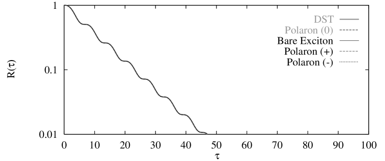
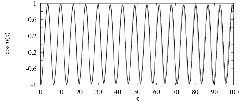
FIG. 1.: Time dependence of the total occupation (top) and of the relative site occupation difference (bottom) for $g=0.1$, $p=1$ and $r=10$. Different oscillator initial conditions for the full dynamic model and the DST dynamics can hardly be distinguished for this parameter set. They are shown in this and all the following figures with the line types indicated in the upper part. In the bottom plot, $\cos\theta=1$ corresponds to the sink site and $\cos\theta=-1$ to the sinkless site where the exciton is created. The lower/upper horizontal line shows the location of the fixed point B^- at the time of the creation of the exciton ($R=1$) and after its complete decay ($R=0$), respectively.

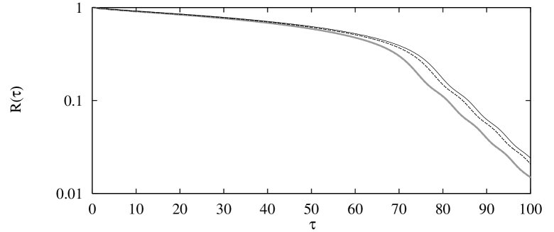
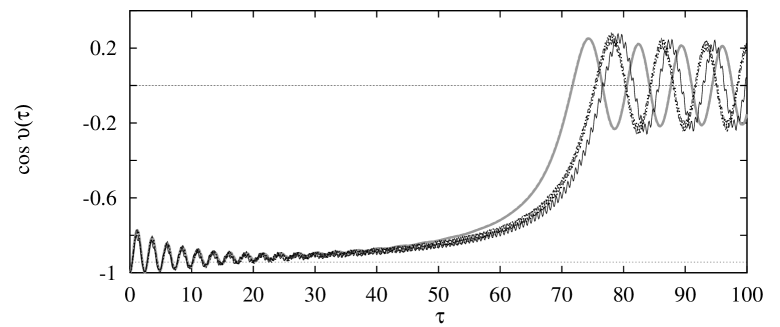
FIG. 2.: Time dependence of the total occupation (top) and of the relative site occupation difference (bottom) for $g=0.1$, $p=3$ and $r=10$.

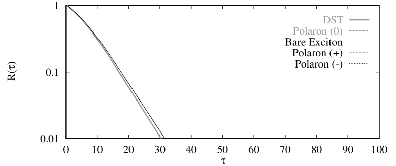
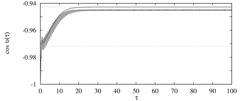
FIG. 3.: Time dependence of the total occupation (top) and of the relative site occupation difference (bottom - DST, bare exciton and polaron (0) only) for $g=3$, $p=3$ and $r=10$.

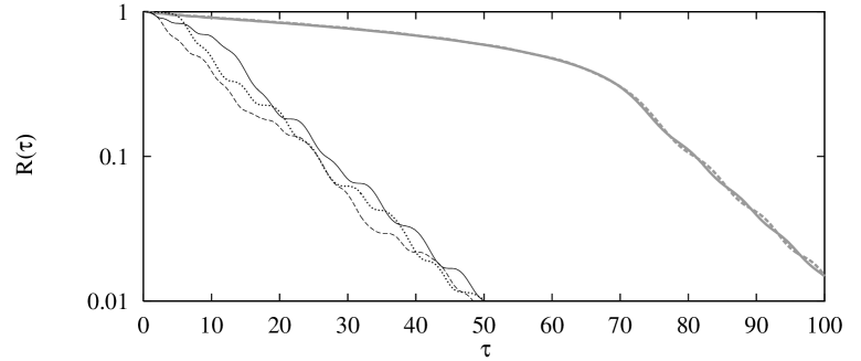
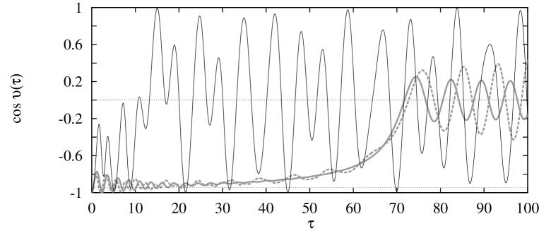
FIG. 4.: Time dependence of the total occupation (top) and of the relative site occupation difference (bottom - DST, bare exciton and polaron (0) only) for $g=0.1$, $p=3$ and $r=1$.

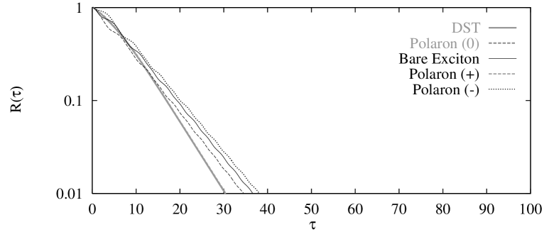
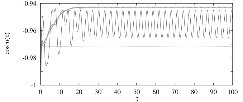
FIG. 5.: Time dependence of the total occupation (top) and of the relative site occupation difference (bottom - DST, bare exciton and polaron (0) only) for $g=3$, $p=3$ and $r=1$.

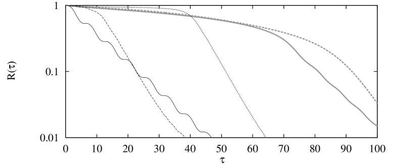
FIG. 6.: Time dependence of the total occupation for all initial conditions (top) and of the relative site occupation difference for the polaron (–) (bottom). With the sparse bold dots the time dependence of the two adiabatic states is indicated. The parameters are $g=0.1$, $p=3$ and $r=0.1$.

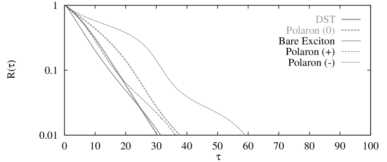
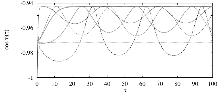
FIG. 7.: Time dependence of the total occupation (top) and of the relative site occupation difference (bottom) for $g=3$, $p=3$ and $r=0.1$. In the bottom plot for the polaron (–) solution beside the relative site occupation the time dependence of the lower adiabatic state is displayed with sparse bold dots.

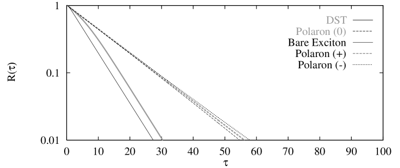
FIG. 8.: Time dependence of the total occupation for $g=3$, $p=3$ and $r=0.001$.

REFERENCES

- [1] H. Haken and P. Reineker. In A. B. Zahlan, editor, Excitons, magnons and phonons in molecular crystals. Cambridge University Press, Cambridge, 1968.
- [2] M. Grover and R. Silbey. J. Chem. Phys., 54:4843, 1970.
- [3] V. M. Kenkre, E. W. Montroll, and M. F. Shlesinger. J. Stat. Phys., 9:45–50, 1973.
- [4] R. Kühne and P. Reineker. Z. Phys. B, 22:201–206, 1975.
- [5] V. M. Kenkre. In G. Höhler, editor, Exciton Dynamics in Molecular Crystals and Aggregates, volume 94 of Springer Tracts in Modern Physics, pages 1–109. Springer, Berlin-Heidelberg-New York, 1982.
- [6] P. Reineker. In G. Höhler, editor, Exciton Dynamics in Molecular Crystals and Aggregates, volume 94 of Springer Tracts in Modern Physics 94, pages 111–226. Springer, Berlin-Heidelberg-New York, 1982.
- [7] A. Osuka, K. Marnyama, and I. Yamzaki. Chem. Phys. Lett., 165:392, 1990.
- [8] U. Rempel, B. von Maltzan, and C. von Borczyskowski. Chem. Phys. Lett., 169:347, 1990.
- [9] R. M. Pearlstein and H. Zuber. Antennas and Reaction Centers of Photosynthetic Bacteria, volume 42 of Springer Series in Chemical Physics. Springer, Berlin, 1985.
- [10] V. Čápek and V. Szöcs. phys. stat. sol. (b), 125:K137, 1984.
- [11] I. Barvík. In W. Gans, A. Blumen, and A. Aman, editors, Large Scale Molecular Systems, NATO ASI Series, pages 371–374. Plenum Press, New York, 1991.
- [12] I. Barvík. In A. Blumen, editor, Dynamical Processes in Condensed Molecular Systems, pages 275–287. World Scientific, Singapore, 1991.
- [13] I. Barvík and P. Heřman. phys. stat. sol. (b), 174:99–107, 1991. Czech. J. Phys., 41:1265–1280, 1991. Phys. Rev. B, 45:2772–2778, 1992.
- [14] P. Heřman and I. Barvík. Phys. Lett. A, 163:313–319, 1992. Phys. Rev. B, 48:3130–3139, 1993.
- [15] J. Appel. Solid State Physics, 21:193, 1968.
- [16] A. S. Davydov. Theory of Molecular Excitons. Plenum, New York, 1979.
- [17] M. Quack. Journal of Molecular Structure, 292:171, 1993.
- [18] J. C. Eilbeck, P. S. Lomdahl, and A. C. Scott. Physica D, 16:318–338, 1985.
- [19] V. M. Kenkre and D. K. Campbell. Phys. Rev. B, 34:4959–4961, 1986.
- [20] B. Esser and D. Hennig. Z. Phys. B, 83:285–293, 1991. Phys. Rev. A, 46:4569–4576, 1992.
- [21] M. Kus and V. M. Kenkre. Physica D, 79:409–415, 1994.
- [22] B. Esser and H. Schanz. Chaos, Solitons Fractals, 4:2067–2075, 1994. Z. Phys. B, 96:553–562, 1995.
- [23] H. Schanz and B. Esser. Z. Phys. B, 1996. accepted for publication.
- [24] V. M. Kenkre and H. L. Wu. Phys. Rev. B, 39:6907–6913, 1989.
- [25] D. Vitali, P. Allegrini, and P. Grigolini. Chem. Phys., 180:297, 1994.
- [26] V. Szöcs, P. Baňacký, and P. Reineker. Chem. Phys., 199:1–18, 1995.
- [27] I. Barvík, B. Esser, and H. Schanz. Phys. Rev. B, 52:9377–9386, 1995.
- [28] F. Verhulst. Nonlinear Differential Equations and Dynamical Systems. Springer, Berlin, 1990.