Theory of finite temperature crossovers near quantum critical points close to, or above, their upper-critical dimension

Abstract

A systematic method for the computation of finite temperature ($T$) crossover functions near quantum critical points close to, or above, their upper-critical dimension is devised. We describe the physics of the various regions in the $T$ and critical tuning parameter ($t$) plane. The quantum critical point is at $T=0$, $t=0$, and in many cases there is a line of finite temperature transitions at $T=T_{c}(t)$, $t<0$ with $T_{c}(0)=0$. For the relativistic, $n$-component $\phi^{4}$ continuum quantum field theory (which describes lattice quantum rotor ($n\geq 2$) and transverse field Ising ($n=1$) models) the upper critical dimension is $d=3$, and for $d<3$, $\epsilon=3-d$ is the control parameter over the entire phase diagram. In the region $|T-T_{c}(t)|\ll T_{c}(t)$, we obtain an $\epsilon$ expansion for coupling constants which then are input as arguments of known classical, tricritical, crossover functions. In the high $T$ region of the continuum theory, an expansion in integer powers of $\sqrt{\epsilon}$, modulo powers of $\ln\epsilon$, holds for all thermodynamic observables, static correlators, and dynamic properties at all Matsubara frequencies; for the imaginary part of correlators at real frequencies ($\omega$), the perturbative $\sqrt{\epsilon}$ expansion describes quantum relaxation at $\hbar\omega\sim k_{B}T$ or larger, but fails for $\hbar\omega\sim\sqrt{\epsilon}k_{B}T$ or smaller. An important principle, underlying the whole calculation, is the analyticity of all observables as functions of $t$ at $t=0$, for $T>0$; indeed, analytic continuation in $t$ is used to obtain results in a portion of the phase diagram. Our method also applies to a large class of other quantum critical points and their associated continuum quantum field theories.

I Introduction

The study of finite temperature crossovers in the vicinity of quantum phase transitions is a subject with a long history [1, 2, 3, 4, 5, 6, 7, 8, 9, 10, 11, 12, 13, 14, 15, 16, 17, 18, 19, 20, 21], but many aspects of it remain poorly understood. The structure of the crossovers is especially rich for the case where the quantum critical point extends into a line of finite temperature phase transitions, and there is a reasonable qualitative understanding of all the regimes. While there have been quantitative calculations of crossover functions in special cases [6, 9, 16, 18, 19, 20] there is no complete, general theory of these crossovers, especially for the case when the quantum critical point is below its upper critical dimension.

In this paper, we shall provide a new systematic and controlled approach to the quantitative computation of these crossover functions. Our method is quite general: it should apply to essentially all quantum critical points in the vicinity of, or above, their upper-critical dimension.

Recently, O’Connor and Stephens [22] have also studied crossovers near relativistic quantum-critical points below their upper-critical dimension. They found it necessary to introduce a non-standard extension of the field-theoretic renormalization group. We will comment on their results (and of others) in Section IV.

In this paper, we will show that it is possible to devise a simple strategy, completely with the framework of standard field-theoretic methods, which provides a systematic computation of the required crossovers. We shall describe how our method can be extended to arbitrary orders in an expansion in powers of the interactions, but we shall only provide here explicit computations at low orders. One of the main virtues of our method is that it clearly separates contributions of fluctuations of different physical origins: critical singularities of the $T=0$ quantum-critical point, and those of the finite $T$ classical phase transition, are accounted for at distinct stages of the calculation.

We shall present most of our discussion in the context of a continuum quantum field theory (CQFT) of a $n$-component bosonic field $\phi_{\alpha}$ ($\alpha=1\ldots n$; we will drop the index $\alpha$ except where needed) with $O(n)$ symmetry and with the bare, imaginary time ($\tau$) action

$${\cal S}=\int_{0}^{1/T}d\tau\int d^{d}x\left\{\frac{1}{2}\left[(\partial_{\tau}\phi)^{2}+(\nabla\phi)^{2}+(m_{0c}^{2}+t_{0})\phi^{2}\right]+\frac{u_{0}}{4!}\phi^{4}\right\}.$$ (1)

We have set $\hbar=k_{B}=1$, measured length scales ($x$) in units in which the velocity of excitations $c=1$, and introduced the bare mass $m_{oc}^{2}+t_{0}$ and the bare coupling $u_{0}$ (the mass term has been separated so that the $T=0$ quantum critical point is at $t_{0}=0$). This field theory describes the low-energy physics in the vicinity of the quantum phase transition in the $d$-dimensional transverse-field Ising model (for $n=1$) or the $O(n)$ quantum rotor model (for $n>1$). The generalization of our method to other quantum field theories, like the dilute Bose gas, or the models for onset of antiferromagnetism in Fermi liquids, is straightforward and will also be discussed.

We begin our discussion by reviewing the expecting scaling structure of ${\cal S}$ for the case where the quantum critical point is below its upper critical dimension. At $T=0$, ${\cal S}$ describes the usual $\phi^{4}$ theory in $d+1$ dimensions, and its upper critical dimension is $d=3$; for $d<3$, there is an essentially complete understanding [23, 24] of the critical properties of this theory in an expansion in powers of

$$\epsilon=3-d.$$ (2)

The definition of the renormalized theory requires a field scale renormalization $Z$, a coupling constant renormalization $Z_{4}$, and a renormalization of $\phi^{2}$ insertions in the critical theory $Z_{2}$. In terms of these, we define us usual

$$t=t_{0}Z/Z_{2};$$ (3)

$t$ is a measure of the deviation of the system from its $T=0$ quantum critical point. Precisely the same renormalizations are also sufficient to define a finite theory at non-zero $T$, even in the vicinity of the finite $T$ phase transition line, as we shall explicitly see in this paper.

We show a sketch of the phase diagram of ${\cal S}$ as a function of $t$ and $T$ in Fig 1 [21]. We have assumed in this figure, and throughout the remainder of the paper that the model ${\cal S}$ is in its scaling limit i.e. the coupling $u_{0}$ is at its fixed point value, and all ultraviolet cutoffs have been sent to infinity after an appropriate renormalization procedure. There is a finite temperature phase transition line at $T=T_{c}(t)$, and all other boundaries are smooth crossovers. All of the physics is contained within universal quantum-critical crossover functions, which we now briefly describe. We will consider the behavior of the dynamic two-point susceptibility, $\chi(k,\omega)$ ($k$ is a spatial momentum, and $\omega$ is a frequency) obtained after analytic continuation of the susceptibility

$$\chi(k,i\omega_{n})=\frac{1}{Z}\int d^{d}x\int_{0}^{1/T}d\tau e^{i(kx-\omega_{n}\tau)}\langle\phi(x,\tau)\phi(0,0)\rangle$$ (4)

which is evaluated at Matsubara frequency $\omega_{n}=2n\pi T$. We will consider the scaling behavior of $\chi$ for $t>0$ and $t<0$ separately, and then discuss the relationship between the two cases.

(i) $t>0$: The susceptibility $\chi$ obeys the scaling form [9]

$$\chi(k,\omega)={\cal A}\left(\frac{\hbar c}{k_{B}T}\right)^{2}\left(\frac{k_{B}T}{\Delta_{+}}\right)^{\eta}\Psi_{+}\left(\frac{\hbar ck}{k_{B}T},\frac{\hbar\omega}{k_{B}T},\frac{\Delta_{+}}{k_{B}T}\right)~{}~{}~{}~{}~{}~{}~{}~{}t>0$$ (5)

where we have momentarily re-inserted all factors of $\hbar$, $k_{B}$, and $c$, $\eta$ is the usual field anomalous dimension of the $T=0$, $d+1$ dimensional theory, and $\Psi_{+}$ is a fully universal, complex-valued, universal scaling function. Notice that there are no arbitrary scale factors, and $\chi$ is fully determined by two parameters, $\Delta_{+}$ and ${\cal A}$, which are properties of the $T=0$ theory. The first of these, $\Delta_{+}$, is the true energy gap above the ground state, while the second, ${\cal A}$, is the residue of the lowest quasi-particle excitation; they obey

$${\Delta}_{+}\sim t^{\nu}~{}~{}~{}~{};~{}~{}~{}~{}{\cal A}\sim t^{\eta\nu}~{}~{}~{}~{}~{}~{}~{}~{}~{}~{}t>0$$ (6)

where $\nu$ is the usual correlation length exponent of the $T=0$ theory (all Greek letter exponents in this paper refer to those of $T=0$ the quantum-critical point, and not to those the finite $T$ phase transition). We provide a computation of the values of the $T=0$ parameters, $\Delta_{+}$ and ${\cal A}_{+}$, in Appendix B.

The factors in front of $\Psi_{+}$ in (5) have been chosen so that $\Psi_{+}$ is finite at $\Delta_{+}/k_{B}T=0$. All scaling functions defined in this paper will share this property.

We also emphasize that although the scaling ansatz (5) contains dynamic information, its form and content are quite different from the dynamic scaling hypotheses applied near classical phase transitions [25]. In these classical systems, a single diverging correlation length, $\xi$, is used to set the scale for $k$ and $\omega$; the analog of (5) is then a scaling function of two arguments, $k\xi$ and $\omega\xi^{z_{c}}$, where $z_{c}$ is the classical dynamic critical exponent. In contrast, the quantum crossover result (5) is a function of three arguments, the extra argument arising because the quantum critical point has two relevant perturbations ($T$ and $t$). Further, the identification of universal scale factors, and indeed the conceptualization of the physics, is much more transparent when $T$ is used as the primary energy setting the scale for other perturbations. Only in the immediate vicnity of the finite $T$ phase transition at $T_{c}(t)$, $|T-T_{c}(t)|\ll T_{c}(t)$, does (5) collapse into a scaling function of two arguments, as has been discussed in Refs [9, 26].

(ii) $t<0$: Now the $T=0$ ground state breaks a symmetry with

$$\langle\phi_{\alpha}\rangle=N_{0}\delta_{\alpha 1}~{}~{}~{}~{}~{}~{}~{}~{}T=0,t<0;$$ (7)

here $N_{0}\sim(-t)^{\beta}$ is the condensate, which we have arbitrarily chosen to point in the $\alpha=1$ direction, and $\beta=(d-1+\eta)\nu/2$ is the magnetization exponent of the $T=0$ theory. Now $N_{0}$ can serve as the parameter which determined the field scale (replacing ${\cal A}$), and we need an energy scale which determines the deviation of the ground state from the $t=0$, $T=0$ quantum critical point. For $n=1$, there is a gap, $\Delta_{-}$, above the ground state, which satisfies our requirements; we have therefore [9]

$$\chi(k,\omega)=\frac{N_{0}^{2}(\hbar c)^{d}}{\Delta_{-}^{d-1+\eta}(k_{B}T)^{2-\eta}}\Psi_{-}\left(\frac{\hbar ck}{k_{B}T},\frac{\hbar\omega}{k_{B}T},\frac{\Delta_{-}}{k_{B}T}\right)~{}~{}~{}~{}~{}~{}~{}t<0,n=1.$$ (8)

For $n\geq 2$, there is no gap above the ground state, and we use instead the spin-stiffness, $\rho_{s}\sim(-t)^{(d-1)\nu}$ as a measure of the deviation from the quantum critical point; in this case we have the scaling form

$$\chi_{\alpha}(k,\omega)=\frac{N_{0}^{2}}{\rho_{s}}\left(\frac{\hbar c}{k_{B}T}\right)^{2}\left(\frac{(k_{B}T)^{d-1}}{(\hbar c)^{d-2}\rho_{s}}\right)^{\eta/(d-1)}\Psi_{-\alpha}\left(\frac{\hbar ck}{k_{B}T},\frac{\hbar\omega}{k_{B}T},\frac{(\hbar c)^{d-2}\rho_{s}}{(k_{B}T)^{d-1}}\right)~{}~{}~{}~{}~{}t<0,n\geq 2.$$ (9)

A computation of the $T=0$ parameters $N_{0}$, $\Delta_{-}$ and $\rho_{s}$ is provided in Appendix B. The $\alpha$ dependence in (9) accounts for the difference between fluctuations transverse and longitudinal to the condensate orientation. Again, $\Psi_{-}$ is finite at $\Delta_{-}/k_{B}T=0$, or at $\rho_{s}/T^{d-1}=0$, and all subsequent scaling functions will share this property. The finite temperature phase transition at $T_{c}(t)$ is contained entirely within the scaling function $\Psi_{-}$: this transition appears as a point of non-analyticity of $\Psi_{-}$ as a function of $\Delta_{-}/T$ or $\rho_{s}/T^{d-1}$. An immediate consequence is that the value of $T_{c}$ can be determined precisely in terms of the $T=0$ energy scale; we found, in an expansion in powers of $\epsilon$, that

$$T_{c}=\frac{\Delta_{-}}{k_{B}\sqrt{\epsilon}}\left[\frac{3}{2\pi}+{\cal O}(\epsilon,\epsilon^{(1+\epsilon)/(1-\epsilon)},\epsilon^{1/(2\nu)})\right]~{}~{}~{}~{}~{}~{}n=1$$ (10)

and

$$T_{c}=\frac{(\hbar c)^{(d-2)/(d-1)}\rho_{s}^{1/(d-1)}}{k_{B}}\left[\left(\frac{3}{2\pi^{2}(n+2)}\right)^{1/2}+{\cal O}(\epsilon,\epsilon^{(1+\epsilon)/(1-\epsilon)},\epsilon^{1/(2\nu)})\right]~{}~{}~{}~{}~{}~{}n\geq 2$$ (11)

The various higher order contributions are all universal, but arise from very different physical effects; we will discuss their origin later in the paper. In the upper critical dimension ($\epsilon=0$), these formulae are modified by replacing $\epsilon$ by $1/\ln$’s : so for $n=1$, $T_{c}\sim\Delta_{-}\ln^{1/2}(1/\Delta_{-})$ etc. For the cases $n=1$, $d=1$ and $n\geq 3$, $d=2$ it is known that in fact $T_{c}=0$ i.e. long-range order is present only at $T=0$, and disappears at any non-zero $T$. For these cases, it is clear that the above results for $T_{c}$, and other results obtained in the $\epsilon$ expansion, cannot be used in the region labeled III in Fig 1. However, the results of this paper can still be usefully applied to the remainder of the phase diagram of Fig 1.

Although we have used two separate scaling forms to describe the behavior for $t<0$ and $t>0$, there is a crucial connection between them. Notice that there is no thermodynamic singularity at $t=0$ provided $T>0$. This implies that the observable $\chi(k,\omega)$ (and indeed all other observables) must be analytic as a function of $t$ at $t=0$ as long as $T>0$. This principle will serve as an extremely important constraint on the calculation in this paper; indeed, our method is designed to ensure that analyticity holds at each order. Further, our results in the region $t<0$, $T>T_{c}(t)$, were obtained by a process of analytic continuation from the $t>0$, $T>0$ region (see Fig 1). The ground state for $t<0$ has a spontaneously broken symmetry, and hence cannot be used to access the symmetric $t<0$, $T>T_{c}(t)$ region in perturbation theory; instead it is more naturally accessed from the disordered side with $t>0$. A similar procedure of analytic continuation in coupling constant was used recently in exact determinations of quantum critical scaling functions in $d=1$ [26].

Before turning to a description of our method in Section I A, we highlight one of our new results. A particularly interesting property of CQFT’s at finite $T$ is the expected thermal relaxational behavior of their correlators in real time. This behavior cannot be characterized simply to a field-theorist who merely considers correlators of ${\cal S}$, defined as a CQFT in imaginary time with a spacetime geometry $R^{d}\times S_{1}$ (the tensor product of infinite $d$-dimensional flat space with a circle of circumference $1/T$). In real frequency, the thermal relaxational behavior is characterized by the fact that $\lim_{\omega\rightarrow 0}\mbox{Im}\chi(k,\omega)/\omega$ is expected to be finite, with the limiting value proportional to a relaxation constant. In Ref [21], the quantity

$$\Gamma_{R}^{-1}\equiv i\chi(0,0)\left.\frac{\partial\chi^{-1}(0,\omega)}{\partial\omega}\right|_{\omega=0}$$ (12)

was introduced as a convenient characterization of the relaxation rate. By (5), $\Gamma_{R}$ must obey a scaling form given by

$$\Gamma_{R}=\frac{k_{B}T}{\hbar}\Psi_{\Gamma+}\left(\frac{\Delta_{+}}{k_{B}T}\right),$$ (13)

for $t>0$, and similarly for $t<0$. In particular, in the high $T$ limit of the CQFT [21] (this is region II of Fig 1), $\Gamma_{R}$ is $(k_{B}T/\hbar)$ times $\Psi_{\Gamma+}(0)$, which is expected to be a finite, universal number. Unfortunately, we shall find that the perturbative expansion discussed in this paper cannot be used to obtain a systematic expansion for $\Gamma_{R}$. A self-consistent approach, with damping of intermediate states, appears necessary and will not be discussed here. In the high $T$ limit, we shall show that the non-self-consistent approach fails for frequencies of order $\sqrt{\epsilon}T/\hbar$ or smaller. To avoid this difficulty, let us define an alternative characterization of the damping at frequencies of order $k_{B}T/\hbar$ by

$$\Gamma_{RT}^{-1}\equiv-\chi(0,0)\left.\mbox{Im}\frac{\chi^{-1}(0,\omega)}{\omega}\right|_{\omega=k_{B}T/\hbar}$$ (14)

This will obey a scaling form identical to that of $\Gamma_{R}$. We found in the high $T$ limit that

$$\frac{k_{B}T}{\hbar\Gamma_{RT}}=\epsilon\frac{3}{(n+8)\pi}\left[\frac{1}{8}+\pi^{2}+6\mbox{Li}_{2}(e^{-1/2})\right]+{\cal O}(\epsilon^{3/2}),$$ (15)

where $\mbox{Li}_{2}$ is the dilogarithm function defined in (85). The result will be compared with an exact result for $\Gamma_{RT}$ for $d=1$, $n=1$ in Section II B. Also in the exact result at $d=1$, $n=1$ we find $\Gamma_{RT}/\Gamma_{T}=0.98170018\ldots$ in the high $T$ limit, and we expect a similar ratio close to unity in all cases in region II of Fig 1.

The following subsection contains a description of our approach. Readers not interested in the details of its application to ${\cal S}$, can read Section I A, and skip ahead to Section IV where we give our unified perspective of this and earlier work.

We will revert to setting $\hbar=k_{B}=c=1$ in the remainder of the paper.

A The Method

The origin of the approach we shall take here can be traced to early work by Luscher [27] on the quantum $O(n)$ non-linear sigma model in $1+1$ dimensions. Subsequently, a related idea was employed by Brezin and Zinn-Justin [28] and by Rudnick, Guo and Jasnow [29] in their study of finite-size scaling crossover functions in systems which are finite in all, or all but one, dimensions (also referred to as the $d\rightarrow 0$ and $d\rightarrow 1$ crossovers). The quantum-critical crossovers are clearly related, but now involve $d+1\rightarrow d$. We shall show here that the latter problem can be successfully analyzed by essentially the same method as that used for the former. There are some new subtleties that arise in a limited region of the phase diagram, and we will discuss below how they can be dealt with.

We will describe the method here for the special case of the action ${\cal S}$ (Eqn (1)) with $d$ below its upper critical dimension i.e. $d<3$. The central idea is that at finite $T$, it is safe to integrate out all modes of $\phi(k,\omega_{n})$ with a non-zero Matsubara frequency, $\omega_{n}\neq 0$, to derive an effective action for zero frequency modes $\phi(k,\omega_{n}=0)$. All modes being integrated out are regulated in the infrared by the $\omega_{n}^{2}$ term in their propagator, and so the process is necessarily free of infrared divergences; further, the renormalizations of the $T=0$ theory also control the ultraviolet divergences at finite $T$. To be specific, let us define

$$\Phi(x)\equiv\frac{T}{\sqrt{Z}}\int_{0}^{1/T}d\tau\phi(x,\tau),$$ (16)

and its transform in momentum space $\Phi(k)=\int d^{d}xe^{ikx}\Phi(x)$. Then from ${\cal S}$, we can deduce an effective action for $\Phi(k)$ after completely integrating out the $\phi(k,\omega_{n}\neq 0)$ (we have set the coupling $u_{0}$ at the fixed-point of its $\beta$-function—see Appendix B):

$${\cal S}_{eff}=\frac{1}{T}\left[\frac{1}{2}\int\frac{d^{d}k}{(2\pi)^{d}}\widetilde{C}_{2}(k)|\Phi(k)|^{2}\right.$$ (17)

$$+\left.\frac{1}{4!}\int\frac{d^{d}k_{1}d^{d}k_{2}d^{d}k_{3}}{(2\pi)^{3d}}\widetilde{C}_{4}(k_{1},k_{2},k_{3},-k_{1}-k_{2}-k_{3})\Phi(k_{1})\Phi(k_{2})\Phi(k_{3})\Phi(-k_{1}-k_{2}-k_{3})+\ldots\right].$$ (18)

The couplings $\widetilde{C}_{2}$, $\widetilde{C}_{4}$, $\ldots$, are computed in a power series in $\epsilon$, with the coupling constants renormalized as in the $T=0$, $d+1$ dimensional critical theory. This procedure will remove all the ultraviolet divergences of the quantum critical point. However, the ultraviolet divergences of the finite $T$, $d$-dimensional $\phi^{4}$ theory remain; fortunately these are very simple as the $\phi^{4}$ theory is super-renormalizable for $d<4$ [30]. In particular, $d<3$, ultraviolet divergences are associated only with the one-loop ‘tadpole’ graphs; so let us define

$$C_{2}(k)=\widetilde{C}_{2}(k)+\left(\frac{n+2}{6}\right)\int\frac{d^{d}k_{1}}{(2\pi)^{d}}\frac{\widetilde{C}_{4}(k,-k,k_{1},-k_{1})}{k_{1}^{2}}+\ldots$$ (19)

where the ellipses refer to “tadpole” contributions from higher order vertices like $\widetilde{C}_{6}$, $\widetilde{C}_{8}$ $\ldots$. Similarly, there will also be tadpole renormalizations of $\widetilde{C}_{4}$ to $C_{4}$ by higher order vertices, and so on. These new vertices, $C_{2p}$, $p$ integer, are now free of all ultraviolet divergences (for $3\leq d<4$ there is a second classical renormalization at the two-loop level which must be accounted for; we will ignore this complication here and deal with it later in the paper). They are also automatically free of infrared divergences as we are only integrating out modes with a finite frequency. Indeed, these vertices must obey the scaling forms:

$$C_{2p}(k_{i})=T^{d+1-p(d-1+\eta)}\left(\frac{\Delta_{+}^{\eta}}{{\cal A}}\right)^{p}\Psi_{Q+}^{(p)}\left(\frac{k_{i}}{T},\frac{\Delta_{+}}{T}\right),$$ (20)

for $t>0$, with the $\Psi_{Q+}^{(p)}$ a set of quantum scaling functions; the subscript $Q$ emphasizes that these scaling functions are properties of the $T=0$ quantum-critical point, and distinguishes them from classical crossover functions we shall use later. Similar scaling results hold for $t<0$ and we will refrain from explicitly displaying them. For our subsequent discussion it is useful to define a set of couplings $K$, $R$, and $U$, which can be obtained from the $C_{2p}$, and which play an important role in our analysis:

$$R \equiv C_{2}(0)$$ (21)

$$K \equiv \left(1+\left.\frac{\partial C_{2}(k)}{\partial k^{2}}\right|_{k=0}\right)$$ (22)

$$U \equiv C_{4}(k_{i}=0)$$ (23)

It is clear that $R$, $K$, and $U$ obey scaling forms that can be easily deduced from (20).

We also note that the couplings $R$ and $C_{2p}(k_{i})$ are guaranteed to be analytic as a function of $t$ at $t=0$; this is because only finite frequency modes have been integrated out, and their propagator $1/(k^{2}+\omega_{n}^{2}+t)$ is not singular at $t=0$ in the infrared ($k=0$) as $\omega_{n}\neq 0$. This analyticity will be of great use to us later.

Assume, for the rest of this section, that we know the $\Psi_{Q\pm}^{(p)}$ functions (we will provide explicit computations of some of them later in the paper). We are now faced with the seemingly difficult problem of computing observables in the $\Phi$ theory with the action ${\cal S}_{eff}$. This is a theory in dimension $d$ close to 3 (not $d$ close to 4), and one might naively assume, that this problem is intractable. We shall now argue that, in fact, it is not. The argument is contained in the following two simple, but important, observations.
(1) Consider a perturbation theory of ${\cal S}_{eff}$ in which the propagator is $1/(Kk^{2}+R)$, and we expand in the non-linearities $C_{2p}(k_{i})$, $p\geq 2$ in powers of $\epsilon$. This expansion differs from an ordinary expansion in powers of $\epsilon$ only in that the mass $R$ and coupling $K$ itself contain corrections in powers of $\epsilon$; alternatively one could also treat $K-1$ as an interaction, and work with the propagator $1/(k^{2}+R)$, but it is essential to keep the mass $R$ in the propagator. Such a procedure is guaranteed to be finite in the ultraviolet. This follows immediately from the statement that the renormalization of the $T=0$ theory (which we carried out while obtaining ${\cal S}_{eff}$ from ${\cal S}$) is sufficient to remove ultraviolet divergences even at non-zero $T$. In other words, the momentum dependencies in the $C_{2p}(k_{i})$ must be such that all ultraviolet divergences cancel out.
(2) The action ${\cal S}_{eff}$ is weakly coupled over the bulk of the phase diagram in the $t,T$ plane, and so the procedure in (1) leads to accurate results for physical observables. Only in the region $|T-T_{c}(t)|\ll T_{c}(t)$ (drawn shaded in Fig 1) is a more sophisticated analysis necessary, which will be described momentarily. To verify this claim, consider the values of the low order couplings in ${\cal S}_{eff}$ at $t=0$, but $T$ finite; we will find later that

$$R \sim \epsilon T^{2-\eta}$$ (24)

$$K \sim T^{-\eta}$$ (25)

$$U \sim \epsilon T^{\epsilon-2\eta}$$ (26)

for $t=0$. (For the present purpose, we can neglect all $C_{2p}$ for $p>2$ as they are all of order $\epsilon^{2}$.) A dimensionless measure of the strength of non-linearities in ${\cal S}_{eff}$ is

$$\frac{TU}{K^{d/2}R^{(4-d)/2}}\sim\epsilon^{(1-\epsilon)/2}\sim\sqrt{\epsilon}\left(1-\frac{\epsilon\ln\epsilon}{2}\right)\ll 1~{}~{}~{}~{}~{}~{}~{}~{}\mbox{for $t=0$}.$$ (27)

The above dimensionless ratio is simply that appearing in the familiar Ginzburg criterion [31]. So a simple perturbative calculation is adequate for $t=0$. For $t>0$, the behavior of perturbation theory can only improve as the mass $R$ becomes larger, which decreases the value of the above dimensionless ratio; as a result the perturbative calculation describes the crossover between the quantum-critical and quantum-disordered regimes of Fig 1. For $t<0$ the perturbation theory is initially adequate, but eventually becomes unreliable in the region $|T-T_{c}(t)|\ll T_{c}(t)$.

As the above results contain some the key points which allowed the computations of this paper, it is useful to reiterate them. We describe the nature of our expansion, excluding the shaded region $|T-T_{c}(t)|\ll T_{c}(t)$ of Fig 1. The first step is to obtain an expansion for the ‘mass’ $R$ of the $\omega_{n}=0$ mode: we outlined above a procedure which yields a series in integer powers of $\epsilon$. Then, generate an expansion for the physical observable of interest, temporarily treating $R$ as a fixed constant independent of $\epsilon$; this will again be a series in integer powers of $\epsilon$, but strong infrared fluctuations of the $\omega_{n}=0$ mode lead to a singular dependence of the latter series on $R$. Finally, insert the former series for $R$ into the latter series for the physical observable. In the quantum-disordered region (Fig 1), $R$ is of order unity, and the final result remains a series in integer powers of $\epsilon$. However, in the quantum-critical region, $R$ is of order $\epsilon$ (Eqn (26)) and the result, by (27), is a series in integer powers of $\sqrt{\epsilon}$, with possibly a finite number of powers of $\ln\epsilon$ multiplying the terms. It is important to note that the final series in powers of $\sqrt{\epsilon}$ is obtained from the original series in powers of $\epsilon$ only by a local re-arrangement of terms i.e. given all the terms up to a certain order in the $\epsilon$ series, we can obtain all terms below a related order in the $\sqrt{\epsilon}$ series.

Finally, let us turn our attention to the troublesome region $|T-T_{c}(t)|\ll T_{c}(t)$. We expect this region to be dominated by the classical fluctuations characteristic of the finite temperature transition, and hence to be well described by the following action ${\cal S}_{C}$, which is a truncated form of ${\cal S}_{eff}$:

$${\cal S}_{C}=\frac{1}{T}\int d^{d}x\left[\frac{K}{2}(\nabla{\Phi})^{2}+\frac{R}{2}{\Phi}^{2}+\frac{U}{4!}{\Phi}^{4}\right].$$ (28)

The couplings above were defined in (23). We have implicitly performed tadpole renormalizations where necessary to remove ultraviolet divergences of the classical theory. An immediate consequence of the super-renormalizability of the classical ${\cal S}_{C}$ is that all observables are universal functions of the “bare” coupling constants $K$, $R$ and $U$. So for example, we have for the static susceptibility

$$\chi(k,i\omega_{n}=0)=\frac{1}{T}\langle|\Phi(k)|^{2}\rangle=\frac{1}{R}\Psi_{C}\left(\frac{Kk^{2}}{R},\frac{TU}{K^{d/2}R^{(4-d)/2}}\right)$$ (29)

where $\Psi_{C}$ is a universal crossover function with no arbitrary scale factors. In fact, the crossover function $\Psi_{C}$ has been considered earlier in Ref [32], where it was dubbed the tricritical crossover function for entirely different physical reasons (we emphasize that this terminology is purely accidental - we are not dealing with any tricritical point here). The computation of tricritical crossover functions is a logically separate problem from those considered in this paper, and we shall have relatively little to say about them here. We shall simply treat them as known, previously computed functions; for completeness, we tabulate some results on these functions in Appendix A. Notice that the arguments of the classical crossover function $\Psi_{C}$ in (29) are themselves quantum-critical crossover functions, as follows from (20) and (23). Indeed, inserting (20) and (23) into (29), we get a scaling form completely consistent with (5). The critical temperature, $T_{c}$, is determined by the condition $\chi(0,0)=\infty$; in general, this is not equivalent to the requirement $R=0$ (although this does turn out to be the case at the one-loop level), but is instead given by the point where the scaling function $\Psi_{C}$ diverges. This condition leads to equation $TU/(K^{d/2}R^{(4-d)/2})=\mbox{constant}$ where the constant is determined by the point where $\Psi_{C}$ diverges as a function of its second argument; it is the solution of this equation which leads to the ${\cal O}(\epsilon^{(1+\epsilon)/(1-\epsilon)})$ corrections to the result for $T_{c}$ reported in (10).

To summarize, in the region $|T-T_{c}(t)|\ll T_{c}(t)$, the physics is described by universal crossover functions, $\Psi$, which are “crossover functions ($\Psi_{C}$) of crossover functions ($\Psi_{Q}$)”. The $\Psi_{Q}$ functions are properties of the quantum-critical point, and it is the burden of this paper to compute them; these functions then serve as arguments of known classical, tricritical crossover functions ($\Psi_{C}$).

Finally, we note that for $d$ just below 3, it is also necessary to include a coupling $V\Phi^{6}$ in ${\cal S}$ to get the correct infrared behavior; we have ignored this complication for simplicity; moreover, as $V\sim\epsilon^{3}$ and this effect is present only at a rather high order.

The outline of the remainder of the paper is as follows. In Section II we will compute properties of ${\cal S}$ for $d<3$. The discussion is divided into a one-loop computation of static observables in Section II A and a two loop computation of dynamic observables in Section II B. Section III will present a general discussion of the properties of models above their upper critical dimension: the modifications necessary in the scaling forms and the explicit computation of crossover functions. Finally Section IV will review the main results, discuss their relationship to previous works, and point out directions for future work. A number of details of the calculations appear in the appendices. The tricritical crossover functions appearing in (29) are in Appendix A. In Appendix B we compute the $T=0$ parameters that appear in the scaling forms. Details of the finite $T$ two-loop computations of various quantities are in Appendix C.

II Crossover functions of ${\cal S}$ below three dimensions

A number of crossover functions for the model ${\cal S}$ were introduced in Section I. We give formal expressions, valid to two-loop order, for all of these quantities in Appendix C. In this section we will evaluate these expressions and show that they obey the required scaling forms order-by-order in $\epsilon$. We will discuss the behavior for general values of $t$ only to one-loop order in Section II A. We will limit our explicit two-loop results to a few important quantities at the critical coupling $t=0$; these will appear in Section II B.

The same basic trick will be repeatedly used to evaluate the frequency summations in Appendix C: we will always subtract from the summation of a function of $\omega_{n}$, the integration over frequency of precisely the same function. The resulting difference will always turn out to be strongly convergent as a function of momentum in all $d$. So, for example, we have:

$$T\sum_{\epsilon_{n}}\int\frac{d^{d}q}{(2\pi)^{d}}\frac{1}{\epsilon_{n}^{2}+q^{2}+a^{2}}- \int\frac{d\epsilon}{2\pi}\int\frac{d^{d}q}{(2\pi)^{d}}\frac{1}{\epsilon^{2}+q^{2}+a^{2}}$$ (32)

$$=T\sum_{\epsilon_{n}}\int\frac{d^{d}q}{(2\pi)^{d}}\frac{1}{\epsilon_{n}^{2}+q^{2}+a^{2}}-\int\frac{d^{d+1}p}{(2\pi)^{d}}\frac{1}{p^{2}+a^{2}}$$

$$=\int\frac{d^{d}q}{(2\pi)^{d}}\frac{1}{\sqrt{q^{2}+a^{2}}}\frac{1}{e^{\sqrt{q^{2}+a^{2}}/T}-1}$$

Notice that the integrand on the right hand side of the last equation falls off exponentially for large $q$, and the integral is therefore convergent for all $d$.

A One loop results

We will begin (Section II A 1) by determining the coupling constants $R$, $K$ and $U$ of ${\cal S}_{cl}$ which are the arguments of the tricritical crossover functions. Subsequently, we will present results for observables of ${\cal S}$: the susceptibility $\chi$ (Section II A 2) and the response of the system to a field that couples to the conserved $O(n)$ charge (Section II A 3).

1 Coupling constants of ${\cal S}_{cl}$

We begin by using (C18) and (23) to obtain an expression for $R$, valid to one-loop order:

$$R=t_{0}+u_{0}\left(\frac{n+2}{6}\right)\left[\int\frac{d^{d}q}{(2\pi)^{d}}\left(T\sum_{\epsilon_{n}\neq 0}\frac{1}{\epsilon_{n}^{2}+q^{2}+t_{0}}+\frac{T}{q^{2}}\right)-\int\frac{d^{d+1}p}{(2\pi)^{d+1}}\frac{1}{p^{2}}\right]$$ (33)

We have set $Z=1$ at this order, and will implicitly do so in the remainder of this section. We now apply the identity (32), perform the momentum integrals over $p$, express in terms of the renormalized $t$ using (3). Finally we express $u_{0}$ is terms of a renormalized coupling $g$ defined by

$$g=\mu^{-\epsilon}S_{d+1}\frac{Z^{2}}{Z_{4}}u_{0},$$ (34)

where $\mu$ is a renormalization momentum scale, $S_{d}=2/(\Gamma(d/2)(4\pi)^{d/2})$ is a phase space factor, and the values of the renormalization constants are tabulated in (B3). This gives for $t>0$:

$$R= t\left(1+\frac{n+2}{6\epsilon}g\right)+\mu^{\epsilon}g\left(\frac{n+2}{12}\right)\Gamma\left(2-\frac{\epsilon}{2}\right)\Gamma\left(-1+\frac{\epsilon}{2}\right)t^{1-\epsilon/2}$$ (36)

$$~{}~{}~{}~{}~{}~{}~{}~{}~{}~{}~{}~{}~{}~{}~{}~{}~{}~{}~{}~{}~{}~{}~{}~{}~{}~{}~{}~{}~{}~{}+g\left(\frac{n+2}{6}\right)T^{2}\left(\frac{\mu}{T}\right)^{\epsilon}F_{d}\left(\frac{t}{T^{2}}\right)$$

$$= t\left(1+\epsilon\frac{n+2}{2(n+8)}\ln\frac{t}{\mu^{2}}\right)+\epsilon T^{2}\left(\frac{n+2}{n+8}\right)F_{3}\left(\frac{t}{T^{2}}\right).$$ (37)

In the second equation, we have evaluated at the fixed point value $g=g^{\ast}$ (Eqn (B4)), and then expanded to order $\epsilon$. The function $F_{d}$ is given by

$$F_{d}(y)=\frac{1}{S_{d+1}}\int\frac{d^{d}k}{(2\pi)^{d}}\left[\frac{1}{\sqrt{k^{2}+y}}\frac{1}{e^{\sqrt{k^{2}+y}}-1}-\frac{1}{k^{2}+y}+\frac{1}{k^{2}}\right].$$ (38)

Let us also note here the values

$$F_{d}(0)=\frac{(4\pi)^{1/2}\Gamma((d+1)/2)\Gamma(d-1)\zeta(d-1)}{\Gamma(d/2)}~{}~{}~{}~{}~{}~{},~{}~{}~{}~{}~{}~{}F_{3}(0)=\frac{2\pi^{2}}{3}$$ (39)

It is now easy to see, using (B8) that the result (37) for $R$ can be written in the scaling form

$$R=\frac{T^{2-\eta}\Delta_{+}^{\eta}}{{\cal A}}\left(\frac{\Delta_{+}^{2}}{T^{2}}+\epsilon\left(\frac{n+2}{n+8}\right)F_{3}\left(\frac{\Delta_{+}^{2}}{T^{2}}\right)\right).$$ (40)

This result is consistent with the scaling postulated in (20). At this order, the exponent $\eta=0$, and verifying the powers of $\eta$ in front requires a higher order computation.

We now wish to extend this result for $R$ to $t<0$ by analytic continuation from the $t>0$ result. First, we need to verify that the $t>0$ result for $R$ is analytic at $t=0$. To do this, we first rewrite (37) in the form

$$R=t\left(1+\epsilon\frac{n+2}{n+8}\ln\frac{T}{\mu}\right)+\epsilon T^{2}\frac{n+2}{n+8}G_{+}\left(\frac{t}{T^{2}}\right)$$ (41)

where

$$G_{+}(y)=\frac{y\ln y}{2}+4\int_{0}^{\infty}k^{2}dk\frac{1}{\sqrt{k^{2}+y}}\frac{1}{e^{\sqrt{k^{2}+y}}-1}+2\pi\sqrt{y}$$ (42)

The first term in (41) is clearly a smooth function of $t$; if we can now show that $G_{+}(y)$ is a smooth function of $y$ near $y=0$, we will have established the analyticity of $R$ at $t=0$. Performing an integration by parts of the integral in (42), followed by an elementary re-arrangement of terms, we can manipulate the result for $G_{+}(y)$ into the following form:

$$G_{+}(y)= \frac{y\ln y}{2}+2\pi\sqrt{y}-4\int_{0}^{\infty}dk\ln\left[1-e^{-\sqrt{k^{2}+y}}\right]$$ (43)

$$= \frac{y\ln y}{2}+2\pi\sqrt{y}+2\int_{0}^{\infty}dk\left(\sqrt{k^{2}+y}-k-\ln\left[\frac{k^{2}+y}{k^{2}}\right]-\frac{y}{2\sqrt{k^{2}+1}}\right)$$ (45)

$$~{}~{}~{}~{}~{}~{}~{}~{}-4\int_{0}^{\infty}dk\left(\ln\left[k\frac{\sinh(\sqrt{k^{2}+y}/2)}{\sqrt{k^{2}+y}/2}\right]-\frac{k}{2}-\frac{y}{4\sqrt{k^{2}+1}}\right)$$

The first integral can be done analytically, and we find that all the potentially singular terms cancel. Our final expression for $G_{+}(y)$, valid for $y>0$ is:

$$G_{+}(y)=\frac{y}{2}-4\int_{0}^{\infty}dk\left(\ln\left[k\frac{\sinh(\sqrt{k^{2}+y}/2)}{\sqrt{k^{2}+y}/2}\right]-\frac{k}{2}-\frac{y}{4\sqrt{k^{2}+1}}\right)$$ (46)

It should now be evident that (46) is a smooth function of $y$ at $y=0$; the integrand involves only even powers of $\sqrt{k^{2}+y}$, and its integral is a smooth function of $y$. Indeed, it is not difficult to explicitly extend the above result to $z=-y<0$. Divide the integral into the regions $k<\sqrt{z}$ and $k>\sqrt{z}$; the integrand remains unchanged in the second region, while in the first region the $\sinh$ function becomes a $\sin$ function—this gives us the function $G_{-}(z)$ as the analytic continuation of $G_{+}(y)$ to $z=-y<0$:

$$G_{-}(z)= \frac{z}{2}-z\sinh^{-1}\sqrt{z}-4\int_{0}^{\sqrt{z}}dk\ln\left[k\frac{\sin(\sqrt{z-k^{2}}/2)}{\sqrt{z-k^{2}}/2}\right]$$ (48)

$$~{}~{}~{}~{}~{}~{}~{}~{}~{}~{}~{}~{}~{}~{}~{}~{}-4\int_{\sqrt{z}}^{\infty}dk\left(\ln\left[k\frac{\sinh(\sqrt{k^{2}-z}/2)}{\sqrt{k^{2}-z}/2}\right]-\frac{k}{2}+\frac{z}{4\sqrt{k^{2}+1}}\right)$$

We can now combine the above results, to obtain an expression for $R$ valid for both signs of $t$, and which is smooth at $t=0$:

$$R = t\left(1+\epsilon\frac{n+2}{n+8}\ln\frac{T}{\mu}\right)+\epsilon T^{2}\frac{n+2}{n+8}G\left(\frac{t}{T^{2}}\right)$$ (49)

$$G(y) \equiv \theta(y)G_{+}(y)+\theta(-y)G_{-}(-y)$$ (50)

A plot of the function $G(y)$ is shown in Fig 2. As expected, the plot is smooth at $y=0$. However, the alert reader will notice that there is in fact a logarithmic singularity in $G$ ($R$) at $y=-2\pi$ ($t=-4\pi^{2}T^{2}$) where the argument of the logarithm in (48) can first change sign. However, this singularity is of no physical consequence as it occurs when the system is already in the ordered phase (Fig 1), and the above expressions can no longer be used; the transition to the ordered phase happens when $t\sim-\epsilon T^{2}$. More precisely, we see from the tricritical function in Appendix A that the value of $T_{c}(t)$ is determined by the condition $R=0$; applying this to (48) and using (B17), (B14), (B22) we get the results (10), (11) for $T_{c}$. We will discuss the physical significance of the limiting behavior of $R$ and $G$ in various regimes in Section II A 2.

Next, we turn to the computation of $U$. First, we obtain from (C11) and (23) the expression

$$U=u_{0}-u_{0}^{2}\left(\frac{n+8}{6}\right)T\sum_{\epsilon_{n}\neq 0}\int\frac{d^{d}q}{(2\pi)^{d}}\frac{1}{(\epsilon_{n}^{2}+q^{2}+t_{0})^{2}}$$ (51)

As in the computation of $R$, we can set $Z=1$, $\eta=0$ in the one-loop approximation. Now note that

$$T\sum_{\epsilon_{n}\neq 0}\int\frac{d^{d}q}{(2\pi)^{d}}\frac{1}{(\epsilon_{n}^{2}+q^{2}+t_{0})^{2}}= \left(T\sum_{\epsilon_{n}}\int\frac{d^{d}q}{(2\pi)^{d}}\frac{1}{(\epsilon_{n}^{2}+q^{2}+t_{0})^{2}}-\int\frac{d^{d+1}p}{(2\pi)^{d+1}}\frac{1}{(p^{2}+t_{0})^{2}}\right)$$ (53)

$$~{}~{}~{}~{}~{}~{}~{}-\left(T\int\frac{d^{d}q}{(2\pi)^{d}}\frac{1}{(q^{2}+t_{0})^{2}}-\int\frac{d^{d+1}p}{(2\pi)^{d+1}}\frac{1}{(p^{2}+t_{0})^{2}}\right)$$

$$= -T^{-\epsilon}\frac{d}{dy}\left(\int\frac{d^{d}q}{(2\pi)^{d}}\frac{1}{\sqrt{q^{2}+y}}\frac{1}{e^{\sqrt{k^{2}+y}}-1}\right)$$ (55)

$$~{}~{}~{}~{}~{}~{}~{}-T^{-\epsilon}S_{d+1}\left(-\frac{1}{\epsilon}+\frac{\pi}{\sqrt{y}}+\frac{\ln y+1}{2}+{\cal O}(\epsilon)\right),$$

where $y\equiv t_{0}/T^{2}$. Using the definition of the function $G_{+}$ in (46), we get finally

$$T\sum_{\epsilon_{n}\neq 0}\int\frac{d^{d}q}{(2\pi)^{d}}\frac{1}{(\epsilon_{n}^{2}+q^{2}+t_{0})^{2}}=T^{-\epsilon}S_{d+1}\left(\frac{1}{\epsilon}-G^{\prime}\left(\frac{t_{0}}{T^{2}}\right)+{\cal O}(\epsilon)\right)$$ (56)

Note that we have analytically continued $G^{\prime}_{+}$ to $G^{\prime}$ and obtained an expression which is manifestly analytic at $t=0$. Inserting (56) into (51), expressing $u_{0}$ and $t$ in terms of the renormalized $g$ (Eqn (34)) and $t$ (Eqn (3)); this yields

$$U=\mu^{\epsilon}g\left(1+\frac{n+8}{6\epsilon}g\right)+\left(\frac{n+8}{6\epsilon}\right)\frac{\mu^{2\epsilon}g^{2}}{T^{\epsilon}}\left(-\frac{1}{\epsilon}+G^{\prime}\left(\frac{t}{T^{2}}\right)\right)$$ (57)

Evaluating at $g=g^{\ast}$ (Eqn (B4)) and expanding to order $\epsilon^{2}$, we get finally

$$U=\frac{6\epsilon T^{\epsilon}}{n+8}\left[1+\epsilon\left(\frac{3(3n+14)}{(n+8)^{2}}-\frac{1}{2}\right)+\epsilon G^{\prime}\left(\frac{t}{T^{2}}\right)\right]$$ (58)

Note that the $\mu$ dependence has dropped out at this order, and this result is consistent with the scaling form (20) and (23).

Finally, it is clear that the coupling $K=1$ at one loop.

2 Susceptibility

The one-loop susceptibility follows immediately from the result (C24):

$$\chi^{-1}(k,i\omega_{n})=k^{2}+\omega_{n}^{2}+R-\epsilon\left(\frac{n+2}{n+8}\right)2\pi T\sqrt{R}$$ (59)

As $R$ is analytic at $t=0$, so is this result for $\chi$. It is also clear that this result obeys the scaling forms (5), (8), and (9), given that the result (40) for $R$ obeys (20).

The result (59) gives us a prediction for the $T$ and $t$ dependence of the correlation length $\xi$:

$$\xi^{-2}=R-\epsilon\left(\frac{n+2}{n+8}\right)2\pi T\sqrt{R}$$ (60)

By examining the limiting behavior of $\xi$, we can obtain a physical interpretation of the regimes of the CQFT associated with the $t=0$, $T=0$ quantum-critical point, as shown in Fig 1.
(I) $T\ll\Delta_{+}$: low $T$ limit of CQFT; paramagnetic phase
From (60) and (40) we find

$$\xi^{-2}=\Delta_{+}^{2}+\epsilon\left(\frac{n+2}{n+8}\right)T(8\pi T\Delta_{+})^{1/2}e^{-\Delta_{+}/T}+\ldots$$ (61)

So the correlation length, and the physics, is dominated by its $t>0$, $T=0$ behavior, with exponentially small corrections due to a dilute number of thermally excited quasiparticles.
(II) $T\gg|t|^{z\nu}$: high $T$ limit of CQFT
In this case, the leading behavior of $\xi$ from (60) and (40) is

$$\xi^{-2}=\epsilon\left(\frac{n+2}{n+8}\right)\frac{2\pi^{2}T^{2}}{3}\left[1-\left(\frac{6\epsilon(n+2)}{n+8}\right)^{1/2}\right]$$ (62)

The scale of $\xi$, and indeed of all the physics, is now set by $T$. The ratio $\xi^{-2}/T^{2}$ is a universal number, obtained above for small $\epsilon$. The reasons for the appearance of the $\sqrt{\epsilon}$ terms were discussed earlier in Section I A; as also noted there, notice that there were no such terms in the region I. This series for $\xi$ is not useful as it stands, as it has the unphysical feature of changing sign for physically interesting values of $\epsilon$ and $n$.

As noted earlier, to this order in $\epsilon$, the phase boundary $T=T_{c}(t)$ in Fig 1 is determined by the condition $R=0$ and yields the values for $T_{c}$ given in (10) and (11) (the order $\epsilon^{1/2\nu}$ corrections follow from assuming the scaling form (40) and the fact that $F_{3}$ has an expansion in integer powers of $\epsilon$). The result for $\chi$ and $R$ in this subsection are not valid in the region $|T-T_{c}(t)|\ll T_{c}(t)$, where, instead, we have to insert the results for $R$, $K$, and $U$ in Section II A 1 into the tricritical crossover functions of Appendix A. In the ordered phase we have a second low $T$ limit of the CQFT (region III of Fig 1) where again the properties are dominated by scales set by the $t<0$, $T=0$ ground state ($\rho_{s}$ for $n>1$, and $\Delta_{-}$ for $n=1$). A separate analysis with a spontaneously broken symmetry is necessary here; it can be easily performed by our methods, but we have not presented it in this paper.

Let us now turn to dynamic properties. At this order, the self energy has no momentum or frequency dependence; as a result the imaginary part of the susceptibility contains only delta functions at real frequencies:

$$\mbox{Im}\chi(k,\omega)=\frac{\pi}{2\varepsilon(k)}\bigl{[}\delta(\omega-\varepsilon(k))-\delta(\omega+\varepsilon(k))\bigr{]}$$ (63)

with $\varepsilon^{2}(k)=k^{2}+\xi^{-2}$. This is clearly an artifact of the one-loop result, as the spectral density is required on general grounds to be non-zero at all frequencies at any non-zero temperature. The two-loop computation of the imaginary part of the susceptibility in Section II B will not suffer from this defect.

3 Response to a field coupling to the conserved $O(n)$ charge

The $O(n)$ symmetric action ${\cal S}$ possesses a set of $n(n-1)/2$ conserved Noether charges. In this subsection we will examine the susceptibility, $\chi_{H}$, associated with an external field $H$ which couples to one these charges. This analysis is motivated primarily by recent work [9] on the $d=2$, $O(3)$ sigma model of two-dimensional quantum antiferromagnets, where this susceptibility is the response to an ordinary uniform magnetic field. Here, we will complement the earlier $1/n$ expansion results [9] by the $\epsilon$ expansion. It is also worth noting here that what we have denoted here as the ordinary susceptibility $\chi(k,\omega)$ is the staggered susceptibility of the quantum antiferromagnet.

Let us orient the field $H$ such that it causes a precession of $\phi$ in the $1-2$ plane. The time derivative term in (1) is then modified to

$$\frac{1}{2}\left[(\partial_{\tau}\phi_{1}-iH\phi_{2})^{2}+(\partial_{\tau}\phi_{2}+iH\phi_{1})^{2}+\sum_{\alpha=3}^{n}(\partial_{\tau}\phi_{\alpha})^{2}\right]$$ (64)

The susceptibility, $\chi_{H}$, is the second derivative of the free energy with respect to variations in $H$. We can evaluate this using the method described in Section I A and Appendix C; to first order in $u_{0}$ we obtain

$$\chi_{H}= 2T\sum_{\epsilon_{n}\neq 0}\int\frac{d^{d}q}{(2\pi)^{d}}\frac{q^{2}+t_{0}-\epsilon_{n}^{2}}{(\epsilon_{n}^{2}+q^{2}+t_{0})^{2}}+2T\int\frac{d^{d}q}{(2\pi)^{d}}\frac{1}{q^{2}+R}$$ (68)

$$-2u_{0}\left(\frac{n+2}{6}\right)\left[T\int\frac{d^{d}q_{1}}{(2\pi)^{d}}\left(\sum_{\epsilon_{n}\neq 0}\frac{1}{\epsilon_{n}^{2}+q_{1}^{2}+t_{0}}+\frac{1}{q_{1}^{2}+R}\right)-\int\frac{d^{d+1}p}{(2\pi)^{d+1}}\frac{1}{p^{2}}\right]$$

$$~{}~{}~{}~{}~{}~{}~{}~{}~{}~{}~{}~{}~{}~{}~{}~{}~{}~{}~{}~{}~{}~{}~{}~{}\times\left[T\sum_{\Omega_{n}\neq 0}\int\frac{d^{d}q_{2}}{(2\pi)^{d}}\frac{q_{2}^{2}+t_{0}-3\Omega_{n}^{2}}{(\Omega_{n}^{2}+q_{2}^{2}+t_{0})^{3}}\right]$$

$$-2u_{0}\left(\frac{n+2}{6}\right)\left[T\int\frac{d^{d}q_{1}}{(2\pi)^{d}}\left(\frac{1}{q_{1}^{2}+R}-\frac{1}{q_{1}^{2}}\right)\right]\left[T\int\frac{d^{d}q_{2}}{(2\pi)^{d}}\frac{1}{(q_{2}^{2}+R)^{2}}\right]$$

Evaluating the frequency summations and the momentum integrals, expressing in terms of the dimensionless coupling $g$ (Eqn (34)), and expanding some of the terms to the needed order in $\epsilon$, we obtain from (68)

$$\frac{\chi_{H}}{T^{d-1}}= Q_{d}\left(\frac{t_{0}}{T^{2}}\right)+\frac{2\Gamma(1-d/2)}{(4\pi)^{d/2}}\left(\frac{R}{T^{2}}\right)^{d/2-1}+\frac{g}{2}\left(\frac{n+2}{6}\right)$$ (70)

$$~{}~{}~{}~{}+g\left(\frac{n+2}{6}\right)\left(\frac{\mu}{T}\right)^{\epsilon}Q_{d}^{\prime}\left(\frac{t_{0}}{T^{2}}\right)\left[F_{3}\left(\frac{t_{0}}{T^{2}}\right)-2\pi\left(\frac{R}{T^{2}}\right)^{1/2}-\frac{t_{0}}{T^{2}}\frac{1}{\epsilon}+\frac{t_{0}}{2T^{2}}\ln\frac{t_{0}}{T^{2}}\right]$$

where the function $F_{d}(y)$ was defined in (38) and

$$Q_{d}(y)\equiv\int\frac{d^{d}k}{(2\pi)^{d}}\frac{1}{2\sinh^{2}(\sqrt{k^{2}+y}/2)}-\frac{2\Gamma(1-d/2)}{(4\pi)^{d/2}}y^{d/2-1}$$ (71)

A number of important results now follow from (70) and (71); as the analysis is quite similar to that in Section II A 1, we will omit the details:
(i) After expressing in terms of the renormalized $t$ by $t_{0}=t(1+g(n+2)/(6\epsilon))$ (Eqns (3) and (B3)), we find that the poles in $\epsilon$ cancel to order $g$.
(ii) The resulting expression for $\chi_{H}$ is then analytic as a function of $t$ at $t=0$. This follows from the previously established analyticity of $R$ at $t=0$, and the fact that $Q_{d}(y)$ is analytic at $y=0$. The result (70) can therefore be used both for $t>0$ and $t<0$.
(iii) For $t>0$, express $t$ in terms of the true energy gap $\Delta_{+}$ (using (B8)), and evaluate (70) at the fixed point coupling $g=g^{\ast}$ (Eqn (B4)). All dependence on the renormalization scale $\mu$ disappears, and $\chi_{H}$ then satisfies the scaling form [9, 14]

$$\chi_{H}=T^{d-1}\Psi_{H}\left(\frac{\Delta_{+}}{T}\right),$$ (72)

where $\Psi_{H}$ is a universal function, easily obtainable from (70). A similar result holds for $t<0$, where the renormalized energy scale is now the spin stiffness $\rho_{s}$, related to $t$ by (B14) and (B22).

We will be a little more explicit at the critical coupling $t=0$. First, we have

$$Q_{d}(0) = \frac{4(d-1)\Gamma(d-1)\zeta(d-1)}{(4\pi)^{d/2}\Gamma(d/2)}$$ (73)

$$Q_{d}^{\prime}(0) = \frac{1}{4\pi^{2}}+{\cal O}(\epsilon)$$ (74)

Using these results, (39) and (37), we get from (70):

$$\frac{\chi_{H}}{T^{d-1}}=\frac{1}{3}-\sqrt{\epsilon}\left(\frac{n+2}{6(n+8)}\right)^{1/2}+\epsilon\left(\frac{2(n+2)}{3(n+8)}+0.310311256\ldots\right)+{\cal O}(\epsilon^{3/2})$$ (75)

at $t=0$. At the physical value for two-dimensional antiferromagnets, $n=3$, $\epsilon=1$, the successive terms in (75) oscillate in sign, and do not become smaller - so a direct evaluation does not yield a useful numerical estimate.

B Two loop results

All computations in this subsection will be limited to the critical coupling $t=0$.

Two loop results for the values of the static quantities $R$, $\chi^{-1}(0,0)$ and $\partial\chi^{-1}(k,0)/\partial k^{2}|_{k=0}$ are presented in Appendix C. Our main purpose in obtaining the results is that they provide an explicit demonstration of the consistency of the method proposed in this paper: all ultraviolet and infrared divergences cancel as required, and the results take the form of a systematic series in powers of $\sqrt{\epsilon}$, along with a finite number of factors of $\log(\epsilon)$.

In this subsection we will limit our discussion to dynamic observables, in particular those related to $\mbox{Im}\chi(k,\omega)$. Two loop contributions make an important qualitative difference in that the delta functions peaks in (63) are broadened due to dissipative thermal effects.

We begin with the expression (C24), retaining only the terms dependent upon the external frequency, setting the coupling $u_{0}$ to its fixed point value, and keeping terms up to formal order $\epsilon^{2}$:

$$\chi^{-1}(k,i\omega_{n})= Z\omega_{n}^{2}-\epsilon^{2}\frac{2(n+2)}{(n+8)^{2}}\frac{T^{2}}{S_{4}^{2}}\sum_{\epsilon_{n},\Omega_{n}}\int\frac{d^{3}q_{1}}{(2\pi)^{3}}\frac{d^{3}q_{2}}{(2\pi)^{3}}\frac{1}{(q_{1}^{2}+\widetilde{\sigma}(\epsilon_{n}))(q_{2}^{2}+\widetilde{\sigma}(\Omega_{n}))}$$ (77)

$$~{}~{}~{}~{}~{}~{}~{}~{}~{}~{}\times\frac{1}{((k-q_{1}-q_{2})^{2}+\widetilde{\sigma}(\omega_{n}-\epsilon_{n}-\Omega_{n}))}+\mbox{~{}~{}terms independent of $\omega_{n}$,}$$

where at the critical coupling $t=0$ (compare (C25))

$$\widetilde{\sigma}(\epsilon_{n})=\epsilon_{n}^{2}+R\delta_{\epsilon_{n},0}$$ (78)

Notice that the finite frequency propagators in (77) have only their bare mass which vanishes at the critical coupling $t=0$, while the zero frequency propagator has a fluctuation-induced mass of order $\epsilon T^{2}$. Clearly, this distinction is an artifact of our method which treats the zero frequency modes in a manner distinct from the finite frequency modes. However, the distinction is unimportant in an expansion for physical quantities as a series in $\sqrt{\epsilon}$ (modulo logarithms of $\epsilon$), for the finite frequency modes have a minimum value of $\omega_{n}^{2}=4\pi T^{2}$, which overwhelms any mass term of order $\epsilon T^{2}$ we might consider adding to their propagator. In other words, (77) provides the leading frequency-dependent contribution to $\chi^{-1}(\omega_{n})$ in an expansion in $\sqrt{\epsilon}$ for all physically allowed values of $\omega_{n}$.

We are interested here in the value of $\mbox{Im}\chi(k,\omega)$ for real frequencies $\omega$. In principle, this can be obtained by analytic continuation from the values of the susceptibility at the Matsubara frequencies. However, and this is a key point, there is no guarantee that the analytically continued result will also be a systematic series in $\sqrt{\epsilon}$, valid for all values of $\omega$. In fact, it is not difficult to see that the analytically continued result is valid only for $\omega\gg\sqrt{\epsilon}T$. This condition can be traced to the ambiguity in the mass term for the finite frequency propagators discussed in the previous paragraph; while this ambiguity is unimportant at the Matsubara frequencies, a simple estimate shows that it strongly modifies $\mbox{Im}\chi(k,\omega)$ for $\omega\sim\sqrt{\epsilon}T$. As a result, we are only able to obtain here systematic results for $\mbox{Im}\chi(k,\omega)$ for $\omega\gg\sqrt{\epsilon}T$. The $\epsilon$ dependence of the very important low frequency limit $\omega\rightarrow 0$ for finite $T$ remains an open problem. Similar difficulties were also encountered earlier in the $1/N$ expansion [9] of the same problem, where the expansion broke down for $\omega\sim T$. Here, we are able to explore the region $\sqrt{\epsilon}T\ll\omega\ll T$, and in particular have systematic results for $\omega\sim T$.

In the remainder of the section we will therefore restrict our attention to $\omega\gg\sqrt{\epsilon}T$. Under these conditions we can drop the mass $R$ even from the zero frequency propagators while computing the imaginary part (all infrared divergences controlled by a finite $R$ occur only in the real part). Evaluating the frequency summation in (77), analytically continuing to real frequencies, and taking the imaginary part, we obtain at $k=0$

$$\mbox{Im}\chi^{-1}(k=0,\omega>0)=-\epsilon^{2}\frac{\pi(n+2)}{(n+8)^{2}}\frac{1}{S_{4}^{2}}\int\frac{d^{3}q_{1}}{(2\pi)^{3}}\frac{d^{3}q_{2}}{(2\pi)^{3}}\Biggl{[}$$ (79)

$$~{}~{}~{}~{}~{}~{}\frac{3[n(|q_{1}+q_{2}|)(1+n(q_{1})+n(q_{2}))-n(q_{1})n(q_{2})]}{4|q_{1}+q_{2}|q_{1}q_{2}}\delta(\omega+|q_{1}+q_{2}|-q_{1}-q_{2})$$ (80)

$$~{}~{}~{}~{}~{}~{}\left.+\frac{1+(3/2)(n(q_{1})+n(q_{2}))(1+n(|q_{1}+q_{2}))}{4|q_{1}+q_{2}|q_{1}q_{2}}\delta(\omega-|q_{1}+q_{2}|-q_{1}-q_{2})\right]~{}~{}~{}~{}\omega\gg\sqrt{\epsilon}T$$ (81)

with $\mbox{Im}\chi^{-1}(k,\omega<0)=-\mbox{Im}\chi^{-1}(k,-\omega)$, and where $n(x)=1/(e^{x/T}-1)$ is the Bose function. A similar result can also be obtained for $k\neq 0$ but we will refrain from displaying it; we will limit ourselves to analyzing the simpler $k=0$ result. The angular integrals in (81) can be performed and we obtain then

$$\mbox{Im}\chi^{-1}(0,\omega)=-\epsilon^{2}\frac{2\pi(n+2)}{(n+8)^{2}}\left[3\int_{\omega/2}^{\infty}dq_{1}\int_{\omega_{2}}^{\infty}dq_{2}\left[n(q_{1}+q_{2}-\omega)(1+n(q_{1})+n(q_{2}))-n(q_{1})n(q_{2})\right]\right.$$ (82)

$$~{}~{}~{}~{}~{}~{}~{}~{}~{}~{}~{}~{}~{}~{}~{}~{}\left.+\int_{0}^{\omega/2}dq_{1}\int_{\omega_{2}-q_{1}}^{\omega_{2}}dq_{2}\left[1+\frac{3}{2}(n(q_{1})+n(q_{2}))(1+n(q_{1}+q_{2}-\omega))\right]\right]~{}~{}~{}~{}\omega\gg\sqrt{\epsilon}T$$ (83)

Somewhat unexpectedly, all of the integrals in (83) can also be performed analytically; after a lengthy, but straightforward, computation we obtained a final result which had a surprisingly simple form—we got

$$\mbox{Im}\chi^{-1}(0,\omega)=-\epsilon^{2}\frac{2\pi(n+2)}{(n+8)^{2}}\left[\frac{\omega^{2}}{8}+\pi^{2}T^{2}+6T^{2}\mbox{Li}_{2}(e^{-\omega/2T})\right]~{}~{}~{}~{}\omega\gg\sqrt{\epsilon}T$$ (84)

where $\mbox{Li}_{2}(x)$ is the dilogarithm function

$$\mbox{Li}_{2}(x)=-\int_{0}^{x}\frac{dy}{y}\ln(1-y).$$ (85)

For large $\omega$ we have from (84)

$$\mbox{Im}\chi^{-1}(0,|\omega|\rightarrow\infty)=\frac{\pi\eta\omega^{2}}{2}\mbox{sgn}(\omega)$$ (86)

where $\eta=\epsilon^{2}(n+2)/(2(n+8)^{2})$ is the field anomalous dimension; this is precisely the result expected [9] at this order from scaling. For small $\omega$, the result (84) taken at face value gives us

$$\mbox{Im}\chi^{-1}(0,\omega\rightarrow 0)=-\epsilon^{2}\frac{2\pi(n+2)}{(n+8)^{2}}\left[2\pi^{2}T^{2}\mbox{sgn}(\omega)+3\omega T\left(\ln(|\omega|/2T)-1\right)\right]$$ (87)

This singular behavior at small $\omega$ is clearly an artifact of taking (84) beyond its regime of validity; we expect instead that $\mbox{Im}\chi^{-1}(0,\omega)\sim\omega$ for small $\omega$, but have no direct method here for estimating its coefficient.

One measure of the strength of the dissipation computed above is the value of $\mbox{Im}\chi^{-1}(0,\omega=T)$, where our expansion is expected to be reliable. This is characterized by the damping rate $\Gamma_{RT}$ defined in (14). From (84) and (59) we have to leading order in $\epsilon$

$$\frac{T}{\Gamma_{RT}} = \epsilon\frac{3}{(n+8)\pi}\left[\frac{1}{8}+\pi^{2}+6\mbox{Li}_{2}(e^{-1/2})\right]$$ (88)

$$= 13.770249\frac{\epsilon}{n+8}$$ (89)

It is interesting to compare this value with the exact result for the one-dimensional transverse-field Ising ($n=1$, $\epsilon=2$), for which we get [21]

$$\frac{T}{\Gamma_{RT}}= \frac{1}{2\pi^{2}}\left(\frac{\Gamma(1/16)}{\Gamma(15/16)}\right)^{2}\left|\Gamma\left(\frac{15}{16}-\frac{i}{4\pi}\right)\right|^{4}\sin(\pi/8)\sinh(1/2)=2.560527\ldots$$ (91)

exact value for $$n=1 \epsilon=2$$,

$$\frac{T}{\Gamma_{RT}}= 3.06\ldots~{}~{}~{}~{}\mbox{$\epsilon$ expansion (\ref{imchi10}) at $n=1$, $\epsilon=2$}$$ (92)

(the $\Gamma$ functions on the right hand side, should not be confused with the damping rate $\Gamma_{RT}$). The agreement is quite reasonable, even for $\epsilon$ as large as 2.

It is interesting to compare the ratio of relaxation rates at $\omega=T$ ($\Gamma_{R}$, defined in (12)) with that at $\omega=0$ ($\Gamma_{RT}$) for the $n=1$, $d=1$ case, where we have results for both. We obtain [21]

$$\frac{\Gamma_{RT}}{\Gamma_{R}} = \frac{\pi^{2}}{2\sin^{2}(\pi/16)\sinh(1/2)}\left(\frac{\Gamma(15/16)}{\Gamma(1/16)}\right)^{2}\left|\Gamma\left(\frac{15}{16}-\frac{i}{4\pi}\right)\right|^{-4}$$ (93)

$$= 0.981700183338266\ldots$$ (94)

Notice that the two rates are almost exactly equal, as had been conjectured earlier for $d=2$, $n=3$ in Ref [9]. We suspect that the near equality is quite general, and so $\Gamma_{RT}$ is always a good estimate for $\Gamma_{T}$ in the high $T$ limit (region II of Fig 1).

III Models above their upper critical dimension

The computations now follow the same basic strategy as that used for systems below their upper critical dimension in Section II. The main difference is that the expansion is now in terms of the bare value of the irrelevant non-linearity $u_{0}$, rather than its universal fixed-point value. Further, there are no non-trivial renormalizations, and the renormalization constants $Z$, $Z_{1}$, $Z_{2}$, $Z_{4}$ can all be set equal to unity. The results now will have some explicit, non-universal, cutoff dependence which cannot be removed by a simple renormalization: this is because the $T=0$ quantum critical point is above its upper-critical dimension, and the field theory is therefore non-renormalizable.

We will analyze a class of models with the general effective action, ${\cal S}_{g}$, of the form

$${\cal S}_{g}=\frac{T}{2}\sum_{\omega_{n}}\int\frac{d^{d}k}{(2\pi)^{d}}|\phi(k,\omega_{n})|^{2}\left[M(\omega_{n})+k^{2}+t_{0}\right]+\frac{u_{0}}{4!}\int_{0}^{1/T}d\tau\int d^{d}x\phi^{4}(x,\tau),$$ (95)

where we have the usual Fourier-transformed field

$$\phi(k,\omega_{n})=\int_{0}^{1/T}d\tau\int d^{d}x\phi(x,\tau)e^{i(kx-\omega_{n}\tau)}.$$ (96)

Different choices for $M(q,\omega_{n})$ describe a variety of physical situations:
(a) $M(\omega_{n})=\omega_{n}^{2}$: This obviously corresponds to the action ${\cal S}$ of a quantum rotor ($n\geq 2$) or transverse-field Ising ($n=1$) model which we have already studied in Section II. It has dynamic exponent $z=1$ and upper-critical dimension $d=3$.
(b) $M(\omega_{n})=-iD\omega_{n}$: Now ${\cal S}_{g}$ describes a dilute bose gas [4, 5, 6, 7], with $D$ a constant (analogous to the velocity $c$ for ${\cal S}$) related to the mass of the bosons. The dynamic critical exponent is $z=2$, and the upper-critical dimension is $d=2$.
(c) $M(\omega_{n})=D|\omega_{n}|$: In this case, ${\cal S}_{g}$ describes spin fluctuations in the vicinity of the onset of spin-density wave order in a Fermi liquid [1]. Unlike the cases I and II, the $T=0$ dynamic susceptibility now does not have a quasiparticle pole in the paramagnetic phases, but instead has a cut describing the particle-hole continuum. The dynamic critical exponent is $z=2$ and the upper-critical dimension is $d=2$. Finally, it must be noted that in this case ${\cal S}_{g}$ is only applicable in the paramagnetic (or Fermi liquid) phase [16]; a separate action is needed within the magnetically ordered phase.
Note that all of the above choices for $M$ share the property $M(0)=0$. Also in all three cases the correlation length exponent $\nu=1/2$, and the coupling $u_{0}$ is irrelevant at the $u_{0}=0$ quantum critical point with scaling dimension $-\theta_{u}$; for the models above we have $\theta_{u}=d+z-4$, a relationship which is not always valid.

Another model of interest is the quantum-critical point describing the onset of ferromagnetism in a Fermi liquid [1]. It has recently been pointed out [33] the effective action now contains non-analytic dependencies on the momentum, $k$, ($\sim k^{d-1}$ in clean systems and $\sim k^{d-2}$ in random systems) which are present only at $T=0$. This singular behavior is possible because gapless fermion modes are being integrated out. It is now clearly necessary to also account for the $T$ dependence arising from the elimination of the critical fermion models. This should be possible using the general methods of this paper, but this issue shall not be addressed in this paper.

Returning to models (a)-(c) above, we perform a perturbation theory in $u$ as described in Sections I A and II. The generalization of (33) to linear order in $u_{0}$ is now

$$R=t_{0}+u_{0}\left(\frac{n+2}{6}\right)\int\frac{d^{d}q}{(2\pi)^{d}}\left(T\sum_{\epsilon_{n}\neq 0}\frac{1}{M(\epsilon_{n})+q^{2}+t_{0}}+\frac{T}{q^{2}}-\int\frac{d\epsilon}{2\pi}\frac{1}{M(\epsilon)+q^{2}}\right).$$ (97)

The susceptibility, defined in (4) is obtained from $R$ by generalizing (59) to

$$\chi^{-1}(k,i\omega_{n})=k^{2}+M(\omega_{n})+R-u_{0}T\left(\frac{n+2}{6}\right)\frac{2\Gamma((4-d)/2)}{(d-2)(4\pi)^{d/2}}R^{(d-2)/2}$$ (98)

We have assumed above, and will continue to assume below that $2<d<4$. The correlation length, $\xi$, is given at this order by $\xi^{2}=\chi(0,0)$, as in Section II A 2. To apply the analog of (32), it is convenient to separate $R$ into the following form:

$$R=t_{0}+u_{0}\left(\frac{n+2}{6}\right)\left[R_{1}+R_{2}+R_{3}\right]$$ (99)

with

$$R_{1} = \int\frac{d^{d}q}{(2\pi)^{d}}\left(T\sum_{\epsilon_{n}}\frac{1}{M(\epsilon_{n})+q^{2}+t_{0}}-\int\frac{d\epsilon}{2\pi}\frac{1}{M(\epsilon)+q^{2}+t_{0}}\right)$$ (100)

$$R_{2} = -T\int\frac{d^{d}q}{(2\pi)^{d}}\left(\frac{1}{q^{2}+t_{0}}-\frac{1}{q^{2}}\right)$$ (101)

$$R_{3} = \int\frac{d^{d}q}{(2\pi)^{d}}\int\frac{d\epsilon}{2\pi}\left(\frac{1}{M(\epsilon)+q^{2}+t_{0}}-\frac{1}{M(\epsilon)+q^{2}}\right)$$ (102)

The integral in $R_{1}$ is ultraviolet convergent in all $d$ in models (a) and (b), and is convergent for $d<4$ in model (c). The integral in $R_{2}$ is ultraviolet convergent for $d<4$. All of the ultraviolet divergences have been isolated in $R_{3}$. For all models (a)-(c) this divergence can be separated by a single subtraction which is a linear function $t_{0}$; we write $R_{3}$ as

$$R_{3}= \int\frac{d^{d}q}{(2\pi)^{d}}\int\frac{d\epsilon}{2\pi}\left(\frac{1}{M(\epsilon)+q^{2}+t_{0}}-\frac{1}{M(\epsilon)+q^{2}}+\frac{t_{0}}{(M(\epsilon)+q^{2})^{2}}\right)$$ (104)

$$~{}~{}~{}~{}~{}~{}~{}~{}~{}~{}~{}~{}~{}~{}~{}~{}~{}-\int_{0}^{\Lambda}\frac{d^{d}q}{(2\pi)^{d}}\int\frac{d\epsilon}{2\pi}\frac{t_{0}}{(M(\epsilon)+q^{2})^{2}}$$

The last integral is a cutoff ($\Lambda$) dependent term which has the simplifying feature of being a linear (and therefore analytic) function of $t_{0}$. The first integral is now ultraviolet convergent, but is a more complicated function of $t_{0}$. In other models additional subtractions involving higher powers of $t_{0}$ may be necessary at this stage.

Carrying out all the frequency integrals and summations in (102) and (104) for (along with the momentum integration of the last term in (104), we find that in all three models $R$ takes the form

$$R=t_{0}(1-u_{0}c_{1}\Lambda^{\theta_{u}})+u_{0}c_{2}T^{(1+\theta_{u}\nu)/z\nu}\Upsilon\left(c_{3}\frac{t_{0}}{T^{1/z\nu}}\right)$$ (105)

where $c_{1}$, $c_{2}$, and $c_{3}$ are constants, and $\Upsilon$ is a universal scaling function given by $R_{1}+R_{2}+R_{3}$ but with the last term in (104) omitted. By examining the limiting behavior of (98) and (105) we can delineate the different physical regimes as shown in Fig 3 [6, 10, 19].
(I) $T\ll(t_{0}/u_{0})^{z\nu/(1+\theta_{u}\nu)}$: low $T$ limit of CQFT; paramagnetic phase
In this regime we are dominated by the $t>0$ ground state, with given $\xi$ given to leading order by its $T=0$ value. The subleading temperature dependent corrections are however different depending upon whether the argument of the scaling function $\Upsilon(y)$ is small or large. These sub-regimes are therefore:
(Ia) $T\ll t_{0}^{z\nu}$
The nature of the corrections depends upon the behavior of $\Upsilon(y\rightarrow\infty)$, which can vary considerably from model to model. In models (a) and (b) the $t_{0}>0$ ground state has a gap, so the leading correction will be exponentially small in temperature. Model (c) is a Fermi liquid for $t_{0}>0$, and has power-law corrections in $T$ which will be described in more detail below
(1b) $t_{0}^{z\nu}\ll T\ll t_{0}^{z\nu/(1+\theta_{u}\nu)}$
Now the $T$-dependent corrections involve $\Upsilon(0)$, which is always a pure number; so we have

$$\xi^{-2}(T)=\xi^{-2}(T=0)+u_{0}c_{2}T^{(1+\theta_{u}\nu)/z\nu}\Upsilon(0)+\ldots$$ (106)

(II) $T\gg|t_{0}|^{z\nu/(1+\theta_{u}\nu)}$: high $T$ limit of CQFT
Now $T$ is the most important energy scale and all $t_{0}$-dependent corrections can be neglected. The correlation length still obeys (106) but with the second term now being larger.

The transition to the ordered state occurs, as before, at $R=0$. To leading order in $u_{0}$, $T_{c}$ is given by (105) to be $T_{c}=(|t_{0}|/(u_{0}c_{2}\Upsilon(0))^{z\nu/(1+\theta_{u}\nu)}$.

In the remaining presentation we specialize to model (c); the properties of models (a)-(b) will be quite similar. The upper critical dimension is $d=2$, and we assume we are above it. For this case, the explicit result for $R$ is

$$R=t_{0}\left(1-\frac{u_{0}\Lambda^{d-2}}{D}\left(\frac{n+2}{6}\right)\frac{S_{d}}{\pi(d-2)}\right)+\frac{u_{0}}{D}(TD)^{d/2}\left(\frac{n+2}{6}\right)\Upsilon\left(\frac{t_{0}}{DT}\right),$$ (107)

where $\Upsilon$ is initially obtained as

$$\Upsilon(y)=\frac{1}{\pi}\int\frac{d^{d}q}{(2\pi)^{d}}\left[\ln\left(\frac{q^{2}}{2\pi}\right)-\frac{2\pi}{q^{2}+y}-\psi\left(\frac{q^{2}+y}{2\pi}\right)+\frac{\pi+y}{q^{2}}\right]$$ (108)

where $\psi$ is the digamma function; it can be verified that the integral over $q$ in (108) is convergent for $2<d<4$. Now we use the identity $\psi(z+1)=\psi(z)+1/z$ to simplify (108) to

$$\Upsilon(y)=\frac{1}{\pi}\int\frac{d^{d}q}{(2\pi)^{d}}\left[\ln\left(\frac{q^{2}}{2\pi}\right)-\psi\left(1+\frac{q^{2}+y}{2\pi}\right)+\frac{\pi+y}{q^{2}}\right].$$ (109)

In this form, it is manifestly clear that $\Upsilon(y)$ is analytic as a function of $y$ at $y=0$, and so from (107), $R$ is analytic at $t_{0}=0$. Indeed the first singularity of (109) is at $y=-2\pi$, and (109) can be used for all $y>-2\pi$. This allows us to access the region with $t_{0}<0$, but $T>T_{c}(t_{0})$. The singularity at $y=-2\pi$ is of no physical consequence, as it is well within the ordered phase. Recall that a similar phenomenon occurred in our earlier analysis of ${\cal S}$ for $d<3$ in Section II A 1.

By evaluating the large $y$ behavior of $\Upsilon(y)$, we can determine from (98) the $T$-dependent corrections in regime 1a. We find

$$\xi^{-2}(T)=\xi^{-2}(T=0)+\frac{u_{0}D}{t_{0}^{(4-d)/2}}\frac{(n+2)\Gamma((4-d)/2)}{36(4\pi)^{d/2}}T^{2}$$ (110)

As noted earlier, the $T$-dependent correction is a power-law characteristic of a Fermi liquid.

IV Conclusions

This paper has provided a general strategy computation of finite temperature universal crossover functions near quantum-critical points. The strategy can be broken down into steps, each step containing distinct physical effects; this separation is an important advantage of our method. The steps are:
(i) Renormalize the $T=0$ CQFT to obtain a well-defined quantum theory whose ground state, excited states, and scattering amplitudes between them, are known. In principle, this information completely specifies the non-zero $T$ properties, and no further renormalizations should be necessary.
(ii) Use the information in (i) to integrate out all degrees of freedom with a finite Matsubara frequency, to derive effective action (which could be quite complicated) for the zero frequency mode.
(iii) Analyze the effective action by an appropriate technique of classical statistical mechanics.
We have applied this method in this paper to a relativistic $n$-component $\phi^{4}$ theory below its upper-critical dimension, and to a class of models above their upper-critical dimension.

We will now comment on the relationship of our results to some earlier work.

The early work on quantum-critical points [1, 2, 5] studied only the quantum-to-classical crossover in the shaded region of Figs 1 and 3. The crossovers in the remainder of the phase diagram, and their universal properties, were missed.

Rasolt et. al. studied the quantum-to-classical crossovers in the dilute Bose gas in $d=3$. In the present language, these are the crossovers near the $T=0$ quantum-critical point at chemical potential $\mu=0$. They described the physics in terms of the Gaussian-Heisenberg crossover of $\phi^{4}$ field theory in $d$-dimensions. This is closely related, but not identical, to our description in terms of tricritical functions, as the latter are the universal limit of the former when $u_{0}\ll\Lambda^{4-d}$ [32], where $\Lambda$ is a momentum cut-off. Our approach properly identifies all the non-universal cut-off dependence as due to the $T=0$ quantum theory (in $R_{3}$ in Eqn (102)), and shows that the finite temperature corrections are universal (the scaling function $\Upsilon$ in (105)). Below the upper-critical dimension, there are no non-universal cut-off dependencies, and the use of tricritical crossovers is essential.

Another popular approach to the study of finite temperature crossovers has been the momentum-shell renormalization group (RG), in which the RG equations are $T$-dependent and $T$ is itself scale dependent [1, 7, 8, 10, 12]. This method has been quite useful in identifying qualitative features of the crossovers in static and thermodynamic quantities. However, quantitative crossover functions have been quite difficult to obtain. We believe this is not merely a technical difficulty, but an intrinsic problem with the physical basis of this approach. The dynamic consequences of quantum and thermal fluctuations are physically quite distinct, and it appears quite unsound to interpolate between them by defining a scale-dependent temperature. It is quite clear that such a method will not correctly describe the thermal dissipative dynamics. Instead, our point of view is that the RG flows are more properly considered as properties of the $T=0$ theory, and allow one to define its eigenstates and $S$ matrices. The finite $T$ physics is then completely determined by these properties.

O’Connor and Stephens [22] have used an idea similar to that in the momentum-shell RG, but in the framework of the field-theoretic RG. They achieve this by defining some unusual renormalization conditions which seem designed to yield $\beta$ functions which are temperature dependent. The physical meaning or mathematical justification of these renormalization conditions is not clear to us, and our critiques in the previous paragraph apply here too. We also note that their results are not systematic expansion in some control parameter (many of the terms contain $\epsilon$ to all orders), and are not naturally expressed in the terms of renormalized $T=0$ energy scales which expose the full universality of the physics.

Large $n$ expansions have been also been used to study finite temperature properties of quantum critical points [9, 34]. They have the advantage of being uniformly valid over the entire phase diagram. Their most extensive application has been in $d=2$ [9], where $T_{c}(t)=0$ for large $n$. However $T_{c}$ is non-zero for $d>2$, and a large $n$ computation then gives results consistent with those of this paper.

We now turn to discussing some open problems and directions for future research.

The major gap in existing results is a quantitative and systematic theory for the low-frequency dynamics. This is an experimentally important question, as the damping rate directly determines NMR relaxation rates in two-dimensional quantum antiferromagnets [9] Our present approach fails for $\omega<\sqrt{\epsilon}T$, but it is possible that a systematic analysis of a self-consistent approach, with $\epsilon$ a control parameter, can be performed.

The present paper has avoided discussion of logarithmic corrections in special dimensions, either due to $d$ being the upper-critical dimension of the quantum-critical point, or because of the logarithmic corrections that appear in weakly-coupled classical theories in $d=2$. We made this choice to streamline our discussion, but it should not be too difficult to extend our results to include these cases.

Finally, we have already noted that there should be interesting finite $T$ crossovers in nearly ferromagnetic Fermi liquids, as some novel non-analytic $q$ dependencies in the effective action have recently been pointed out [33].

A Classical tricritical crossover functions

In this section we will tabulate results on the classical tricritical crossover functions needed in the region $|T-T_{c}(t)|\ll T_{c}(t)$. We will confine our attention to the crossover function, $\Psi_{C}(q,v)$, appearing in (29), for the static susceptibility. In the weak coupling region, $v\ll 1$, we can easily expand in a power series in integer powers of $v$:

$$\Psi_{C}^{-1}(q,v)=q^{2}+1-\left(\frac{n+2}{6}\right)\frac{2\Gamma((4-d)/2)}{(d-2)(4\pi)^{d/2}}v+{\cal O}(v^{2})$$ (A1)

In this region the tricritical crossovers connect smoothly with our $\epsilon$ expansion results in the region outside $|T-T_{c}(t)|\ll T_{c}(t)$; the equivalent of (A1) was already used in (59) and (98).

Within $|T-T_{c}(t)|\ll T_{c}(t)$, $v$ becomes large, and alternative perturbative expansions are needed to obtain tricritical crossovers. We will discuss two such methods here.

The first method is the expansion in $4-d$. The reader may be bothered by our simultaneous use of an expansion in $\epsilon\equiv 3-d$ in the analysis of ${\cal S}$ in the main part of the paper. However, the two expansions occur in separate calculations and compute entirely different crossover functions. They are combined only in the final result, in which the results of one appear as arguments of the other. So there is no inconsistency, and the procedure is entirely systematic. The result for $\Psi_{C}$ can be read off from earlier results [32]; to leading order in $4-d$ we have

$$\Psi_{C}^{-1}(q,v)=q^{2}+\left[1+\frac{(n+8)v}{48\pi^{2}(4-d)}\right]^{-(n+2)/(n+8)}.$$ (A2)

When combined with (29), we see that the critical point is at $R=0$; this will change at higher orders in $4-d$, when we expect a critical value $R\sim[TU/K^{d/2}]^{2/(4-d)}$.

The function $\Psi_{C}$ can also be obtained in a large $n$ expansion, with $d$ now arbitrary. Taking the large $n$ limit of (28) while keeping $nv$ fixed, a straightforward calculation gives to leading order

$$\Psi_{C}^{-1}(q,v)=q^{2}+\Pi(v),$$ (A3)

where $\Pi(v)$ is determined by the solution of the non-linear equation

$$\Pi(v)+nv\frac{\Gamma((4-d)/2)}{3(d-2)(4\pi)^{d/2}}\left[\Pi(v)\right]^{(d-2)/2}=1.$$ (A4)

Finally, it is easily checked that (A1), (A2) and (A3) all agree with each other in their mutually overlapping regimes of validity.

B Computations for ${\cal S}$ at $T=0$

We consider properties of the model ${\cal S}$ (Eqn (1)) at $T=0$ and $d<3$, in an expansion in powers of $\epsilon=3-d$. We will compute the renormalized $T=0$ parameters which characterize the ground state, and appear as arguments of the quantum-critical scaling functions. The computations are standard [23, 24], and we will be quite brief.

The renormalization constants $Z$, $Z_{4}$ (and $Z_{2}$) to the needed order in $g$ in the minimal subtraction scheme are:

$$Z = 1-\frac{n+2}{144\epsilon}g^{2}$$ (B1)

$$Z_{2} = 1+\frac{n+2}{6\epsilon}g$$ (B2)

$$Z_{4} = 1+\frac{n+8}{6\epsilon}g$$ (B3)

The fixed point on the $\beta$-function is at $g=g^{\ast}$ with

$$g^{\ast}=\frac{6\epsilon}{n+8}\left[1+\epsilon\frac{20+2n-n^{2}}{2(n+8)^{2}}\right].$$ (B4)

We consider the cases $t>0$ and $t<0$ separately.

1 $t>0$

At $T=0$, all properties are “relativistically” invariant, and are most conveniently expressed in terms of a Euclidean momentum $p\equiv(\omega,k)$. The renormalized susceptibility $\chi$ takes the form

$$\chi^{-1}(p)=p^{2}+t-\Sigma(p^{2})$$ (B5)

where $\Sigma$ is the self energy. The quasi-particle pole occurs at $p^{2}=-\Delta_{+}^{2}$ which is the solution of $\Delta_{+}^{2}=t-\Sigma(-\Delta_{+}^{2})$. The residue at this pole, ${\cal A}$ is given by

$${\cal A}=\left(1-\left.\frac{\partial\Sigma}{\partial p^{2}}\right|_{p^{2}=-\Delta_{+}^{2}}\right)^{-1}.$$ (B6)

To leading order in $g$, we can now easily obtain by the usual methods

$$\Delta_{+}^{2}=t\left(1+\frac{n+2}{6\epsilon}g\right)+\frac{n+2}{6}\frac{\mu^{\epsilon}}{S_{d+1}}g\int\frac{d^{d+1}p}{(2\pi)^{d+1}}\left(\frac{1}{p^{2}+t}-\frac{1}{p^{2}}\right)$$ (B7)

Evaluating this at $g=g^{\ast}$ we obtain

$$\Delta_{+}^{2}=\mu^{2}(t/\mu^{2})^{2\nu}$$ (B8)

where $\nu=1/2+\epsilon(n+2)/(4(n+8))$ is the correlation length exponent, and there is no correction to the prefactor at order $\epsilon$.

To obtain the leading contribution to ${\cal A}$ we have to go to order $g^{2}$, where we obtain

$${\cal A}=1+\frac{n+2}{144\epsilon}g^{2}+ \frac{n+2}{18}\left(\frac{\mu^{\epsilon}g}{S_{d+1}}\right)^{2}\frac{\partial}{\partial p^{2}}\int\frac{d^{d+1}p_{1}}{(2\pi)^{d+1}}\frac{d^{d+1}p_{2}}{(2\pi)^{d+1}}\Biggl{(}$$ (B10)

$$~{}~{}~{}~{}~{}~{}~{}~{}\left.\frac{1}{(p_{1}^{2}+\Delta_{+}^{2})(p_{2}^{2}+\Delta_{+}^{2})((p+p_{1}+p_{2})^{2}+\Delta_{+}^{2})}\Biggr{)}\right|_{p^{2}=-\Delta_{+}^{2}}$$

The integral can be performed by transforming to the usual parametric representation, which yields

$${\cal A}=1+\frac{n+2}{144\epsilon}g^{2}-\frac{n+2}{18}g^{2}\left(\frac{\mu}{\Delta_{+}}\right)^{2\epsilon}\frac{\Gamma^{2}(2-\epsilon/2)\Gamma(\epsilon)}{4}\int_{0}^{1}dx\int_{0}^{1}dy\frac{(1-y)y^{-\epsilon/2}x^{\epsilon/2}(1-x)^{\epsilon/2}}{(1-x(1-x)(1-y))^{\epsilon}}$$ (B11)

Evaluating the integral as a power series in $\epsilon$, we find that the poles in $\epsilon$ cancel. Finally, replacing $g\rightarrow g^{\ast}$, we find

$${\cal A}=\left(\frac{\Delta_{+}}{\mu}\right)^{\eta}\left(1+0.2823615146\frac{n+2}{(n+8)^{2}}\epsilon^{2}\right)$$ (B12)

where the exponent $\eta=(n+2)\epsilon^{2}/(2(n+8)^{2})$.

2 $t<0$

First we determine the value of $N_{0}=\langle\phi\rangle$. Ordinary bare perturbation theory gives

$$N_{0}=\sqrt{\frac{6|t_{0}|}{u_{0}}}\left[1-\frac{u_{0}}{4|t_{0}|}\int\frac{d^{d+1}p}{(2\pi)^{d+1}}\left(\frac{1}{p^{2}+2|t_{0}|}-\frac{1}{p^{2}}\right)\right]$$ (B13)

Re-expressing in terms of the renormalized $t$ and $g$, and evaluating at $g=g^{\ast}$, we find (we can ignore the wavefunction renormalization $Z$ at this order)

$$N_{0}=\mu^{1-\epsilon/2}\sqrt{\frac{n+8}{2\epsilon}}\left(\frac{2|t|}{\mu^{2}}\right)^{\beta}$$ (B14)

where the exponent $\beta=1/2-3\epsilon/(2(n+8))$.

To get the energy scale measuring deviation from criticality, we consider the cases $n=1$ and $n\geq 2$ separately:

a $n=1$

Bare perturbation theory tells us that $\chi(p)$ is given by is

$$\chi^{-1}(p)=p^{2}+t_{0}+\frac{u_{0}N_{0}^{2}}{2}- \frac{u_{0}^{2}N_{0}^{2}}{2}\int\frac{d^{d+1}p_{1}}{(2\pi)^{d+1}}\frac{1}{((p+p_{1})^{2}+2|t_{0}|)(p_{1}^{2}+2|t_{0}|)}$$ (B16)

$$~{}~{}~{}~{}~{}~{}~{}~{}~{}~{}~{}~{}~{}~{}+\frac{u_{0}}{2}\int\frac{d^{d+1}p_{1}}{(2\pi)^{d+1}}\left(\frac{1}{p_{1}^{2}+2|t_{0}|}-\frac{1}{p_{1}^{2}}\right)$$

Using (B13), re-expressing in terms of the renormalized $t$ and $g$, and evaluating at $g=g^{\ast}$, we find (again ignoring $Z$ at this order) the energy gap $\Delta_{-}$ by solving $\chi^{-1}(p^{2}=-\Delta_{-}^{2})=0$:

$$\Delta_{-}^{2}=\mu^{2}\left(1+\frac{\pi\sqrt{3}-3}{6}\epsilon\right)\left(\frac{2|t|}{\mu^{2}}\right)^{2\nu}$$ (B17)

b $n\geq 2$

In this case we will use the stiffness, $\rho_{s}$ as a measure of deviation from criticality. We compute the transverse susceptibility (measured in a direction orthogonal to the condensate) in bare perturbation theory:

$$\chi^{-1}_{\perp}(p)=p^{2}+t_{0}+\frac{u_{0}N_{0}^{2}}{6}- \frac{u_{0}^{2}N_{0}^{2}}{9}\int\frac{d^{d+1}p_{1}}{(2\pi)^{d+1}}\frac{1}{(p+p_{1})^{2}(p_{1}^{2}+2|t_{0}|)}$$ (B19)

$$~{}~{}~{}~{}~{}~{}~{}~{}~{}~{}~{}~{}~{}~{}+\frac{u_{0}}{6}\int\frac{d^{d+1}p_{1}}{(2\pi)^{d+1}}\left(\frac{1}{p_{1}^{2}+2|t_{0}|}-\frac{1}{p_{1}^{2}}\right)$$

Again, we use (B13), re-express in terms of the renormalized $t$ and $g$, and evaluate at $g=g^{\ast}$, to obtain:

$$\chi^{-1}_{\perp}(p)=p^{2}+\frac{2\epsilon|t|}{n+8}\left[\left(1+\frac{2|t|}{p^{2}}\right)\log\left(1+\frac{p^{2}}{2|t|}\right)-1\right]$$ (B20)

In the region $p^{2}\ll|t|$, the above result takes the simple form

$$\chi^{-1}_{\perp}(p)=p^{2}\left(1+\frac{\epsilon}{2(n+8)}\right).$$ (B21)

We can therefore identify

$$\frac{N_{0}^{2}}{\rho_{s}}=\left(1-\frac{\epsilon}{2(n+8)}\right)\left(\frac{2|t|}{\mu^{2}}\right)^{\eta\nu}$$ (B22)

3 Universal ratios

For completeness, we list here the universal ratios that can be constructed out of the $t>0$ and $t<0$ results. For $n=1$, we can take the ratios of the gaps $\Delta_{-}$ and $\Delta_{+}$

$$\frac{\Delta_{-}}{\Delta_{+}}=2^{\nu}\left(1+\frac{\pi\sqrt{3}-3}{12}\epsilon\right)$$ (B23)

The analog of this ratio for $n\geq 2$ is

$$\frac{\rho_{s}}{\Delta_{+}^{d-1}}=2^{(d-1)\nu}\left(\frac{n+8}{2\epsilon}\right)\left(1+\frac{\epsilon}{2(n+8)}\right)$$ (B24)

A second set of ratios emerges from the ratios of the field scale. Now we have for $n=1$

$$\frac{N_{0}^{2}}{\Delta_{-}^{d-1}{\cal A}}=\frac{n+8}{2\epsilon}\left(1-\frac{\pi\sqrt{3}-3}{6}\epsilon\right),$$ (B25)

and for $n\geq 2$

$$\frac{N_{0}^{2}}{\rho_{s}{\cal A}}=1-\frac{\epsilon}{2(n+8)}.$$ (B26)

C Computations for ${\cal S}$ for $T>0$

This appendix will present formal results for the system ${\cal S}$ (Eqn (1) to order $u_{0}^{2}$ at nonzero $T$. In Section I A, we outlined how to compute these using a two-step process: (i) obtain an effective action ${\cal S}_{eff}$ (Eqn (18)) for the $\omega_{n}=0$ mode; (ii) compute of correlations of observables under ${\cal S}_{eff}$.

First, for future use, let us obtain the value of the mass subtraction $m_{0c}^{2}$. Consider the susceptibility of the theory in ${\cal S}_{eff}$, but with bare mass $m_{0}^{2}$; to order $u_{0}^{2}$, this is given in bare perturbation theory at $T=0$ by

$$\frac{1}{Z}\chi^{-1}(p)=p^{2}+m_{0}^{2}+u_{0}\left(\frac{n+2}{6}\right)\int\frac{d^{d+1}p_{1}}{(2\pi)^{d+1}}\frac{1}{p_{1}^{2}+m_{0}^{2}}$$ (C1)

$$~{}~{}~{}~{}~{}-u_{0}^{2}\left(\frac{n+2}{6}\right)^{2}\left(\int\frac{d^{d+1}p_{1}}{(2\pi)^{d+1}}\frac{1}{p_{1}^{2}+m_{0}^{2}}\right)\left(\int\frac{d^{d+1}p_{2}}{(2\pi)^{d+1}}\frac{1}{(p_{2}^{2}+m_{0}^{2})^{2}}\right)$$ (C2)

$$~{}~{}~{}~{}~{}-u_{0}^{2}\left(\frac{n+2}{18}\right)\int\frac{d^{d+1}p_{1}}{(2\pi)^{d+1}}\frac{d^{d+1}p_{2}}{(2\pi)^{d+1}}\frac{1}{(p_{1}^{2}+m_{0}^{2})(p_{2}^{2}+m_{0}^{2})((p-p_{1}-p_{2})^{2}+m_{0}^{2})}$$ (C3)

The critical point is determined by the value $m_{0}=m_{0c}$ at which $\chi^{-1}(p=0)=0$ at $T=0$. Solving (C3) for this condition order by order in $u_{0}$ we obtain

$$m_{0c}^{2}=-u_{0}\left(\frac{n+2}{6}\right)\int\frac{d^{d+1}p}{(2\pi)^{d+1}}\frac{1}{p^{2}}+u_{0}^{2}\left(\frac{n+2}{18}\right)\int\frac{d^{d+1}p_{1}}{(2\pi)^{d+1}}\frac{d^{d+1}p_{2}}{(2\pi)^{d+1}}\frac{1}{p_{1}^{2}p_{2}^{2}(p_{1}+p_{2})^{2}}$$ (C4)

In subsequent computations, in all propagators carrying a non-zero frequency, we will insert the mass

$$m_{0}^{2}=m_{0c}^{2}+t_{0},$$ (C5)

with $m_{0c}^{2}$ given by (C4), and expand in powers of $u_{0}$: all non-zero frequency propagators in the resulting expression will therefore have mass $t_{0}$.

Let us now obtain the couplings in the effective action ${\cal S}_{eff}$ for the $\omega_{n}=0$ mode to order $u_{0}^{2}$. By ordinary perturbation theory in the finite frequency modes we obtain

$$\widetilde{C}_{2}(k)=Zk^{2}+Zt_{0}+u_{0}\left(\frac{n+2}{6}\right)\left[T\sum_{\epsilon_{n}\neq 0}\int\frac{d^{d}q}{(2\pi)^{d}}\frac{1}{\epsilon_{n}^{2}+q^{2}+t_{0}}-\int\frac{d^{d+1}p}{(2\pi)^{d+1}}\frac{1}{p^{2}}\right]$$ (C6)

$$~{}~{}~{}~{}~{}-u_{0}^{2}\left(\frac{n+2}{6}\right)^{2}\left[T\sum_{\epsilon_{n}\neq 0}\int\frac{d^{d}q_{1}}{(2\pi)^{d}}\frac{1}{\epsilon_{n}^{2}+q_{1}^{2}+t_{0}}-\int\frac{d^{d+1}p}{(2\pi)^{d+1}}\frac{1}{p^{2}}\right]\left(T\sum_{\Omega_{n}\neq 0}\int\frac{d^{d}q_{2}}{(2\pi)^{d}}\frac{1}{(\Omega_{n}^{2}+q_{2}^{2}+t_{0})^{2}}\right)$$ (C7)

$$~{}~{}~{}~{}~{}-u_{0}^{2}\left(\frac{n+2}{18}\right)\left[T^{2}\sum_{\epsilon_{n}\neq 0,\Omega_{n}\neq 0,\epsilon_{n}+\Omega_{n}\neq 0}\int\frac{d^{d}q_{1}}{(2\pi)^{d}}\frac{d^{d}q_{2}}{(2\pi)^{d}}\frac{1}{(\epsilon_{n}^{2}+q_{1}^{2}+t_{0})(\Omega_{n}^{2}+q_{2}^{2}+t_{0})}\right.$$ (C8)

$$\left.~{}~{}~{}~{}~{}~{}~{}~{}~{}~{}~{}~{}~{}~{}~{}~{}\times\frac{1}{((\epsilon_{n}+\Omega_{n})^{2}+(k-q_{1}-q_{2})^{2}+t_{0})}-\int\frac{d^{d+1}p_{1}}{(2\pi)^{d+1}}\frac{d^{d+1}p_{2}}{(2\pi)^{d+1}}\frac{1}{p_{1}^{2}p_{2}^{2}(p_{1}+p_{2})^{2}}\right].$$ (C9)

We have implicitly assumed above that $Z=1+{\cal O}(g^{2})$ and only written $Z$ where it is need for the order $g^{2}$ result; we will continue to do this in the remainder of the appendix. In a similar manner, we can obtain the value of $\widetilde{C}_{4}$:

$$\widetilde{C}_{4}(k_{1},k_{2},k_{3},-k_{1}-k_{2}-k_{3})=u_{0}$$ (C10)

$$~{}~{}~{}~{}~{}~{}~{}~{}~{}~{}~{}~{}~{}~{}-u_{0}^{2}\left(\frac{n+8}{6}\right)T\sum_{\epsilon_{n}\neq 0}\int\frac{d^{d}q}{(2\pi)^{d}}\mbox{Sym}_{k}\frac{1}{(\epsilon_{n}^{2}+q^{2}+t_{0})(\epsilon_{n}^{2}+(k_{1}+k_{2}-q)^{2}+t_{0})},$$ (C11)

where the symbol $\mbox{Sym}_{k}$ denotes that the expression following it has to be symmetrized among the momenta $k_{1}$, $k_{2}$, $k_{3}$, $k_{4}=-k_{1}-k_{2}-k_{3}$. All other couplings in ${\cal S}_{eff}$ are zero at order $u_{0}^{2}$.

We now perform the renormalizations of the super-renormalizable classical theory to obtain $C_{2}$ and $C_{4}$. First, to order $u_{0}^{2}$, it is easy to see that $C_{4}=\widetilde{C}_{4}$. For $\widetilde{C}_{2}$, in addition to the tadpole renormalization in (19) there is a two-loop renormalization that has to be included for $d$ close to 3

$$C_{2}(k)= \widetilde{C}_{2}(k)+\left(\frac{n+2}{6}\right)\int\frac{d^{d}k_{1}}{(2\pi)^{d}}\frac{\widetilde{C}_{4}(k,-k,k_{1},-k_{1})}{k_{1}^{2}}$$ (C13)

$$~{}~{}~{}~{}-\left(\frac{n+2}{18}\right)\int\frac{d^{d}k_{1}}{(2\pi)^{d}}\frac{d^{d}k_{2}}{(2\pi)^{d}}\frac{\widetilde{C}_{4}(k,k_{1},k_{2},-k-k_{1}-k_{2})\widetilde{C}_{4}(-k,-k_{1},-k_{2},k+k_{1}+k+2)}{(k_{1}^{2}+T^{2})(k_{2}^{2}+T^{2})((k+k_{1}+k_{2})^{2}+T^{2})}$$

This, in fact, completes the set of renormalizations, and there are no new terms that have to be accounted for at higher orders in $u_{0}$ in the super-renormalizable classical theory. To avoid an infrared divergence in $d=3$, we have performed the two-loop renormalization above at an arbitrarily chosen Pauli-Villars mass equal to $T$. Our results for the coupling constants will therefore depend upon this choice of renormalization scheme, but all physical observables will be independent of it. Combining (C9) and (C13) we get

$${C}_{2}(k)=Zk^{2}+Zt_{0}+u_{0}\left(\frac{n+2}{6}\right)\left[T\sum_{\epsilon_{n}}\int\frac{d^{d}q}{(2\pi)^{d}}\frac{1}{q^{2}+\sigma(\epsilon_{n})}-\int\frac{d^{d+1}p}{(2\pi)^{d+1}}\frac{1}{p^{2}}\right]$$ (C14)

$$~{}~{}~{}~{}~{}-u_{0}^{2}\left(\frac{n+2}{6}\right)^{2}\left[T\sum_{\epsilon_{n}}\int\frac{d^{d}q_{1}}{(2\pi)^{d}}\frac{1}{q_{1}^{2}+\sigma(\epsilon_{n})}-\int\frac{d^{d+1}p}{(2\pi)^{d+1}}\frac{1}{p^{2}}\right]\left(T\sum_{\Omega_{n}\neq 0}\int\frac{d^{d}q_{2}}{(2\pi)^{d}}\frac{1}{(\Omega_{n}^{2}+q_{2}^{2}+t_{0})^{2}}\right)$$ (C15)

$$~{}~{}~{}~{}~{}-u_{0}^{2}\left(\frac{n+2}{18}\right)\left[T^{2}\sum_{\epsilon_{n},\Omega_{n}}\int\frac{d^{d}q_{1}}{(2\pi)^{d}}\frac{d^{d}q_{2}}{(2\pi)^{d}}\frac{1}{(q_{1}^{2}+\sigma(\epsilon_{n}))(q_{2}^{2}+\sigma(\Omega_{n}))((k-q_{1}-q_{2})^{2}+\sigma(\epsilon_{n}+\Omega_{n}))}\right.$$ (C16)

$$~{}~{}~{}~{}~{}~{}~{}~{}~{}~{}~{}~{}~{}~{}~{}~{}~{}~{}~{}~{}~{}~{}~{}~{}~{}~{}~{}~{}~{}~{}~{}~{}~{}~{}~{}~{}~{}~{}~{}~{}~{}~{}~{}~{}~{}~{}~{}~{}~{}~{}~{}~{}~{}~{}~{}~{}~{}~{}~{}~{}~{}~{}-\int\frac{d^{d+1}p_{1}}{(2\pi)^{d+1}}\frac{d^{d+1}p_{2}}{(2\pi)^{d+1}}\frac{1}{p_{1}^{2}p_{2}^{2}(p_{1}+p_{2})^{2}}\Biggr{]}$$ (C17)

$$~{}-u_{0}^{2}\left(\frac{n+2}{18}\right)T^{2}\int\frac{d^{d}q_{1}}{(2\pi)^{d}}\frac{d^{d}q_{2}}{(2\pi)^{d}}\left[\frac{1}{(q_{1}^{2}+T^{2})(q_{2}^{2}+T^{2})((k-q_{1}-q_{2})^{2}+T^{2})}-\frac{1}{q_{1}^{2}q_{2}^{2}(k-q_{1}-q_{2})^{2}}\right]$$ (C18)

where we have defined

$$\sigma(\epsilon_{n})\equiv\epsilon_{n}^{2}+t_{0}(1-\delta_{\epsilon_{n},0}).$$ (C19)

The values of the couplings $R$, $K$, and $U$ now follow directly from (23) and the results (C11), (C18) above.

Let us now apply the above procedure to obtain the perturbative result for the dynamic susceptibility $\chi(k,i\omega_{n})$ at finite $T$. As discussed in Section I A, this result will be valid everywhere in the phase diagram of Fig 1, except in the shaded region $|T-T_{c}(t)|\ll T_{c}(t)$. The simplest way to proceed is to introduce an external source term coupling to the field $\phi$ and then to proceed in the two-step procedure noted at the beginning of this Appendix. We omit the details and state the final result

$$\chi^{-1}(k,i\omega_{n})=Zk^{2}+Z\omega_{n}^{2}+R-u_{0}\left(\frac{n+2}{6}\right)T\int\frac{d^{d}q}{(2\pi)^{d}}\frac{R}{q^{2}(q^{2}+R)}$$ (C20)

$$~{}~{}~{}~{}~{}+u_{0}^{2}\left(\frac{n+2}{6}\right)^{2}\left[T\int\frac{d^{d}q_{1}}{(2\pi)^{d}}\frac{R}{q_{1}^{2}(q_{1}^{2}+R)}\right]\left(T\sum_{\Omega_{n}}\int\frac{d^{d}q_{2}}{(2\pi)^{d}}\frac{1}{(q_{2}^{2}+\widetilde{\sigma}(\Omega_{n}))^{2}}\right)$$ (C21)

$$~{}~{}~{}~{}~{}-u_{0}^{2}\left(\frac{n+2}{18}\right)T^{2}\sum_{\epsilon_{n},\Omega_{n}}\int\frac{d^{d}q_{1}}{(2\pi)^{d}}\frac{d^{d}q_{2}}{(2\pi)^{d}}\left[\frac{1}{(q_{1}^{2}+\widetilde{\sigma}(\epsilon_{n}))(q_{2}^{2}+\widetilde{\sigma}(\Omega_{n}))((k-q_{1}-q_{2})^{2}+\widetilde{\sigma}(\omega_{n}-\epsilon_{n}-\Omega_{n}))}\right.$$ (C22)

$$~{}~{}~{}~{}~{}~{}~{}~{}~{}~{}~{}~{}~{}~{}~{}~{}~{}~{}~{}~{}~{}~{}~{}~{}~{}~{}~{}~{}~{}~{}~{}~{}~{}~{}~{}~{}~{}~{}~{}~{}~{}~{}~{}~{}~{}~{}~{}~{}~{}~{}~{}~{}~{}~{}~{}\left.-~{}~{}\frac{1}{(q_{1}^{2}+\sigma(\epsilon_{n}))(q_{2}^{2}+\sigma(\Omega_{n}))((q_{1}+q_{2})^{2}+\sigma(\epsilon_{n}+\Omega_{n}))}\right]$$ (C23)

$$~{}~{}~{}~{}~{}+u_{0}^{2}\left(\frac{n+2}{18}\right)T^{2}\int\frac{d^{d}q_{1}}{(2\pi)^{d}}\frac{d^{d}q_{2}}{(2\pi)^{d}}\left[\frac{1}{(q_{1}^{2}+T^{2})(q_{2}^{2}+T^{2})((q_{1}+q_{2})^{2}+T^{2})}-\frac{1}{q_{1}^{2}q_{2}^{2}(q_{1}+q_{2})^{2}}\right],$$ (C24)

where

$$\widetilde{\sigma}(\epsilon_{n})\equiv\epsilon_{n}^{2}+R\delta_{\epsilon_{n},0}+t_{0}(1-\delta_{\epsilon_{n},0}).$$ (C25)

Notice that in (C24) we do not expand out the $u_{0}$ dependent expression for $R$ given in (33), but instead treat $R$ as variable formally independent of $u_{0}$; this is required by the method of Section I A.

The equations (C18) and (C24), are the main results of this appendix, and will be used in the body of the paper.

In the following subsections of this appendix, we will evaluate the formal results above to obtain explicit two-loop expressions for some quantities at $t=0$. Our main purpose in doing this is to demonstrate the consistency of our approach, by explicitly displaying the cancellation of all ultraviolet and infrared divergences and the collapse of the results into the scaling forms of Sec. I.

1 Evaluation of $R$

As noted above, we will restrict our results to the critical coupling $t=0$. We begin with (C18) and the definition (23). Explicitly evaluating out the one-loop contributions in terms of the functions introduced in Section II A 1 (and identity (56)), and expressing in terms of the coupling $g$ using (34), we find to order $g^{2}$

$$R=gT^{2}\left(\frac{\mu}{T}\right)^{\epsilon}\left(\frac{n+2}{6}\right)\left(1+\frac{n+8}{6\epsilon}g\right)F_{d}(0)-g^{2}T^{2}\left(\frac{\mu}{T}\right)^{2\epsilon}\left(\frac{n+2}{6}\right)^{2}\left(\frac{1}{\epsilon}-G^{\prime}(0)\right)F_{d}(0)$$ (C26)

$$~{}~{}~{}~{}~{}-u_{0}^{2}\left(\frac{n+2}{18}\right)\left[T^{2}\sum_{\epsilon_{n},\Omega_{n}}\int\frac{d^{d}q_{1}}{(2\pi)^{d}}\frac{d^{d}q_{2}}{(2\pi)^{d}}\frac{1}{(\epsilon_{n}^{2}+q_{1}^{2})(\Omega_{n}^{2}+q_{2}^{2})((\epsilon_{n}+\Omega_{n})^{2}+(q_{1}+q_{2})^{2})}\right.$$ (C27)

$$~{}~{}~{}~{}~{}~{}~{}~{}~{}~{}~{}~{}~{}~{}~{}~{}~{}~{}~{}~{}~{}~{}~{}~{}~{}~{}~{}~{}~{}~{}~{}~{}~{}~{}~{}~{}~{}~{}~{}~{}~{}~{}~{}~{}~{}~{}~{}~{}~{}~{}~{}~{}~{}~{}~{}~{}~{}~{}~{}~{}~{}~{}-\int\frac{d^{d+1}p_{1}}{(2\pi)^{d+1}}\frac{d^{d+1}p_{2}}{(2\pi)^{d+1}}\frac{1}{p_{1}^{2}p_{2}^{2}(p_{1}+p_{2})^{2}}\Biggr{]}$$ (C28)

$$~{}~{}~{}~{}~{}-u_{0}^{2}\left(\frac{n+2}{18}\right)T^{2}\int\frac{d^{d}q_{1}}{(2\pi)^{d}}\frac{d^{d}q_{2}}{(2\pi)^{d}}\left[\frac{1}{(q_{1}^{2}+T^{2})(q_{2}^{2}+T^{2})((q_{1}+q_{2})^{2}+T^{2})}-\frac{1}{q_{1}^{2}q_{2}^{2}(q_{1}+q_{2})^{2}}\right]$$ (C29)

Notice that the above expression has poles in $\epsilon$ multiplying the thermal function $F_{d}(0)$. Consistency requires that these poles must cancel divergences coming out of the two-loop frequency summation left unevaluated in (C29). This is indeed what happens. We can see this by adding and subtracting the following expression to (C29):

$$g^{2}\mu^{2\epsilon}\left(\frac{n+2}{24}\right)\left(\frac{1}{S_{d+1}}\int\frac{d^{d}q_{1}}{(2\pi)^{d}}\frac{1}{q_{1}}\frac{1}{e^{q_{1}/T}-1}\right)\left(\frac{1}{S_{d+1}}\int\frac{d^{d}q_{2}}{(2\pi)^{d}}\frac{1}{(q_{2}^{2}+T^{2})^{3/2}}\right)$$ (C30)

$$~{}~{}~{}~{}~{}~{}~{}~{}~{}~{}=g^{2}T^{2}\left(\frac{\mu}{T}\right)^{2\epsilon}\left(\frac{n+2}{24}\right)F_{d}(0)2\Gamma(2-\epsilon/2)\Gamma(\epsilon/2)$$ (C31)

We absorb the left-hand-side of (C31) into the unevaluated integrals in (C29). The right-hand-side of (C31) has poles in $\epsilon$ which precisely cancel the poles in (C29). Setting $g=g^{\ast}$ (Eqn (B4)) and expanding in powers of $\epsilon$, one finds that the $\mu$ dependence of (C29) also disappears; in this manner we obtain

$$R=\frac{(n+2)\epsilon T^{2}}{n+8}\left[1+\left(\frac{n+2}{n+8}G^{\prime}(0)-\frac{n^{2}-8n-68}{2(n+8)^{2}}\right)\epsilon\right]F_{d}(0)-\frac{2(n+2)\epsilon^{2}T^{2}}{(n+8)^{2}}I_{1}$$ (C32)

where the number $I$ arises from the frequency summations in (C29) combined with (C31); evaluating these summations we find

$$I_{1}=\frac{3}{8\pi^{2}}\int d^{3}q_{1}d^{3}q_{2}\left[\frac{n(q_{1})(1+n(q_{2})+n(|q_{1}+q_{2}|))-n(q_{2})n(|q_{1}+q_{2}|)}{q_{1}q_{2}|q_{1}+q_{2}|(q_{2}+|q_{1}+q_{2}|-q_{1})}\right.$$ (C33)

$$~{}~{}~{}~{}~{}~{}~{}~{}~{}~{}~{}~{}~{}~{}~{}~{}~{}~{}~{}~{}~{}~{}~{}~{}~{}~{}~{}~{}~{}~{}~{}~{}~{}+\frac{n(q_{2})(1+n(q_{1})+n(|q_{1}+q_{2}|))-n(q_{1})n(|q_{1}+q_{2}|)}{q_{1}q_{2}|q_{1}+q_{2}|(q_{1}+|q_{1}+q_{2}|-q_{2})}$$ (C34)

$$~{}~{}~{}~{}~{}~{}~{}~{}~{}~{}~{}~{}~{}~{}~{}~{}~{}~{}~{}~{}~{}~{}~{}~{}~{}~{}~{}~{}~{}~{}~{}~{}+\frac{n(q_{1})+n(q_{2})n(|q_{1}+q_{2}|)}{q_{1}q_{2}|q_{1}+q_{2}|(q_{1}+q_{2}+|q_{1}+q_{2}|)}+\frac{n(q_{2})+n(q_{1})n(|q_{1}+q_{2}|)}{q_{1}q_{2}|q_{1}+q_{2}|(q_{1}+q_{2}+|q_{1}+q_{2}|)}$$ (C35)

$$~{}~{}\left.-\frac{n(q_{1})}{q_{1}}\frac{1}{(q_{2}^{2}+1)^{3/2}}-\frac{n(q_{2})}{q_{2}}\frac{1}{(q_{1}^{2}+1)^{3/2}}+\frac{8}{3(q_{1}^{2}+1)(q_{2}^{2}+1)((q_{1}+q_{2})^{2}+1)}-\frac{8}{3q_{1}^{2}q_{2}^{2}(q_{1}+q_{2})^{2}}\right]$$ (C36)

where $n(q)\equiv 1/(e^{q}-1)$ is the Bose function at unit temperature. It can be checked by a straightforward asymptotic analysis that the combined integrals in (C36) are free of both ultraviolet and infrared divergences; we evaluated the integrals numerically and found

$$I_{1}\approx-15.2$$ (C37)

We also quote the values of the other constants in (C32):

$$G^{\prime}(0) = 2.45380858207\ldots$$ (C38)

$$F_{d}(0) = \frac{2\pi^{2}}{3}-\frac{\pi^{2}(1+2\ln 2-2\gamma)+12\zeta^{\prime}(2)}{3}\epsilon+{\cal O}(\epsilon^{2}),$$ (C39)

where $\gamma=0.577216\ldots$ is Euler’s constant, and $\zeta(s)$ is the Reimann zeta function.

2 Evaluation of $\chi(0,0)$

We can obtain an expression for the static susceptibility, $\chi(0,0)$, at $t=0$ directly from (C24)

$$\chi^{-1}(0,0)=R-u_{0}\left(\frac{n+2}{6}\right)T\int\frac{d^{d}q}{(2\pi)^{d}}\frac{R}{q^{2}(q^{2}+R)}$$ (C40)

$$~{}~{}~{}~{}~{}+u_{0}^{2}\left(\frac{n+2}{6}\right)^{2}\left[T\int\frac{d^{d}q_{1}}{(2\pi)^{d}}\frac{R}{q_{1}^{2}(q_{1}^{2}+R)}\right]\left[T\int\frac{d^{d}q_{2}}{(2\pi)^{d}}\left(\sum_{\Omega_{n}\neq 0}\frac{1}{(\Omega_{n}^{2}+q_{2}^{2})^{2}}+\frac{1}{(q_{2}^{2}+R)^{2}}\right)\right]$$ (C41)

$$~{}~{}~{}~{}~{}+3u_{0}^{2}\left(\frac{n+2}{18}\right)T^{2}\sum_{\Omega_{n}\neq 0}\int\frac{d^{d}q_{1}}{(2\pi)^{d}}\frac{d^{d}q_{2}}{(2\pi)^{d}}\frac{R}{q_{1}^{2}(q_{1}^{2}+R)(\Omega_{n}^{2}+q_{2}^{2})(\Omega_{n}^{2}+(q_{1}+q_{2})^{2})}$$ (C42)

$$~{}~{}~{}~{}~{}-u_{0}^{2}\left(\frac{n+2}{18}\right)T^{2}\int\frac{d^{d}q_{1}}{(2\pi)^{d}}\frac{d^{d}q_{2}}{(2\pi)^{d}}\left[\frac{1}{(q_{1}^{2}+R)(q_{2}^{2}+R)((q_{1}+q_{2})^{2}+R)}\right.$$ (C43)

$$\left.~{}~{}~{}~{}~{}~{}~{}~{}~{}~{}~{}~{}~{}~{}~{}~{}~{}~{}~{}~{}~{}~{}~{}~{}~{}~{}~{}~{}~{}~{}~{}~{}~{}~{}~{}~{}~{}~{}~{}~{}~{}~{}~{}~{}~{}~{}~{}-\frac{1}{(q_{1}^{2}+T^{2})(q_{2}^{2}+T^{2})((q_{1}+q_{2})^{2}+T^{2})}\right],$$ (C44)

Expressing in terms of $g$ using (34), and rearranging terms a bit, we obtain

$$\chi^{-1}(0,0)= R-g\mu^{\epsilon}T\left(\frac{n+2}{6}\right)\left(1+\frac{n+8}{6\epsilon}g\right)\left[\frac{1}{S_{d+1}}\int\frac{d^{d}q_{1}}{(2\pi)^{d}}\frac{R}{q_{1}^{2}(q_{1}^{2}+R)}\right]$$ (C47)

$$~{}~{}~{}~{}~{}~{}~{}~{}~{}~{}~{}~{}~{}~{}~{}\times\left[1-g\mu^{\epsilon}T\left(\frac{n+8}{6}\right)\frac{1}{S_{d+1}}\int\frac{d^{d}q_{2}}{(2\pi)^{d}}\left(\sum_{\Omega_{n}\neq 0}\frac{1}{(\Omega_{n}^{2}+q_{2}^{2})^{2}}+\frac{1}{(q_{2}^{2}+R)^{2}}\right)\right]$$

$$~{}~{}~{}~{}~{}~{}~{}~{}~{}~{}~{}~{}~{}~{}~{}~{}~{}~{}~{}~{}~{}~{}~{}~{}~{}~{}~{}~{}~{}~{}~{}~{}~{}+g^{2}\mu^{2\epsilon}T^{2}\left(\frac{n+2}{18}\right)\left(I_{2}+I_{3}\right)$$

where

$$I_{2}=\frac{3}{S_{d+1}^{2}}\sum_{\Omega_{n}\neq 0}\int\frac{d^{d}q_{1}}{(2\pi)^{d}}\frac{d^{d}q_{2}}{(2\pi)^{d}}\frac{R}{q_{1}^{2}(q_{1}^{2}+R)(\Omega_{n}^{2}+q_{2}^{2})}\left(\frac{1}{\Omega_{n}^{2}+(q_{1}+q_{2})^{2}}-\frac{1}{\Omega_{n}^{2}+q_{2}^{2}}\right)$$ (C48)

and

$$I_{3}=-\frac{1}{S_{d+1}^{2}}\int\frac{d^{d}q_{1}}{(2\pi)^{d}}\frac{d^{d}q_{2}}{(2\pi)^{d}}\left[\frac{1}{(q_{1}^{2}+R)(q_{2}^{2}+R)((q_{1}+q_{2})^{2}+R)}-\frac{1}{(q_{1}^{2}+T^{2})(q_{2}^{2}+T^{2})((q_{1}+q_{2})^{2}+T^{2})}\right]$$ (C49)

Let us now evaluate some of the integrals in (C47) to the needed accuracy in $\epsilon$. First, we have

$$\frac{1}{S_{d+1}}\int\frac{d^{d}q_{1}}{(2\pi)^{d}}\frac{R}{q_{1}^{2}(q_{1}^{2}+R)} = 2\pi R^{(1-\epsilon)/2}\left(1+\frac{1-2\ln 2}{2}\epsilon+\ldots\right)$$ (C50)

$$\frac{1}{S_{d+1}}\int\frac{d^{d}q_{1}}{(2\pi)^{d}}\frac{1}{(q_{1}^{2}+R)^{2}} = \pi R^{-(1+\epsilon)/2}$$ (C51)

$$\frac{1}{S_{d+1}}\int\frac{d^{d}q_{1}}{(2\pi)^{d}}\sum_{\Omega_{n}\neq 0}\frac{1}{(\Omega_{n}^{2}+q_{1}^{2})^{2}} = T^{-1-\epsilon}\left(\frac{1}{\epsilon}-G^{\prime}(0)\right).$$ (C52)

where the last equation is related to (56). The integrals over momenta in (C48) can be performed exactly in $d=3$ (which is all we need) and give

$$I_{2}=12\pi^{2}\sum_{\Omega_{n}\neq 0}\left[\ln\left(1+\frac{\sqrt{R}}{2|\Omega_{n}|}\right)-\frac{\sqrt{R}}{2|\Omega_{n}|}\right]$$ (C53)

Now notice that $R\sim\epsilon T^{2}\ll T^{2}$. In this limit we can get the leading result for $I_{2}$ simply by expanding (C53) to leading order in $R$; this leads to

$$I_{2} = -\frac{3R}{4T^{2}}\sum_{n=1}^{\infty}\frac{1}{n^{2}}$$ (C54)

$$= -\frac{\pi^{2}R}{8T^{2}}.$$ (C55)

The integral in (C49) can also be evaluated and we find

$$I_{3}=2\pi^{2}\ln(R/T^{2}).$$ (C56)

We are now ready to assemble all these results into (C47). Expanding (C47) in powers of $g$ to order $g^{2}$ one finds, as expected, that all the poles in $\epsilon$ cancel. Setting $g=g^{\ast}$ (Eqn (B4)) and expanding in powers of $\epsilon$ (while keeping $R$ fixed), one finds that all the $\mu$ dependence disappears and the resulting expression takes the form

$$\chi^{-1}(0,0)=R-\epsilon\left(\frac{n+2}{n+8}\right) 2\pi T\sqrt{R}\left[1+\epsilon\left(\frac{20+2n-n^{2}}{2(n+8)^{2}}+\frac{1-2\ln 2}{2}-\frac{1}{2}\ln\frac{R}{T^{2}}+G^{\prime}(0)\right)\right]$$ (C58)

$$+\epsilon^{2}\left(\frac{n+2}{n+8}\right)2\pi^{2}T^{2}\left(1+\frac{2}{n+8}\ln\frac{R}{T^{2}}\right).$$

We have retained all terms, which after inserting (C32), are of order $\epsilon^{5/2}$ or larger. The three loop corrections, of order $u_{0}^{3}$, contain a contribution like $\epsilon^{3}T/\sqrt{R}\sim\epsilon^{5/2}$, so (C58) does not contain all terms of order $\epsilon^{5/2}$; it does, however, include all terms of order $\epsilon^{2}\ln\epsilon$ or smaller.

3 Evaluation of $\partial\chi^{-1}(k,0)/\partial k^{2}|_{k=0}$

From (C24) we have at $t=0$,

$$\left.\frac{\partial\chi^{-1}(k,0)}{\partial k^{2}}\right|_{k=0}= 1-\frac{n+2}{144\epsilon}g^{2}-\frac{n+2}{18}\left(\frac{\mu^{\epsilon}gT}{S_{d+1}}\right)^{2}\frac{\partial}{\partial k^{2}}\int\frac{d^{d}q_{1}}{(2\pi)^{d}}\frac{d^{d}q_{2}}{(2\pi)^{d}}\left(\sum_{\epsilon_{n},\Omega_{n}}\right.$$ (C60)

$$~{}~{}~{}~{}~{}~{}~{}~{}~{}~{}~{}~{}~{}~{}~{}~{}~{}~{}~{}~{}~{}~{}\left.\left.\frac{1}{(q_{1}^{2}+\widetilde{\sigma}(\epsilon_{n}))(q_{2}^{2}+\widetilde{\sigma}(\Omega_{n}))((k-q_{1}-q_{2})^{2}+\widetilde{\sigma}(\omega_{n}+\Omega_{n}))}\right)\right|_{k=0}$$

where $\tilde{\sigma}(\epsilon_{n})$ is defined in (C25) with $t_{0}=0$. Now add and subtract the following integral from the above

$$I_{4} = \frac{n+2}{18}\left(\frac{\mu^{\epsilon}g}{S_{d+1}}\right)^{2}\frac{\partial}{\partial k^{2}}\int\frac{d^{d+1}p_{1}}{(2\pi)^{d+1}}\frac{d^{d+1}p_{2}}{(2\pi)^{d+1}}\left.\frac{1}{(p_{1}^{2}+T^{2})(p_{2}^{2}+T^{2})((k-p_{1}-p_{2})^{2}+T^{2})}\right|_{k=0}$$ (C61)

$$= g^{2}\left(\frac{n+2}{18}\right)\left[-\frac{1}{8\epsilon}+\frac{1}{4}\ln\frac{T}{\mu}+I_{5}+{\cal O}(\epsilon)\right],$$ (C62)

with the constant $I_{5}=0.22657560322\ldots$. The poles in $\epsilon$ then cancel, and the remainder of (C60) can be evaluated at $\epsilon=0$ and $g=g^{\ast}$. Let us now define the momentum integral

$$X(a_{1},a_{2},a_{3}) \equiv \frac{1}{S_{4}^{2}}\frac{\partial}{\partial k^{2}}\int\frac{d^{3}q_{1}}{(2\pi)^{3}}\frac{d^{3}q_{2}}{(2\pi)^{3}}\left.\frac{1}{(q_{1}^{2}+a_{1})(q_{2}^{2}+a_{2})((k-q_{1}-q_{2})^{2}+a_{3})}\right|_{k=0}$$ (C63)

$$= -\pi\int_{0}^{1}dx\int_{0}^{1}dy\frac{(1-y)\sqrt{yx(1-x)}}{a_{1}(1-x)y+a_{2}x(1-x)(1-y)+a_{3}xy},$$ (C64)

where in the second equation we have transformed to the usual parametric representation. Then we can write (C60) in the form

$$\left.\frac{\partial\chi^{-1}(k,0)}{\partial k^{2}}\right|_{k=0}= 1-\eta\ln\frac{T}{\mu}-\epsilon^{2}\frac{2(n+2)}{(n+8)^{2}}\left[I_{5}+T^{2}\sum_{\epsilon_{n},\Omega_{n}}X(\widetilde{\sigma}(\epsilon_{n}),\widetilde{\sigma}(\Omega_{n}),\widetilde{\sigma}(\epsilon_{n}+\Omega_{n}))\right.$$ (C66)

$$~{}~{}~{}~{}~{}~{}~{}~{}~{}~{}~{}~{}~{}~{}~{}~{}~{}~{}\left.-\int\frac{d\epsilon}{2\pi}\frac{d\Omega}{2\pi}X(\epsilon^{2}+T^{2},\Omega^{2}+T^{2},(\epsilon+\Omega)^{2}+T^{2})\right]$$

It is now not difficult to show that the combination of the summation and integration within the square brackets in (C66) is free of both ultraviolet and infrared divergences. In fact, this combination is a dimensionless quantity which is a function only of the dimensionless ratio $R/T^{2}$. Now we know from (C32) that $R/T^{2}\ll 1$, and in this limit, the term in the square bracket in (C66) is dominated by the single term in the summation with $\epsilon_{n}=\Omega_{n}=0$; we have therefore

$$\left.\frac{\partial\chi^{-1}(k,0)}{\partial k^{2}}\right|_{k=0} = 1-\eta\ln\frac{T}{\mu}-\epsilon^{2}\frac{2(n+2)}{(n+8)^{2}}\left[T^{2}X(R,R,R)\left(1+{\cal O}(\sqrt{R/T^{2}})\right)\right]$$ (C67)

$$= \left(\frac{T}{\mu}\right)^{-\eta}\left[1+\epsilon^{2}\frac{0.5959380965224(n+2)}{(n+8)^{2}}\frac{T^{2}}{R}\left(1+{\cal O}(\sqrt{R/T^{2}})\right)\right]$$ (C68)

FIG. 1.: Finite temperature ($T$) phase diagram, as a function of the tuning parameter $t$, of crossovers near a quantum critical point ($t=0$, $T=0$) below its upper critical dimension, for the case where long-range-order survives at non-zero $T$. The dashed lines indicate smooth crossovers, while the full line is the locus of finite temperature transitions $T=T_{c}(t)$. All crossover and phase-transition boundaries scale as $T\sim|t|^{z\nu}$, where $z$ is the dynamic exponent and $\nu$ is the correlation length exponent. For the action ${\cal S}$ (Eqn (1)) this paper provides a systematic expansion of observables with $\epsilon=3-d$ the control parameter. In region II the expansion is in powers of $\sqrt{\epsilon}$ ($\epsilon=3-d$), with additional factors of $\ln\epsilon$; in the shaded region (defined by $|T-T_{c}(t)|\ll T_{c}(t)$) we provide an $\epsilon$-expansion of coupling constants, which then become arguments of previously known classical, tricritical, crossover functions. Elsewhere, all observables can be obtained in an expansion in integer powers of $\epsilon$. For $T\neq 0$, all observables are analytic as a function of $t$ at $t=0$; in the region $t<0$, $T>T_{c}(t)$, our results are obtained by analytic continuation from the $t>0$ results. All properties of the phase diagram are described by the continuum quantum field theory associated with the quantum critical point, which is in its low $T$ limit in regions I and III, and in its high $T$ limit in region II. The condition determining boundary of region III is similar to that determining $T_{c}$ to within constants of order unity that we are free to choose, and we have chosen region III to extend to both sides of $T=T_{c}(t)$. For more discussion on the regions see Section II A 2

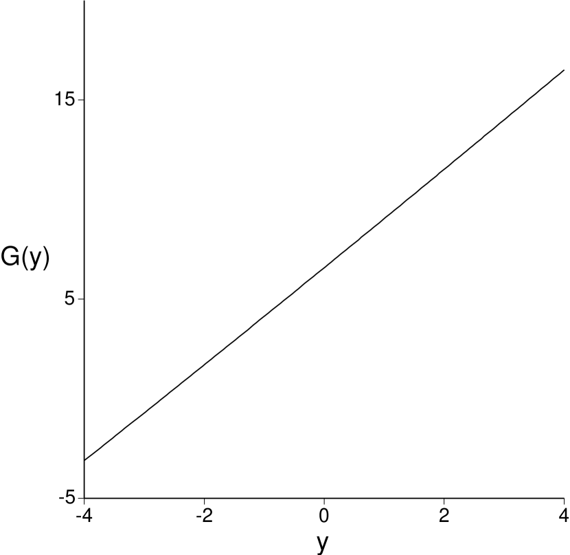
FIG. 2.: A plot of the universal scaling function $G(y)$ defined in (50). Notice that it is smooth at $y=0$. It is analytic for all real $y>-2\pi$.

FIG. 3.: As in Fig 1, but for the case where the quantum critical point is above its upper-critical dimension. Now properties are controlled by the value of the coupling $u_{0}$, associated with the least irrelevant operator involving quantum-mechanical interactions; we denote its scaling dimension as $-\theta_{u}$ ($\theta_{u}>0$). The crossover boundaries on either side of region II, and the phase transition line $T=T_{c}(t)$, now scale as $T\sim(|t|/u_{0})^{z\nu/(1+\theta_{u}\nu)}$. The boundary between regions Ia and Ib scales as $T\sim t^{z\nu}$. The expansion is now in powers of the bare coupling $u_{0}$, and as before, classical tricritical crossover functions are needed in the shaded region $|T-T_{c}(t)|\ll T_{c}(t)$. For more discussion on the regions see the discussion below Eqn (105).

FIG. 4.: A plot of the universal scaling function $\Upsilon(y)$, defined in (109), for $d=3$. Notice that it is smooth at $y=0$. It is analytic for all real $y>-2\pi$.

REFERENCES

- [1] J.A. Hertz, Phys. Rev. B 14, 525 (1976).
- [2] M. Suzuki, Prog. Theor. Phys. 56, 1454 (1976).
- [3] I.D. Lawrie, J. Phys. C 11, 1123 (1978); ibid 11, 3857 (1978).
- [4] K.K. Singh, Phys. Rev. B 12, 2819 (1975); ibid 17, 324 (1978).
- [5] R.J. Creswick and F.W. Wiegel, Phys. Rev. A 28, 1579 (1983).
- [6] M. Rasolt, M.J. Stephen, M.E. Fisher and P.B. Weichmann, Phys. Rev. Lett. 53, 798 (1984); P.B. Weichmann, M. Rasolt, M.E. Fisher, and M.J. Stephen, Phys. Rev. B 33, 4632 (1986).
- [7] D.S. Fisher and P.C. Hohenberg, Phys. Rev. B 37, 4936 (1988); see also V.N. Popov, Functional Integrals in Quantum Field Theory and Statistical Physics, D. Reidel (Boston), 1983.
- [8] S. Chakravarty, B.I. Halperin, and D.R. Nelson, Phys. Rev. B 39, 2344 (1989).
- [9] S. Sachdev and J. Ye, Phys. Rev. Lett. 69, 2411 (1992); A.V. Chubukov and S. Sachdev, Phys. Rev. Lett. 71, 169 (1993); A.V. Chubukov, S. Sachdev and J. Ye, Phys. Rev. B 49, 11919 (1994).
- [10] A.J. Millis, Phys. Rev. B 48, 7183 (1993).
- [11] A. Sokol and D. Pines, Phys. Rev. Lett. 71, 2813 (1993).
- [12] S. Sachdev, T. Senthil, and R. Shankar, Phys. Rev. B 50, 258 (1994).
- [13] M.A. Continentino, Phys. Rep. 239, 179 (1994).
- [14] S. Sachdev, Z. Phys. B 94, 469 (1994).
- [15] U. Zulicke and A.J. Millis, Phys. Rev. B 51, 8996 (1995).
- [16] S. Sachdev, A.V. Chubukov and A. Sokol, Phys. Rev. B, 51, 14874 (1995).
- [17] L.B. Ioffe and A.J. Millis, Phys. Rev. B, 51, 16151 (1995).
- [18] J. Ye, S. Sachdev, and N. Read, Phys. Rev. Lett. 70, 4011 (1993); N. Read, S. Sachdev and J. Ye, Phys. Rev. B, 52, 384 (1995).
- [19] S. Sachdev, N. Read and R. Oppermann, Phys. Rev. B, 52, 10286 (1995).
- [20] A.M. Sengupta and A. Georges, Phys. Rev. B, 52, 10295 (1995).
- [21] S. Sachdev in the Proceedings of the 19th IUPAP International Conference on Statistical Physics, Xiamen, China, July 31 - August 4 1995, World Scientific, Singapore (1996); Report No.cond-mat/9508080.
- [22] D. O’Connor and C.R. Stephens, Nucl. Phys. B360, 297 (1991); Proc. Roy. Soc. Lond. A 444, 287 (1994); Int. J. Mod. Phys. A 9, 2805 (1994); F. Freire, D. O’Connor, and C.R. Stephens, J. Stat. Phys. 74, 219 (1994) and Report No. cond-mat/9503110.
- [23] E. Brezin, J.C. Le Guillou and J. Zinn-Justin in Phase Transitions and Critical Phenomena , vol. 6, C. Domb and M.S. Green eds., Academic Press, London (1976).
- [24] Quantum Field Theory and Critical Phenomena by J. Zinn-Justin, Oxford University Press, Oxford (1993).
- [25] P.C. Hohenberg and B.I. Halperin, Rev. Mod. Phys. 49, 435 (1977).
- [26] S. Sachdev, Nucl. Phys. B 464, 576 (1996); K. Damle and S. Sachdev, Phys. Rev. Lett. 76, 4412 (1996).
- [27] M. Luscher, Phys. Lett. 118B, 391 (1982).
- [28] E. Brezin and J. Zinn-Justin, Nucl. Phys. B257, 867 (1985).
- [29] J. Rudnick, H. Guo and D. Jasnow, J. Stat. Phys. 41, 353 (1985).
- [30] Field Theory by P. Ramond, Benjamin Cummings, Reading MA (1981).
- [31] Modern Theory of Critical Phenomena by S.-K. Ma, Benjamins Cummings, Reading MA (1976).
- [32] D.R. Nelson and J. Rudnick, Phys. Rev. Lett. 35, 178 (1975); A.D. Bruce and D.J. Wallace, J. Phys. A, 9, 1117 (1976).
- [33] T. Vojta, D. Belitz, R. Narayan and T.R. Kirkpatrick, cond-mat/9510146; T.R. Kirkpatrick and D. Belitz, cond-mat/9601008.
- [34] D. O’Connor, C.R. Stephens, and A.J. Bray, cond-mat/9601146.