Spatial organization in cyclic Lotka-Volterra systems

Abstract

We study the evolution of a system of $N$ interacting species which mimics the dynamics of a cyclic food chain. On a one-dimensional lattice with $N<5$ species, spatial inhomogeneities develop spontaneously in initially homogeneous systems. The arising spatial patterns form a mosaic of single-species domains with algebraically growing size, $\ell(t)\sim t^{\alpha}$, where $\alpha=3/4$ (1/2) and 1/3 for $N=3$ with sequential (parallel) dynamics and $N=4$, respectively. The domain distribution also exhibits a self-similar spatial structure which is characterized by an additional length scale, ${\cal L}(t)\sim t^{\beta}$, with $\beta=1$ and 2/3 for $N=3$ and 4, respectively. For $N\geq 5$, the system quickly reaches a frozen state with non interacting neighboring species. We investigate the time distribution of the number of mutations of a site using scaling arguments as well as an exact solution for $N=3$. Some possible extensions of the system are analyzed.

PACS numbers: 02.50.Ga, 05.70.Ln, 05.40.+j

I Introduction

The classic Lotka-Volterra equations[1, 2, 3] mimic the dynamics of interacting species such as predator-prey systems. These equations are rather successful in predicting density oscillations which are known to exist in Nature. For spatially inhomogeneous situations, Lotka-Volterra equations[4] are straightforwardly generalized to diffusion-reaction equations[5]; these equations were widely applied to more complex ecological processes. However, such an approach ignores spatial correlations and therefore fails to predict the development of spatial heterogeneities in initially homogeneous systems. For chemical processes, the crucial role that spatial heterogeneities play in governing the kinetics has been appreciated over the past decade, see e.g.[6] and references therein. Therefore, in low spatial dimensions the mean-field like rate equations approach (analog of the Lotka-Volterra equations in chemical kinetics) fails to provide the correct asymptotic behavior. Indeed, a homogeneous initial state evolves to a strongly heterogeneous state, namely to a coarsening mosaic of reactants which confines the actual microscopic reaction to the interfacial regions between domains, and therefore the kinetics are significantly slowed down. Similar spatial organization was recently reported in Lotka-Volterra systems[7, 8, 9, 10, 11]. However, theoretical understanding of these systems is still incomplete.

In this study, we consider the evolution of an $N$ species food chain, where every species plays the role of prey and predator simultaneously. The food chain is thus assumed to be cyclic; e.g., in the 3-species system, $A$ eats $B$, $B$ eats $C$, and $C$ eats $A$. Every “eating” event leads to duplication of the winner and elimination of the loser, therefore the 3-species food chain is symbolized by the reaction scheme

$$A+B\to 2A,\quad B+C\to 2B,\quad C+A\to 2C.$$ (1)

The corresponding stochastic process is well defined on a lattice, where the interaction is restricted to nearest neighbor sites. Initially, every lattice site is assumed to be occupied; clearly, the lattice then remains fully occupied.

Given the simplicity of the reaction process (1), one anticipates that it can provide a caricature description of a number of phenomena in Nature and Society. One example is the voter model[12, 13], which is applicable to chemical reactions on catalytic surfaces[14, 15]. This model is equivalent to the 2-species model, which is described by the reaction scheme $A+B\to 2A$ or $A+B\to 2B$ (both channels are equally probable). The subsequent cyclic $N$-species generalization is also called the $N$-color cyclic voter model[16].

The rest of this paper is organized as follows. In section II, we discuss predator-prey dynamics in infinite dimensions (mean-field) and a relationship to Nambu mechanics. Section III examines interface dynamics in one dimension. We analyze the corresponding rate equations and show that spatial organization into an alternating mosaic of growing domains occurs for $N<5$ only. While the qualitative predictions made in Sec. III are correct, the quantitative predictions fail. In Sec. IV, we further analyze the interface dynamics using primarily scaling arguments and numerical simulations for the most interesting cases, $N=3$ and 4. We consider both sequential and parallel dynamics evolution rules, as the system may be sensitive to such rules. Section V studies the dynamics of mutations and quantities such as the fraction of persistent sites. In sections III-V we focus on symmetric and uncorrelated initial conditions where all the $N$ species have an initial density of $1/N$. In section VI, we describe several natural generalizations of the model to asymmetric initial concentrations, symmetric interaction rules and reaction-diffusion descriptions. Section VII discusses our results within the general framework of coarsening phenomena. A Summary is presented in section VIII.

II DYNAMICS IN INFINITE DIMENSION

Since we are interested in the role of spatial correlations, we study primarily the extreme case of one dimension, where spatial inhomogeneities are most pronounced. As a preliminary step, however, it proves useful to examine the opposite extreme where no correlations are present, i.e., the cyclic Lotka-Volterra system on a complete graph. On this structure, all sites are neighbors and the spatial structure is irrelevant, i.e., $d=\infty$.

Consider the 3-species Lotka-Volterra model (1). The simplest mean-field description of this model, which is exact only on a complete graph, consists of the following rate equations for the species concentrations $a(t)$, $b(t)$, and $c(t)$,

$$\dot{a} = a(b-c),$$ (2)

$$\dot{b} = b(c-a),$$ (3)

$$\dot{c} = c(a-b),$$ (4)

where the over-dot denotes the time derivative. These equations obey the trivial conservation law, $a+b+c=1$, that merely reflects particle conservation. There is an additional hidden integral, $abc={\rm const}$. The existence of these two integrals allows us to describe the behavior of the system without actually solving Eqs. (2). Clearly, a generic solution to Eqs. (2) is periodic; this solution can be expressed through elliptic functions. There are also simpler exceptional solutions, corresponding to situations when one of the concentrations is zero. In this case, the solution approaches an attracting point; e.g., if $c=0$, one readily finds that $a(t)\to 1$ and $b(t)\to 0$ when $t\to\infty$, while the approach towards these limiting values is exponential in time.

Several authors notified that some Lotka-Volterra equations admit a Hamiltonian structure[17]. However, even in very simple situations the Hamiltonian structure can be impossible, e.g., it is clearly the case when the number of species is odd as in the 3-species cyclic Lotka-Volterra system. We now describe a more intricate relationship between the 3-species Lotka-Volterra equations and Nambu mechanics. Nambu mechanics[18, 19] is a generalized Hamiltonian mechanics where the usual pair of canonical variables of the Hamiltonian are replaced by a triplet of coordinates. Nambu formulated these dynamics via the ternary operation, the Nambu bracket, replacing the binary Poisson bracket. The Nambu bracket, $\{f,g,h\}$, satisfies the usual skew-symmetry, the Leibniz rule, and the generalized Jacobi identity[19]. Let $c_{1},c_{2},c_{3}$ denote the coordinates. The canonical Nambu bracket is

$$\{f_{1},f_{2},f_{3}\}={\partial(f_{1},f_{2},f_{3})\over\partial(c_{1},c_{2},c_{3})},$$ (5)

where the right-hand side is the Jacobian. Similarly, one can define the canonical $N$-ary Nambu bracket, ${\partial(f_{1},\ldots,f_{N})\over\partial(c_{1},\ldots,c_{N})}$, which is identical to the canonical Poisson bracket for $N=2$. To define the Hamiltonian dynamics one needs a special function $H$; then, an arbitrary function $f$ evolves according to Hamilton’s equations of motion, $\dot{f}=\{f,H\}$. To define the Nambu dynamics, one needs two “Hamiltonians” denoted by $H_{1}$ and $H_{2}$. Nambu’s equations of motion read

$$\dot{f}=\{f,H_{1},H_{2}\}.$$ (6)

A few systems possessing hidden integrals of motion were immersed in the framework of Nambu mechanics[18, 19, 20, 21]. Surprisingly, Eqs. (2) provide a very simple additional example. Indeed, writing $a=c_{1},b=c_{2},c=c_{3}$, using the integrals of Eqs. (2) as the Hamiltonians, $H_{1}=a+b+c$ and $H_{2}=abc$, choosing the canonical Nambu bracket (5), and specializing Nambu equations (6) to $f=a,b,c$, we recover Eqs. (2).

One can investigate Lotka-Volterra models for a greater number of species. We checked that for $N=4$, one can still recast the corresponding Lotka-Volterra equations for the concentrations $c_{j},1\leq j\leq 4$, into the framework of Nambu mechanics with canonical Nambu bracket and the Hamiltonians $H_{1}=c_{1}+c_{2}+c_{3}+c_{4}$, $H_{2}=c_{1}c_{3}$, and $H_{3}=c_{2}c_{4}$. It would be interesting to establish a Nambu-type formulation (if any) for the cyclic $N$-species model with arbitrary $N$. On the complete graph, the corresponding rate equations are

$$\dot{c}_{k}=c_{k}\left(c_{k+1}-c_{k-1}\right)\equiv F_{k},$$ (7)

for $k=1,\ldots,N$, and the addition and subtraction of the index are taken modulo $N$. Eqs. (7) appear not only in mathematical biology[2] but also in plasma physics where they describe the fine structure of the spectrum of Langmuir oscillations[22] (the system (7) with $-\infty<k<\infty$ is also called “Langmuir lattice”).

The possible existence of the Nambu formulation implies that Eqs. (7) should satisfy the Liouville condition[23], $\sum_{k}\partial F_{k}/\partial c_{k}=0$. An elementary computation shows that this necessary condition is indeed satisfied. Another necessary condition is the existence of $N-1$ independent integrals of motion. For the general $N$-species cyclic Lotka-Volterra model one easily finds two such integrals,

$$H_{1}=\sum_{j=1}^{N}c_{j},\quad{\rm and}\quad H_{2}=\prod_{j=1}^{N}c_{j}.$$ (8)

When the number of species is even, $N=2P$, the products of even and odd concentrations separately,

$$H_{3}=\prod_{j=1}^{P}c_{2j},\quad H_{4}=\prod_{j=1}^{P}c_{2j-1},$$ (9)

are also conserved so there are at least three independent integrals of motion: $H_{1}$, $H_{3}$, and $H_{4}$. Generally, $[N/2]$ integrals of Eqs. (7) involving polynomials of $c_{j}$ and $\ln c_{j}$ are known (see e.g.[24, 25] and references therein). However, for the $N$-species cyclic Lotka-Volterra model to admit the Nambu formulation, $N-1$ independent integrals are necessary, and it is not clear whether a Nambu structure exists for $N\geq 5$.

Although we have not yet derived new results with the help of the Nambu structure, its richness may be useful in understanding the evolution of cyclic Lotka-Volterra systems.

III RATE EQUATIONS FOR 1D INTERFACE DYNAMICS

The infinite dimensional analysis fails to describe the dynamics of the actual stochastic process in low dimensions. For example, while the sum $H_{1}=\sum_{j}c_{j}$ is conserved, the product $H_{2}=\Pi_{j}c_{j}$ is not a conserved quantity in 1D. Furthermore, the structure of Eqs. (2) does not address fluctuations in the spatial distribution of interacting populations. For $N<5$, we shall see that the spatial structure evolves forever, single-species domains arise and grow indefinitely, and the process exhibits coarsening. In other words, equilibrium is never achieved and instead a networks of domains develops. The domain patterns are self-similar, i.e., the structure at later times and at earlier times differ only by a global change of scale. Such a behavior is a signature of dynamical scaling.

In the following section, we study the motion of “domain walls”, namely, interfaces separating domains of different species. For the $N$ species process a bond connecting two sites is an interface bond if the corresponding two sites are occupied by two different species. Thus, there are $N-1$ independent types of interfaces, of which $N-3$ are immobile and 2 are mobile. For symmetric initial conditions ($c_{i}(0)=1/N$), the different types of interface bonds are present with initial concentration equal to $1/N$ (with probability $1/N$ a given bond does not contain an interface). Interfaces move and react according to $N$-dependent rules defined below. For large $N$, most interfaces are immobile and the system quickly reaches a state where all mobile interfaces are eliminated.

A 2-Species

Consider the simplest case of $N=2$, where there are two equivalent interfaces ($AB$ and $BA$), denoted by $I$. An isolated interface performs a random walk, i.e., it hops to one of its nearest neighbors. When two interfaces meet they annihilate. The corresponding reaction scheme is therefore $I+I\to\emptyset$. Assuming that neighboring interfaces are uncorrelated, we arrive at the binary reaction equation

$$\dot{I}=-4I^{2}.$$ (10)

The hoping rate was taken as unity without loss of generality. Solving this equation subject to the initial conditions $I(0)=1/2$ gives

$$I(t)={1\over 2+4t}.$$ (11)

The system evolves into a mosaic of alternating domains $AABBBAAABBB$. The typical size of a domain grows linearly with time, ${\cal L}(t)\sim t$.

B 3-species

In the case $N=3$, there are two types of interfaces, right moving ($AB$, $BC$, and $CA$), and left moving ($BA$, $CB$, and $AC$), denoted by $R$ and $L$, respectively. Starting with a symmetric initial distribution, all right (left) interfaces are equivalent. When a right moving interface meets a left moving one, they annihilate $R+L\to\emptyset$. When a right moving interface overtakes another right moving interface, they give rise to a left moving interface, $R+R\to L$, and similarly, $L+L\to R$. The corresponding rate equations are

$$\dot{R} = -2R^{2}-2RL+L^{2},$$ (12)

$$\dot{L} = -2L^{2}-2RL+R^{2}.$$ (13)

The interface concentration is readily found,

$$R(t)=L(t)={1\over 3+3t}.$$ (14)

The behavior is similar to the case $N=2$, as the resulting spatial pattern form a mosaic of single-species domains whose average size is ${\cal L}\sim t$. The previous analysis implicitly assumes that interfaces hop one at a time, namely sequential dynamics. Alternatively, one can consider simultaneous hoping, or parallel dynamics. Here interfaces move ballistically, and thus, interfaces moving with the same velocity do not interact. The reaction scheme is $R+L\to\emptyset$, and the rate equations read $\dot{R}=\dot{L}=-2RL$. The resulting interface concentrations $R(t)=L(t)=1/(3+2t)$ differ only slightly from Eq. (14).

C 4-species

In the 4-species model there appear static interfaces denoted by $S$ ($AC$, $BD$, $CA$, and $DB$), in addition to the previously defined right moving interfaces ($AB$, $BC$, $CD$, and $DA$), and left moving interfaces ($BA$, $CB$, $DC$, and $AD$). Interfaces react upon collision according to the rules $R+L\to\emptyset$, $R+S\to L$, $R+R\to S$, $L+L\to S$, and $S+L\to R$, resulting in the following rate equations

$$\dot{R}= - 2R^{2}-2RL-RS+SL,$$ (15)

$$\dot{L}= - 2L^{2}-2RL-SL+RS,$$ (16)

$$\dot{S}= R {}^{2}+L^{2}-RS-SL.$$ (17)

Solving these equations subject to the appropriate initial conditions gives

$$R(t)=L(t)={1\over 4+4t},\quad S(t)={1\over\sqrt{4+4t}}-{1\over 4+4t}.$$ (18)

Different rules govern the decay of static and mobile interfaces, and consequently, the coarsening process is characterized by two intrinsic length scales. The typical distance between two static interfaces, $t^{1/2}$, grows slower than the distance between two moving interfaces, $t$. A nontrivial spatial organization occurs in which large “superdomains” contain many domains of alternating noninteracting ($AC$ or $BD$) species, $BAAACCAAACCCAAAD$. We denote the typical domain size by $\ell\sim t^{1/2}$ and the typical superdomain size by ${\cal L}\sim t$. The typical number of noninteracting domains inside a superdomain grows as ${\cal L}/\ell\sim t^{1/2}$. Such an organization is a consequence of the existence of noninteracting species, which first occurs at $N=4$.

It is useful to consider parallel dynamics as well. Again, the reaction scheme is altered only in that the interfaces moving in the same direction do not interact. The reaction scheme, $R+L\to\emptyset$, $R+S\to L$, and $S+L\to R$, is described by the following rate equations

$$\dot{R}= - 2RL-RS+SL,$$ (19)

$$\dot{L}= - 2RL-SL+RS,$$ (20)

$$\dot{S}= - RS-SL.$$ (21)

Solving the rate equations we arrive at

$$R(t)=L(t)=S(t)={1\over 4+2t}.$$ (22)

Interestingly, when $N=4$ coarsening is sensitive to the details of the dynamics. Parallel dynamics is governed by a single length scale, in contrast with the two scales underlying sequential dynamics.

D 5-species

In the 5-species case there are two types of stationary interfaces, $S_{R}$ ($AC,BD,CE,DA,EB$) and $S_{L}$ ($AD,BE,CA,DB,EC$), in addition to the right and left moving interfaces, $R$ ($AB,BC,CD,DE,EA$) and $L$ ($BA,CB,DC,AD,AE$). The reaction process is symbolized by $R+L\to\emptyset$, $R+S_{L}\to L$, $R+S_{R}\to S_{L}$, $S_{R}+L\to R$, $S_{L}+L\to S_{R}$, $R+R\to S_{R}$, and $L+L\to S_{L}$. In other words, when a moving interface hits a stationary interface of the same kind, the outcome is a stationary interface of the opposite kind; when a moving interface hits a stationary interface of the opposite kind, a dissimilar moving interface emerges. Collisions between similar moving interfaces produce stationary interfaces of the same kind, and thus, the obvious notations $S_{L}$ and $S_{R}$. For the 5-species model with sequential dynamics, the rate equations read

$$\dot{L}= - 2RL-LS_{L}-LS_{R}+RS_{L}-2L^{2},$$ (23)

$$\dot{R}= - 2RL-RS_{L}-RS_{R}+LS_{R}-2R^{2},$$ (24)

$$\dot{S}_{L}= - RS_{L}-LS_{L}+RS_{R}+L^{2},$$ (25)

$$\dot{S}_{R}= - RS_{R}-LS_{R}+LS_{L}+R^{2}.$$ (26)

The reaction scheme and consequently the rate equations are invariant under the duality transformation $(R,S_{R})\longleftrightarrow(L,S_{L})$. Particularly, for $R(0)=L(0)$ and $S_{R}(0)=S_{L}(0)$, the corresponding densities remain equal forever. This condition is certainly satisfied for the symmetric initial conditions $R(0)=L(0)=S_{L}(0)=S_{R}(0)=1/5$. Therefore, $R(t)=L(t)$ and $S_{L}(t)=S_{R}(t)$, and in what follows we shall use the notations $M(=R=L)$ for mobile interfaces and $S(=S_{L}=S_{R})$ for stationary interfaces. Thus, the four rate equations reduce to a pair of rate equations:

$$\dot{M}=-4M^{2}-SM,\quad\dot{S}=M^{2}-SM.$$ (27)

These equations can be linearized by introducing a modified time variable, $T(t)=\int_{0}^{t}M(t^{\prime})dt^{\prime}$. Using the notation ${}^{\prime}\equiv d/dT$, we rewrite the governing equations as

$$M^{\prime}=-4M-S,\quad S^{\prime}=M-S.$$ (28)

Solving these equations gives

$$M(T) ={1\over 5}\left(\lambda_{+}e^{-\sqrt{5}\lambda_{+}T}-\lambda_{-}e^{-\sqrt{5}\lambda_{-}T}\right),$$ (29)

$$S(T) ={1\over 5}\left(\lambda_{+}e^{-\sqrt{5}\lambda_{-}T}-\lambda_{-}e^{-\sqrt{5}\lambda_{+}T}\right),$$ (30)

with the shorthand notations, $\lambda_{\pm}=(\sqrt{5}\pm 1)/2$. Here, the moving interfaces are depleted at $T_{\infty}=2(\ln\lambda_{+})/\sqrt{5}$. The density of static interfaces approaches a finite value, $S(\infty)={1\over 5}\left(\lambda_{+}^{2-\sqrt{5}}-\lambda_{-}^{2+\sqrt{5}}\right)\cong 0.152477$, so the average domain size in the frustrated state is ${\cal L}(\infty)=1/2S(\infty)\cong 3.27918$. In terms of the actual time $t$, the density of moving interfaces decays exponentially, $R(t)\propto e^{-S(\infty)t}$. Contrary to the previous cases, $N<5$, no coarsening occurs and the system quickly approaches a frozen state of short noninteracting same-species domains separated by stationary interfaces.

A similar picture is found for parallel dynamics as well. Here, the reaction process is $R+L\to\emptyset$, $R+S_{L}\to L$, $R+S_{R}\to S_{L}$, $S_{R}+L\to R$, $S_{L}+L\to S_{R}$, and the rate equations are

$$\dot{L}= - 2RL-LS_{L}-LS_{R}+RS_{L},$$ (31)

$$\dot{R}= - 2RL-RS_{L}-RS_{R}+LS_{R},$$ (32)

$$\dot{S}_{L}= - RS_{L}-LS_{L}+RS_{R},$$ (33)

$$\dot{S}_{R}= - RS_{R}-LS_{R}+LS_{L}.$$ (34)

The useful duality relation, $(R,S_{R})\longleftrightarrow(L,S_{L})$, still applies, so there are only two independent interface concentrations, $M$ and $S$, which evolve according to the following rate equations

$$\dot{M}=-2M^{2}-MS,\quad\dot{S}=-MS.$$ (35)

The calculation is very similar to the sequential case, and we merely quote the results

$$M(T)={2e^{-2T}-e^{-T}\over 5},\quad S(T)={e^{-T}\over 5}.$$ (36)

The limit $t\to\infty$ corresponds to $T\to T_{\infty}=\ln 2$. We find that the density of static interfaces saturates at a finite value, $S(\infty)=1/10$, while the density of moving interfaces decays exponentially in time, $M(t)\propto e^{-S(\infty)t}=e^{-t/10}$. The average size of a domain in the frozen state is ${\cal L}(\infty)=1/2S(\infty)=5$.

To summarize, both for parallel and sequential dynamics the rate equations predict coarsening when the number of species is sufficiently small, $N<5$, and fixation for a large number of species, $N\geq 5$. When fixation occurs, each site attains a final state while for $N\leq 4$ the state of any site continues to change, although the frequency of changes decreases with time. It is remarkable that the rate equation approach which neglects spatial correlations between interfaces correctly predicts the marginal food chain length for fixation, $N_{c}=5$, as has been proved rigorously for both sequential dynamics [16] and parallel dynamics [26].

In the coarsening cases, $N<5$, both for the two- and three-species case the average domain size $\ell(t)$ grows linearly with time independent of the dynamics. In the 4-species case, however, the rate equation theory predicts linear growth $\ell(t)\sim t$ for parallel dynamics, and slower ”diffusive” growth $\ell(t)\sim\sqrt{t}$ for sequential dynamics. In the latter case, the larger linear scale still exists and it characterizes the typical distance between two mobile interfaces.

IV COARSENING DYNAMICS IN ONE DIMENSION

The above rate equation theory successfully predicts the fixation transition at $N_{c}=5$ in agreement with rigorously known results [16, 26]. If one assumes that the average concentration of each species is conserved throughout the process, which is clearly correct at least in the case of equal initial concentrations, one can find a simple argument for a lower bound on the marginal food chain length $N_{c}$. A frozen chain consists of alternating domains of noninteracting species. For $N=2,3$ such a chain is impossible since all species interact. For $N=4$, frozen chains are filled by either $A$ and $C$ species or $B$ and $D$ species thereby violating the conservation of the densities. [Note, however, that for $N=4$ in finite systems, density fluctuations could drive the system towards a final frozen configuration]. For $N\geq 5$, a frozen chain conserving the densities is possible and thus $N_{c}\geq 5$. Given the kinetics predicted by the mean-field rate equation approach usually proceeds with a faster rate than actual kinetics[6], one can anticipate that the threshold number of different species predicted by the mean-field theory provides an upper bound for the actual $N_{c}$, $N_{c}\leq 5$. This is combined with the lower bound, $N_{c}\geq 5$, to yield $N_{c}=5$.

For $N<5$, coarsening occurs and it is quite possible that the system develops significant spatial correlations. In such a case, the quantitative predictions of the rate equation theory are inaccurate.

The cyclic $N$-species Lotka-Volterra model is implemented in the following way. We consider a one-dimensional lattice of size ${\cal N}$ with periodic boundary conditions. Each site $i$ of the lattice is in a given state $N_{i}$ with $N_{i}=A,B,C,\dots$ In sequential dynamics, we choose randomly a site and then one of its two nearest neighbors. If the neighbor is a predator of the chosen site, the state of the latter changes to the state of the predator. Otherwise, the state of the site remains the same. Time is incremented by $1/{\cal N}$ after each step. For parallel dynamics, all sites are updated simultaneously and change their state if one of their nearest neighbors is their predator. This cellular automata rule has been used in [26] and it should be noted that the dynamics is fully deterministic. Coarsening behavior of the system depends on spatial fluctuations present in the initial state. For both types of dynamics, efficient algorithms keeping trace only of moving interfaces have been implemented.

Below, we present numerical findings accompanied by heuristic arguments for the coarsening dynamics in one dimension. Again, we restrict ourselves to the symmetric initial concentration. In this case the average concentration of each species remains $1/N$, despite the nonconserving microscopic evolution rules.

A 2-species

As mentioned previously, for $N=2$, interfaces perform a random walk and annihilate upon collision. This exactly soluble voter model[12] is equivalent to the one-dimensional Glauber-Ising model at zero temperature [27, 28]. The interface concentration is given by[27]

$$I(t)=e^{-4t}[I_{0}(4t)+I_{1}(4t)]/2,$$ (37)

with $I_{n}(x)$ the $n^{\rm th}$ order modified Bessel function. In the limit $t\to 0$ correlations are absent and the interface density $I(t)\cong 1/2-t$ agrees with the short time limit of Eq. (11). Asymptotically, the coarsening is much slower in comparison with the rate equation predictions, $I(t)\simeq(8\pi t)^{-1/2}$. The system separates into single species domains as follows

$$AAABBBB\underbrace{AAAA}_{\ell}BBAAA.$$ (38)

The average domain size $\ell$ exhibits a diffusive growth law $\ell(t)\sim t^{\alpha}$ with $\alpha=1/2$.

In the 2-species case, parallel dynamics is generally meaningless since it quickly leads to a chain consisting of alternate clusters with no more than two consecutive similar-species sites. All sites of the chain then change their states at each time step. However, a parallel realization of the sequential dynamics is possible if all initial distances between interfaces are even integers. In this case, the number of interfaces gradually decreases, and a behavior very similar to the sequential case emerges[29].

B 3-species

It is convenient to consider first the simpler parallel dynamics where interfaces move ballistically with velocity $\pm 1$, and annihilate upon collisions. In this well understood ballistic annihilation process[26, 30, 31, 32, 33, 34], a simple combinatorial calculation (see subsection V.C) yields the following interface density

$$R(t) = {1\over 3^{2t+1}}\left[\sum_{i=0}^{t}\left(\begin{array}[]{c}2t\\ 2i\end{array}\right)\left(\begin{array}[]{c}2t-2i\\ t-i\end{array}\right)\right.$$ (48)

$$\left.\qquad+\sum_{i=0}^{t-1}\left(\begin{array}[]{c}2t\\ 2i+1\end{array}\right)\left(\begin{array}[]{c}2t-2i-1\\ t-i\end{array}\right)\right].$$

In the long time limit, the interfaces concentration decay $R\simeq(6\pi t)^{-1/2}$ is much slower than the $t^{-1}$ decay suggested by the rate equation (14). The decay law governing the interface density can be simply understood. Consider a finite interval of size $L$ containing interfaces with initial concentration $c_{0}$. The total number of interfaces is $N=c_{0}L$. If the initial conditions are random, the difference between the number of left and right moving interfaces is roughly $\Delta N=|N_{R}-N_{L}|\sim\sqrt{N}$. At long times, all minority interfaces are eliminated and thus, the interface concentration approaches $\Delta N/L\sim(c_{0}/L)^{1/2}$. By identifying the box size with the appropriate ballistic length $L\sim Vt$, the time dependent interface concentration for an infinite system is found, $R(t)\sim(c_{0}/Vt)^{1/2}$.

The system organizes into large ballistically growing superdomains. Each superdomain contains interfaces moving in the same direction, neighboring superdomains contain interfaces moving in the opposite direction, etc. In addition to the average size of superdomains, there is an additional length scale in the problem corresponding to the distance between two adjacent similar velocity interfaces. We define these relevant length scales using the following illustrative configuration

$$B\overbrace{AABBB\underbrace{CCCC}_{\ell}AAABBCCC}^{\cal L}B,$$ (49)

The corresponding coarsening exponents, $\alpha$ and $\beta$, are defined via $\ell\sim t^{\alpha}$ and ${\cal L}\sim t^{\beta}$, respectively. For the $N=3$ with parallel dynamics we thus find $\alpha=1/2$ and $\beta=1$. Starting from an initially homogeneous state, the system develops a unique spatially organized state which is a mosaic of mosaics. Indefinitely growing superdomains contain a growing number ${\cal D}={\cal L}/\ell\sim t^{1/2}$ of cyclically arranged domains ($ABCABC$ and $CBACBA$).

We now turn to the complementary case of sequential dynamics. Interfaces perform a biased random walk and thus, the ballistic motion is now supplemented by superimposed diffusion. In addition, two parallel moving interfaces can annihilate and give birth to an opposite moving interface. It proves useful to consider the continuum version of the model where interfaces move with velocity $+V$ and $-V$ with equal probabilities, and have a diffusivity $D$. To establish the long-time behavior we assume that the system organizes into domains of right and left moving interfaces. Inside a domain, interfaces moving in the same direction can now annihilate via a diffusive mechanism, unlike the parallel case. On slower than ballistic scales, the problem reduces to diffusive annihilation, $X+X\to\emptyset$, where $X$ is either $R$ or $L$, with a density decaying as $c_{\rm diff}(t)\sim(Dt)^{-1/2}$. On ballistic scales the problem (almost) reduces to the ballistic annihilation process $R+L\to\emptyset$, with the density decay $c_{\rm ball}(t)\sim(c_{0}/Vt)^{1/2}$ as described previously. However, to describe the complete ballistic-diffusion annihilation, one cannot use the initial concentration $c_{0}$ since it is constantly reduced by diffusive annihilation. Therefore, we replace the initial concentration $c_{0}$ with the time dependent concentration $c_{\rm diff}(t)$, and we find [35, 36] $c\sim(DV^{2}t^{3})^{-1/4}$ which in particular implies

$$\ell\sim t^{3/4}.$$ (50)

This result is quite striking since separately both annihilation processes, diffusion-controlled and ballistic-controlled, give the same coarsening exponent 1/2, so one expects that their combination does not change the behavior while in fact it enhances the coarsening exponent to 3/4. The resulting spatial structure is similar to the parallel case, Eq. (49). However, the smaller length scale is now a geometric average of a diffusive and a ballistic scale as follows from Eq. (50), while the larger scale remains unchanged, ${\cal L}\sim t$.

We have performed Monte Carlo simulations for 100 realizations on a lattice of size $10^{6}$, for times up to $t\simeq 10^{6}$. Results are shown in the Fig. 1. The interface concentration decays algebraically, $R\propto t^{-\alpha}$ with an exponent $\alpha\cong 0.79$. A careful analysis shows that the local slope $\alpha(t)=d\ln c(t)/d\ln t$ should asymptotically approach the value $-3/4$. It is possible that this finite time effect can be attributed to the recombination reaction ($R+R\to L$), which is not an annihilation reaction. Nevertheless, a single $L$-interface inside an $R$-domain is quickly annihilated by nearest $R$-interface, and therefore recombination is asymptotically equivalent to annihilation. We expect that as $t\to\infty$, the coarsening exponent is indeed $\alpha=3/4$.

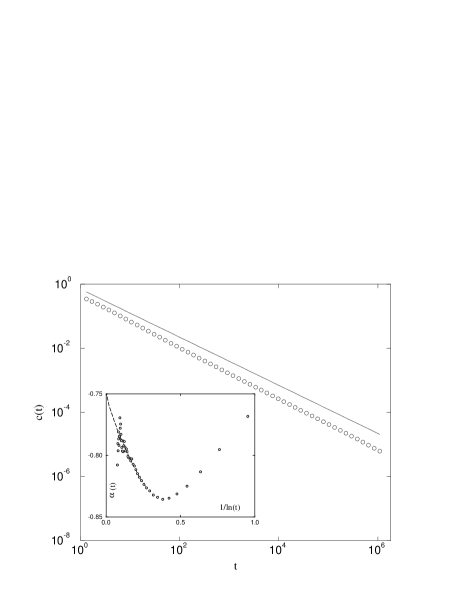
FIG. 1.: The concentrations of interfaces as a function of time for the 3-species model and a sequential dynamics in a log-log plot. A line of slope $3/4$ is shown as a reference. The insert shows the local exponent $\alpha(t)$ as a function of $1/\ln t$. A limiting value of $\alpha\rightarrow 3/4$ is plausible.

To summarize, the resulting spatial patterns in the $N=3$ case consist of superdomains of cyclically arranged domains as in Eq. (49). The larger length scale is ballistic, ${\cal L}\sim t$, while the smaller length scale is sensitive to the microscopic details of the dynamics: $\ell\sim t^{1/2}$ for parallel dynamics and $\ell\sim t^{3/4}$ for sequential dynamics.

C 4-species

For the 4-species cyclic Lotka-Volterra model, numerical simulations indicate that parallel and sequential dynamics are asymptotically equivalent and that the domain structure is qualitatively similar to the predictions of the sequential rate equations, $M(t)\ll S(t)$. We use heuristic arguments to obtain the values of the coarsening exponents $\alpha$ and $\beta$, characterizing the density decay of mobile $M(t)\sim t^{-\alpha}$, and static $S(t)\sim t^{-\beta}$ interfaces.

Given the equivalence of parallel and sequential dynamics, we restrict ourselves to the simpler former dynamics. What is the spatial structure in the long time limit? Since $M(t)\ll S(t)$ (here and below $M(t)=R(t)=L(t)$ denotes the density of moving interfaces), we assume an alternating spatial structure of “empty” regions (with no more than one moving interface) and “stationary” regions (with many stationary interfaces inside any such region). If the interface densities obey scaling, then the size of the empty and the stationary regions should be comparable. The typical size of an empty or a stationary region is therefore of the order of $M^{-1}$. The typical number of stationary interfaces inside a stationary region is of the order of $S/M$. The evolution proceeds as follows: A moving interface hits the least stationary particle and bounces back (since $R+S\to L$ and $S+L\to R$). Then this interface hits the least stationary particle of the neighboring stationary region, and bounces back again. This “zig-zag” process continues and at some time one of these stationary regions “melts”, thereby giving birth to a larger empty region. If there is a moving particle inside merging empty region, the two moving particles quickly annihilate. If there is no such particle, the moving particle continues to eliminate stationary interfaces. This process is illustrated in Fig. 2.

FIG. 2.: Space time diagram of the interface motion in the 4-species case with parallel dynamics.

The typical time $\tau$ for a stationary region to melt is $\tau=M^{-1}\times S/M=S/M^{2}$. This melting time $\tau$ is also the typical time for annihilation of a moving interface and thus,

$$\dot{M}\sim-{M\over\tau}\sim-{M^{3}\over S}.$$ (51)

Substituting $S(t)\propto t^{-\alpha}$ and $M(t)\propto t^{-\beta}$ into Eq. (51) we get the exponent relation

$$2\beta-\alpha=1.$$ (52)

In the next section, we introduce the mutation distribution, and find an equivalence between the fraction of persistent sites and the static interface density. Using this relation and a simple solvable example, we find the exponent relation

$$\alpha+\beta=1.$$ (53)

The two exponent relations therefore imply the values $\alpha=1/3$ and $\beta=2/3$. We have simulated 100 systems of size $10^{6}$ up to times $t\simeq 10^{6}$. The results are shown in Figs. 3 and 4. We have found $S(t)\propto t^{-0.34}$, $R(t)=L(t)\propto t^{-0.69}$ for parallel dynamics, and $S(t)\propto t^{-0.35}$, $R(t)=L(t)\propto t^{-0.70}$ for sequential dynamics. We conclude that the simulation results support the above predictions.

As in the three-species case there are two relevant growing length scales. The system organizes into domains of alternating noninteracting species with a typical size $\ell\sim t^{1/3}$. On the other hand, active interfaces are separated by a typical distance of ${\cal L}\sim t^{2/3}$, according to the following illustration

$$B\overbrace{AACCCAAA\underbrace{CCCC}_{\ell}AACCAAACCC}^{{\cal L}}D.$$ (54)

In any finite lattice, density fluctuations drive the system towards a final frozen or “poisoned” configuration, i.e. configuration filled by either $A$ and $C$, or $B$ and $D$. This poisoning happens when the size of superdomains becomes of the order of lattice size. The poisoning time is therefore proportional to ${\cal N}^{3/2}$ for an ${\cal N}$-site chain.

FIG. 3.: The concentrations of the moving interfaces as a function of time for the 4-species cyclic Lotka-Volterra model with sequential dynamics (diamonds) and with parallel dynamics (circles). The slope give the exponents $\beta_{\rm seq}=0.70$ and $\beta_{\rm par}=0.69$. A line of slope $2/3$ is shown as a reference.

FIG. 4.: The concentrations of the stationary interfaces as a function of time for the 4-species model for sequential dynamics (diamonds) and parallel dynamics (circles). The slope give the exponents $\alpha_{\rm seq}=0.35$ and $\alpha_{\rm par}=0.34$. A line of slope $1/3$ is shown as a reference.

We stress that a 3-velocity ballistic annihilation model, $R+L\to\emptyset,R+S\to\emptyset,S+L\to\emptyset$, has been recently investigated [32, 33, 34, 35], and the symmetric case, $R\equiv L$, has been solved exactly [34]. For the special initial condition, $R(0)=L(0)=3S(0)/2$, a surprisingly similar behavior $R(t)\sim S(t)\sim t^{-2/3}$ occurs. It would be interesting to establish a relationship between this solvable ballistic annihilation model and the interface motion in the 4-species process.

D 5-species

For the 5-species cyclic Lotka-Volterra model, it is well known that the system approaches a frozen state[16, 26]. The kinetics approach towards saturation has not been established, though.

We now present a heuristic argument for estimating the concentration decay of the mobile interfaces. Since the density of mobile interfaces rapidly decreases while the density of stationary interfaces remains finite we can ignore collisions between mobile interfaces. Thus we should estimate the survival probability of a mobile interface in a sea of stationary ones. There are two reactions in which moving interfaces survive although they change their type, $R+S_{L}\to L$ and $L+S_{R}\to R$. Thus, a right moving interface is long lived in the following environment

$$\cdots S_{R}S_{R}S_{R}S_{R}MS_{L}S_{L}S_{L}S_{L}\cdots$$ (55)

Clearly, in such configurations the zig-zag reaction process takes place. The moving interface travels to the right during a time $t_{0}\sim 1/c_{0}v_{0}$, eliminates a stationary interface and travels to the left a time of order $2t_{0}$, eliminates an interface and travels back to the right, etc. Thus, to eliminate $N_{s}$ interfaces, the moving interface should spend a time of order $t\simeq t_{0}\sum_{i=1}^{N_{s}}i=t_{0}N_{s}(N_{s}+1)/2$. Therefore, the number of stationary interfaces $N_{s}(t)$ eliminated by a moving interface scales with time as $N_{s}(t)\sim\sqrt{c_{0}v_{0}t}$. Configurations of the type (55) are encountered with probability $\propto e^{-N_{s}}$ with $N_{s}$ the configuration length, and thus, the density of moving interfaces exhibits a stretched exponential decay,

$$M(t)\propto e^{-{\rm const.}\times\sqrt{c_{0}v_{0}t}}.$$ (56)

The stretched exponential behavior (56) is expected to appear for arbitrary $N\geq 5$. When the number of interfaces exceeds the threshold value, $N>5$, stationary interfaces of “intermediate” types arise, the crossover from initial exponential behavior to the asymptotic stretched exponential behavior is shifted to larger times and therefore harder to observe numerically. For the threshold number of species, however, we have found a convincing agreement between the theoretical prediction of Eq. (56) and numerical results (see Fig. 5). Finally we note that the actual kinetics (56) is slower than the mean-field counterpart, $M_{\rm MFT}(t)\propto e^{-t}$, due to spatial correlations.

FIG. 5.: The concentration of moving interfaces as a function of the square root of time in linear-log plot for the 5-species cyclic Lotka-Volterra model with sequential dynamics.

V DYNAMICS OF MUTATIONS

Consider a lattice site occupied by some species, say $A$. What is the probability that this site has been occupied by the same species during the time interval $(0,t)$? Otherwise, what is the fraction of $A$ sites which never “mutated”? We denote the fraction of “persistent” $A$ species by $A_{0}(t)$; $B_{0}(t)$, $C_{0}(t)$, etc. are defined analogously. We can further generalize these probabilities to define, e.g., $A_{n}(t)$, the fraction of sites that have undergone exactly $n$ mutations during the time interval $(0,t)$. We start by analyzing these quantities on the mean-field level and then describe exact, scaling, and numerical results in one dimension.

A Mean-Field Theory

Let us investigate the 3-species cyclic Lotka-Volterra on the complete graph; the generalization to the $N$-species case is straightforward. The rate equations describing the evolution of the mutation distribution $A_{n}(t)$ are

$$\dot{A}_{3n}= aA_{3n-1}-cA_{3n},$$ (57)

$$\dot{A}_{3n+1}= cA_{3n}-bA_{3n+1},$$ (58)

$$\dot{A}_{3n+2}= bA_{3n+1}-aA_{3n+2}$$ (59)

with $A_{-1}(t)\equiv 0$. Analogous equations can be written for $B_{n}(t)$ and $C_{n}(t)$ by cyclic permutations. These rate equations form an infinite set of linear equations with $a(t),b(t)$, and $c(t)$ as (time-dependent) coefficients. Therefore, the general case is hardly tractable analytically since the coefficients, i.e. solutions of Eqs. (2), are elliptic functions. We therefore restrict our attention to the symmetric case $a=b=c=1/3$, and examine $P_{n}(t)$, the total fraction of sites mutated exactly $n$ times. The quantity $P_{n}(t)$ evolves according to

$$\dot{P}_{n}=P_{n-1}-P_{n},$$ (60)

with $P_{-1}\equiv 0$ to ensure $\dot{P}_{0}=-P_{0}$. In Eq. (60) we absorbed the concentration factor 1/3 into the time-scale for convenience. Solving (60) subject to the initial condition $P_{n}(0)=\delta_{n0}$, one finds a Poissonian mutation distribution

$$P_{n}(t)={t^{n}\over n!}\,e^{-t}.$$ (61)

This mutation distribution is identical to the one found for the voter model[13] on the mean-field level.

The distribution is peaked around the average $\langle n\rangle=t$, and the width of the distribution, $\sigma$, is given by $\sigma^{2}=\langle n^{2}\rangle-\langle n\rangle=t$. In the limits, $t\to\infty$, $n\to\infty$, and $(n-t)/\sqrt{t}$ finite, $P_{n}(t)$ approaches a scaling form

$$P_{n}(t)={1\over\sigma}\Phi_{\infty}\left({n-\langle n\rangle\over\sigma}\right),$$ (62)

where the scaling distribution function $\Phi_{\infty}(z)$ is Gaussian, $\Phi_{\infty}(z)=(2\pi)^{-1/2}\exp(-z^{2}/2)$, and the index $\infty$ indicates that the solution on the complete graph correspond to the infinite-dimensional limit. We also note that the fraction of persistent sites decreases exponentially, $P_{0}(t)=e^{-t}$.

Let the initial state of a site be $A$, without loss of generality, then the probability that the state is $A$ at time $t$ is given by $R_{0}(t)=\sum_{n}P_{3n}(t)$. In general, three such autocorrelation functions

$$R_{k}(t)=\sum_{n=0}^{\infty}P_{3n+k}(t)$$ (63)

correspond to the three possible outcomes at time $t$, $A$ if $k=0$, $C$ if $k=1$, and $B$ if $k=2$. The quantity $R_{0}(t)$ is evaluated from equation (61) using the identity $e^{t}+e^{\zeta t}+e^{\zeta^{2}t}=3\sum_{n}t^{3n}/(3n)!$, with $\zeta=e^{2\pi i/3}$. Generally, we find that

$$R_{k}(t)={1\over 3}\left[1+2e^{-3t/2}\cos\left({\sqrt{3}\over 2}t+{4\pi k\over 3}\right)\right],$$ (64)

for $k=0,1,2$. The structure of the autocorrelation functions is rather simple – an exponential approach to the equilibrium value $R_{k}(\infty)=1/3$ is accompanied by oscillations. The three autocorrelation functions differ only by a constant phase shift. One can verify that exponential decay occurs for arbitrary $N$, and that temporal modulations occur when $N>2$. Numerical simulations for the case $N=3$ indeed show temporal oscillations in $R_{0}(t)$. However, algebraic rather than exponential decay is found for the magnitude.

B Scaling behavior

Mutation dynamics and coarsening dynamics are closely related[13]. For example, the rate of mutation is given by the density of moving interfaces. Using similar scaling arguments, we study asymptotic properties of the mutation distribution in the one-dimensional case.

The mutation distribution satisfies the normalization condition, $\sum_{n}P_{n}=1$. Let the average number of mutations be $\langle n\rangle=\sum_{n}nP_{n}$. Every motion of an interface contributes to an increase in the number of mutations in one site, and thus the mutation rate equals the density of moving interfaces, $d\langle n(t)\rangle/dt=M(t)$. In the coarsening case, $N<5$, we found that the moving interface density decays algebraically, $M(t)\sim t^{-\mu}$. Therefore, the average number of mutations grows algebraically, $\langle n(t)\rangle\sim t^{\nu}$, with $\nu=1-\mu$. For $N=2$ and 3, the density of moving interfaces decays inversely proportional to the average domain size, $M\sim\ell^{-1}$, since stationary interfaces are absent when $N\leq 3$; therefore, $\mu=\alpha$. For $N=4$, however, the density of moving interfaces is inversely proportional to the average size of superdomains, $M\sim{\cal L}^{-1}$, implying $\mu=\beta$.

In the case of $N=2$, it has been shown that the mutation distribution obeys scaling [13]. We assume that this behavior generally holds when the system coarsens,

$$P_{n}(t)={1\over\langle n(t)\rangle}\,\Phi\left({n\over\langle n(t)\rangle}\right).$$ (65)

The behavior of the scaling function, $\Phi(z)$, in the limit of small and large arguments $z$ reflects the fraction of persistent and rapidly mutating sites, respectively. Typically, the fraction of persistent sites decays algebraically in time, $P_{0}(t)\sim t^{-\theta}$, with $\theta$ the persistence exponent. This exponent has been studied recently in several contexts such as kinetic spin systems with conservative and non-conservative dynamics and diffusion-reaction systems [37, 38, 39, 40, 41, 42, 43]. In the $N=2$ case, the scaling function was found to be algebraic, $\Phi(z)\sim z^{\gamma}$, in the limit $z\to 0$. Assuming this algebraic behavior for $N=3$ and 4 as well implies the exponent relation

$$\theta=\nu(\gamma+1).$$ (66)

The large $z$ limit describes ultra-active sites. A convenient way to estimate the fraction of such sites is to consider sites which make of the order of one mutations per unit time. At time $t$, the fraction of these rapidly mutating sites is exponentially suppressed, $P_{t}(t)\propto\exp(-t)$. It is therefore natural to assume the exponential form $\Phi(z)\sim\exp(-z^{\delta})$ for the tail of the scaling distribution, thereby implying an additional exponent relation $\mu\delta=1$. To summarize, the scaling function underlying the mutation distribution has the following limiting behaviors

$$\Phi(z)\sim\cases{z^{\gamma}&$z\ll 1$;\cr\exp(-{\rm const.}\times z^{\delta})&$z\gg 1$.}$$ (67)

In section IV, we obtained the exponent $\mu$, characterizing the decay of moving interfaces. The mutation exponent and the tail exponent are readily found using the respective exponent relations, $\nu=1-\mu$ and $\delta=1/\mu$. To find the persistence exponent, we note the equivalence between the fraction of persistent sites and the fraction of unvisited sites in the interface picture [38, 42]. For $N=2$, the value $\theta=3/8$ has been established analytically [39]. For $N=3$, different behaviors were found for parallel and sequential dynamics, and therefore it is necessary to distinguish between the two cases. As mentioned above, the parallel case reduces to a two-velocity ballistic annihilation process. The probability that a bond has remained uncrossed from the left by right-moving interfaces is $S_{+}(t)\sim t^{-1/2}$, see Eq. (48). Analogously, $S_{-}(t)\sim t^{-1/2}$, and consequently $P_{0}(t)=S_{-}(t)S_{+}(t)\sim t^{-1}$ or $\theta=1$ follows [32]. In the sequential case, we have not been able to determine the persistence exponent analytically, and a preliminary numerical simulation suggests that $\theta=1$ as in the parallel case.

For $N=4$, the number of unvisited sites is equivalent asymptotically to the survival probability of a static interface, $P_{0}(t)\sim S(t)$, and using the definitions of section IV, we find $\theta=\alpha$, i.e. $\theta=1/3$. We now present a heuristic argument supporting the exponent relation (53). Substituting the previously established exponent relations $\nu=1-\mu$, $\mu=\beta$, and $\theta=\alpha$ in Eq. (66) yields

$$\alpha=(1-\beta)(\gamma+1).$$ (68)

We now argue that $\gamma=0$ and thus Eq. (68) reduces to $\alpha+\beta=1$, i.e. to Eq. (53). We first recall that interfaces in the 4-species case react according to $R+S\to L$, $L+S\to R$, and $R+L\to\emptyset$. In the long-time limit, the zig-zag reactions $R+S\to L$ and $L+S\to R$ dominate over the annihilation reaction $R+L\to\emptyset$. We, therefore, consider a simpler solvable case where a single mobile interface is placed in a regular sea of static interfaces. Then this interface moves one site to the right, two to the left, three to the right etc. In a time interval $(0,t)$, this interface eliminates $N_{s}\sim t^{1/2}$ static interfaces. The origin is visited $N_{s}$ times, site $1$ is visited $N_{s}-1$, site $-1$ is visited $N_{s}-2$, etc. This implies that the mutation distribution is $P_{n}(t)=\langle n\rangle^{-1}\Phi(n/\langle n\rangle)$, with $\langle n\rangle\sim N_{s}$ and $\Phi(z)=1$ for $z<1$ and $\Phi(z)=0$ for $z>1$. Hence, ignoring the annihilation reaction leads to $\gamma=0$. This approximation is inappropriate for predicting the tail of $\Phi(z)$ which is sensitive to annihilation of the moving interfaces. However, in the small $z$ limit the annihilation process should be negligible, and thus $\gamma=0$.

Monte-Carlo simulations confirm the anticipated scaling behavior of Eq. (65). In Fig. 6, the scaled mutation distribution function $\langle n\rangle P_{n}(t)$ is plotted versus the scaled mutation number $n/\langle n\rangle$, for a representative case $N=4$ at different times $t=10^{3},10^{4},10^{5}$. It is seen that the plots are time independent. Furthermore, the scaling function approaches a finite nonzero value in the limit of small $z=n/\langle n\rangle$, in agreement with the scaling predictions, $\gamma=0$.

FIG. 6.: The mutation distribution scaling function for a representative case of $N=4$ with sequential dynamics. Simulations of 10 realizations of a system of size $10^{6}$ for time $t=10^{3}$ (circles), $t=10^{4}$ (squares) and $t=10^{5}$ (diamonds).

In summary, coarsening dynamics can be characterized by a set of exponents $\alpha,\beta,\gamma,\delta,\nu,\theta$. Table 1 gives the values of these exponents which are believed to be exact, although for some of the exponents only numerical evidence exists so far.

N $\alpha$ $\beta$ $\nu$ $\delta$ $\theta$ $\gamma$ 2  1/2  1/2  2  3/8  -1/4 3 (parallel)  1/2  1  1/2  2  1  1 3 (sequential)  3/4  1  1/4  4  1  1/3 4  1/3  2/3  1/3  3  1/3  0 4 (symmetric)  3/8  1/2  1/2  2  3/8  -1/4

Table 1 Coarsening and mutation exponents in 1D.

C An exactly solvable case

The 3-species Lotka-Volterra model with parallel dynamics is equivalent to the exactly solvable two-velocity ballistic annihilation [30]. We exploit this equivalence to compute analytically the mutation distribution. A species in a given site mutates each time it is crossed by an interface. As the fraction of persistent sites is equivalent to the fraction of uncrossed bonds, the fraction of sites visited $n$ times equals the fraction of bonds crossed exactly $n$ times by the interfaces. In the symmetric case, the initial concentration of moving interfaces of velocity $+1$ or $-1$ is 1/3 (interfaces are initially absent with probability $1/3$). Interfaces move ballistically and the system is deterministic, i.e., any late configuration is a one-to-one function of the initial configuration. It is also natural to consider integer times $t$. The distribution $P_{n}(t)$ for a given site is completely determined by the initial distribution of the interfaces on the $t$ bonds to the left of this site and on the $t$ bonds to the right of this site since, further interfaces can not reach the site in a time $t$. This $2t$ initial bonds can be mapped onto a random walk with uncorrelated steps of length $\pm 1$ or zero since interfaces are initially uncorrelated. We set $S_{0}=0$ and define $S_{i}$ recursively via $S_{i}=S_{i-1}+v_{i},\,i=1,\ldots,t$ where $v_{i}=\pm 1$ is the velocity of the $i^{\rm th}$ interface to the right of the considered site and $v_{i}=0$ if the interface is absent. Similarly, $S_{-i}=S_{-(i-1)}-v_{-i},\,i=1,\ldots,t$. Thus, one has two random walks starting from the origin, $(i,S_{i})$ and $(-i,S_{-i}),i=0,\ldots,t$, with $i$ being a time-like variable and $S_{i}$ the displacement. The crucial point is that the number of interfaces crossing the target site at the origin during the time interval $(0,t)$ is given by the absolute value of the minimum of the combined random walk $(i,S_{i}),i=-t,\ldots,t$ (see Fig. 7).

FIG. 7.: Mapping of the initial distribution of the species on a random walk. The absolute minimum reaches by the random walk is equal to the number of mutations undergoes by the center site.

Indeed, the minimum attained by the random walker on the left (right) gives the excess of interfaces coming from the left (right) not destroyed by other left (right) interfaces that would cross the considered site. Thus, $P_{n}(t)$ equals the probability that the minimum of two independent $t$-steps random walks starting at $S_{0}=0$ is $-n$,

$$P_{n}(t)=2Q_{n}(t)\sum_{k=0}^{n}Q_{k}(t)-Q_{n}(t)^{2}.$$ (69)

The probability $Q_{n}(t)$ that a $t$-steps random walk starting at the origin has a minimum at $-n$, is given by[44]

$$Q_{n}(t)=\tilde{Q}_{n}(t)+\tilde{Q}_{n+1}(t),$$ (70)

with

$$\tilde{Q}_{n}(t)={1\over 3^{t}}\sum_{i=0}^{t-n}{t!\over i!\left({t+n-i\over 2}\right)!\left({t-n-i\over 2}\right)!}.$$ (71)

The trinomial coefficient in the above sum is set to zero if $(t-n-i)/2$ is not an integer. The sum in the right-hand side of Eq. (69) gives the probability that the other walker has its minimum at $-k$, with $k\leq n$, the factor 2 reflects the fact that there are two random walkers. We subtract the last quantity $Q_{n}(t)^{2}$ which has been counted twice in the summation. In particular, we have $P_{0}(t)=Q_{0}(t)^{2}$, in agreement with the argument of the previous section. Also, one can show that the density of moving interfaces can be expressed via $Q_{0}$ as $R(t)=Q_{0}(2t)/3$, leading to Eq. (48).

To determine the asymptotic behavior of $P_{n}(t)$ we first compute $\tilde{Q}_{n}(t)$. Making use of the Gaussian approximation for the trinomial coefficients we find

$$\tilde{Q}_{n}(t)\simeq\sqrt{3\over 4\pi t}\,e^{-3n^{2}/4t}.$$ (72)

Combining (72), (70), and (69) yields

$$P_{n}(t)\simeq\sqrt{12\over\pi t}\,{\rm Erf}\left({n\over\sqrt{4t/3}}\right)\,e^{-3n^{2}/4t},$$ (73)

with ${\rm Erf}(z)={2\over\sqrt{\pi}}\int_{0}^{z}due^{-u^{2}}$. The existence of an exact solution is very useful for testing the validity of the scaling assumption. Indeed, Eq. (73) agrees with the general scaling form of Eq. (65), and the corresponding scaling function is

$$\Phi(z)={4\over\sqrt{\pi}}\,e^{-z^{2}}{\rm Erf}(z),$$ (74)

with the scaling variable $z=n/\sqrt{4t/3}$. The limiting behavior of this scaling function agrees with the predictions of Eq. (67) as well,

$$\Phi(z)\sim\cases{z&$z\ll 1$;\cr e^{-z^{2}}&$z\gg 1$.}$$ (75)

The corresponding values of the scaling exponents $\nu=\mu=1/2$, $\delta=2$, $\theta=1$, and $\gamma=1$, are in agreement with Table 1.

VI EXTENSIONS

The cyclic lattice Lotka-Volterra model can be generalized in a number of directions. A natural generalization is to higher dimensions. Two-dimensional case seems to be especially interesting from the point of view of mathematical biology. In the exactly solvable $N=2$ case (the voter model), coarsening occurs for $d\leq 2$[12], for the marginal dimension $d=2$, the density of interfacial bonds decays logarithmically, $c(t)\sim 1/\ln t$[15], while for $d>2$, no coarsening occurs and the system reaches a reactive steady state. In two dimensions, our numerical simulations indicate that there is no coarsening, i.e. the density of reacting interfaces saturates at a finite value. For sufficiently large number of species the fixation is expected but we could not determine the threshold value, at least up to $N=10$ we have seen no evidence for fixation.

Below, we mention few other possible generalizations and outline some of their attendant consequences.

A Asymmetric Initial Distribution

We consider uncorrelated initial conditions with unequal species densities. Even in the 2-species situation, the behavior is surprisingly non-trivial. In particular, the densities of both species remain constant; the persistence exponent $\theta_{A}$ decreases from 1 to 0 as the initial concentration $a_{0}$ increases from 0 to 1 [13, 39], with $\theta_{A}=\theta_{B}=3/8$ for equal initial concentrations[39].

Turn now to the 3-species case and consider first parallel dynamics. In general, the densities of right and left moving interfaces are equal as well. However, the initial interface distribution is correlated in the general asymmetric case and therefore the equivalence to ballistic annihilation is less useful. We find numerically that the interface density exhibits the same decay as in the symmetric case, $c(t)\sim t^{-1/2}$. To illustrate this property let us consider the following example where the initial densities are $a_{0}=1-2\epsilon$ and $b_{0}=c_{0}=\epsilon$, with $\epsilon\to 0$. Initially, the $A$-species dominates over the two minority species. While isolated $B$’s are immediately eaten by the neighboring $A$’s, $C$-species domain arise and soon the $C$’s dominate the system. However, the ultimate fate of the system is determined by pairs of nearest neighbors which are dissimilar minorities, i.e. $BC$ and $CB$. Initially, these interfaces are present with probability $\epsilon^{2}$; clearly, they are long-lived right and left moving interfaces. These interfaces are uncorrelated and thus their density decays as $t^{-1/2}$. We also performed numerical simulations for the 3-species cyclic Lotka-Volterra model with sequential dynamics, and the interface decay, $c(t)\sim t^{-3/4}$, was found similar to the symmetric case. The interface concentration does not provide a complete picture of the spatial distribution. The main difference with the $3$-opinions voter model is that the species densities are not conserved, and they exhibit a more interesting behavior (see Fig. 8). It is possible that the limit where one species initially occupies a vanishingly small volume fraction is tractable analytically, similar to recent studies [13, 40] of Glauber and Kawasaki dynamics.

FIG. 8.: The species densities as a function of $\ln t$ for the 3-species cyclic model with unequal initial densities ($a_{0}=0.9$ and $b_{0}=c_{0}=0.05$).

FIG. 9.: The species densities as a function of time for the 4-species cyclic model with unequal initial densities ($a_{0}=0.997$ and $b_{0}=c_{0}=d_{0}=0.001$).

Consider now the 4-species model. Numerically, we observed a rich variety of different kinetic behaviors. Rather than giving a complete description, we restrict ourselves to a few remarks based on simulation results and heuristic arguments. First, the species densities are not conserved globally, in contrast with the symmetric initial conditions or the ordinary 4-opinions voter model. Furthermore, if the initial densities are different, the system can fixate and thus reach a state such as $AAACCCACCA$ where the evolution is frozen. In order to illustrate the rich behavior of this system we consider the following initial conditions $a_{0}=1-3\epsilon$ and $b_{0}=c_{0}=d_{0}=\epsilon$ with $\epsilon\to 0$. Eaten by the dominant $A$’s and with almost no preys, $B$’s quickly disappear from the system. The $D$’s are growing because they have much food and almost no predators. After a while, the $C$’s also have some food and no predators and they overtake the $D$’s. The $A$’s are eaten first but once the $C$’s dominate the $D$’s, $A$’s have less and less predators. The concentration of $D$-species and the density of the moving interfaces decay exponentially and, therefore, the system quickly reaches a frozen state where $a_{\rm frozen}=1/4$ and $c_{\rm frozen}=3/4$ (see Fig. 9). These constants can be simply understood. Consider only the initial distribution of $C$ and $D$. Regions between a pair successive $C$ (such regions are present with probability 1/4) will be filled by $A$’s. Regions between a pair of $D$ as well as regions between a $C$ and a $D$ (present initially with probability 3/4) will become $C$ domains.

B Symmetric Rule

Let us now consider the $N$-species Lotka-Volterra model with a symmetric eating rule, namely we assume that the $i^{\rm th}$ species can eat species $i-1\bmod N$ as well as $i+1\bmod N$.

For $N=3$, all different species can eat each other without any restriction. This model is thus equivalent to the 3-opinions voter model (also called the stepping stone model). In one dimension, the concentration of interfaces is known to decay as $t^{-1/2}$, see e.g.[13].

For $N=4$, the situation is more interesting since e.g. $A$ can eat both $B$ and $D$ but cannot eat $C$. Thus this model is different from the 4-opinions voter model or the 4-species cyclic Lotka-Volterra model. There are moving interfaces $M$ between species $A$ and $B$, $B$ and $C$, $C$ and $D$, and $D$ and $A$, and stationary interfaces $S$ between species $A$ and $C$ and species $B$ and $D$. Each moving interface is performing a random walk. When a moving interface meets a stationary one, the latter is eliminated, $M+S\rightarrow M$; if two moving interfaces meet, they either produce a stationary interface $M+M\rightarrow S$ or annihilate $M+M\rightarrow\emptyset$ according to the state of the underlying species. On the mean-field level, this process is described by the rate equations

$$\dot{M}=-4M^{2},\quad\dot{S}=M^{2}-SM.$$ (76)

Eqs. (76), supplemented by the initial conditions $M(0)=1/2$ and $S(0)=1/4$, are solved to yield

$$M(t)={1\over 2+4t},\quad S(t)={7\over 12}\,{1\over(1+2t)^{1/4}}-{1\over 3+6t},$$ (77)

implying the existence of two scales, $\ell\sim t^{1/4}$ and ${\cal L}\sim t$.

Fortunately, an exact analysis of the 4-species Lotka-Volterra model with the symmetric eating rule is possible. Moving interfaces do not feel the stationary ones and they are undergoing diffusive annihilation. As a result, their concentration decays according to $M(t)\sim t^{-1/2}$. Following the discussion in the previous section, the fraction of stationary interfaces surviving from the beginning is proportional asymptotically to the fraction of sites which have not been visited by mobile interfaces up to time $t$, $S(t)\sim P_{0}(t)\sim t^{-3/8}$ [39]. We should also take into account creation of stationary interfaces by the annihilation of moving interfaces. This process produces new stationary interfaces with rate of the order $-dM/dt$ so the density of stationary interfaces satisfies the rate equation

$${dS\over dt}={dP_{0}\over dt}-{dM\over dt}.$$ (78)

Combining Eq. (78) with $P_{0}(t)\sim t^{-3/8}$ and $M(t)\sim t^{-1/2}$, we find that interfaces which survive from the beginning provide the dominant contribution while those created in the process $M+M\rightarrow S$ contribute only to a correction of the order $t^{-1/8}$

$$S(t)\sim t^{-3/8}\left[1+{\cal O}(t^{-1/8})\right].$$ (79)

Thus a two-scale structure of the type (54) emerges with typical length , $\ell\sim t^{3/8}$ and ${\cal L}\sim t^{1/2}$. The exponents for the 4-species Lotka-Volterra with symmetric rules are summarized in Table 1. These asymptotic results agree only qualitatively with the rate equations predictions. Simulation results are in an excellent agreement with these predictions, $M(t)\sim t^{-0.50}$ and $S(t)\sim t^{-0.35}$ (see Fig. 10). Refined analysis which makes use of the expected correction of the order ${\cal O}(t^{-1/8})$ enables a better estimate for the decay of stationary interfaces, namely $S(t)\sim t^{-0.37}$.

FIG. 10.: The concentrations of stationary (diamonds) and moving (circles) interfaces as a function of time for the 4-species model with a symmetric sequential dynamics. Lines of slope $1/2$ and $3/8$ are shown as references. The insert shows $t^{3/8}S(t)$ as a function of $t^{-1/8}$ where a straight line is expected.

The $N=5$ case with symmetric eating rules can be easily analyzed on the level of the rate equations. We omit the details as the analysis is similar to the one presented in subsection III.D for the cyclic model. The conclusion is similar as well, namely the system approaches a frozen state consisting of noninteracting domains. Arguing as in the cyclic case we conclude that the threshold number of species predicted by the mean-field rate equation approach is exact, $N_{c}=5$, in agreement with our numerical simulations.

We also found that the rate equation approach does not provide a correct description of the decay of the mobile interfaces: $M_{\rm MFT}(t)\propto e^{-t}$, while in the actual process $M(t)\propto e^{-t^{n}}$ with $n$ close to $1/4$. An upper bound, $n\leq 1/3$, can be established by comparing to the trapping process, $M+T\to T$ [45], where the survival probability $\sigma(t)$ for a particle diffusing in a sea of immobile traps, $\sigma(t)\propto\exp(-t^{1/3})$[45], provides a lower bound for our original problem, $M(t)\geq\sigma(t)$.

C Diffusion-Reaction Description: Cyclic Models

So far we studied population dynamics occurring on a lattice. Although similar descriptions has been used in several other studies [7, 8, 9, 10, 11], the diffusion-reaction equation approach is more popular [1, 3, 4]. It is therefore useful to establish a relationship between the two approaches.

To this end, consider a 3-species system with particles moving diffusively and evolving according to the reaction scheme (1), supplemented by reproduction and self-regulation. On the level of a diffusion-reaction approach, this process is described by the following partial differential equations

$${\partial a\over\partial t} = {\partial^{2}a\over\partial x^{2}}+a(1-a)+ka(b-c),$$ (80)

$${\partial b\over\partial t} = {\partial^{2}b\over\partial x^{2}}+b(1-b)+kb(c-a),$$ (81)

$${\partial c\over\partial t} = {\partial^{2}c\over\partial x^{2}}+c(1-c)+kc(a-b).$$ (82)

In these equations, $a=a(x,t)$, $b=b(x,t)$, and $c=c(x,t)$ denote the corresponding densities at point $x$ on the line; $a(1-a)$ is the Lotka term describing reproduction and self-regulation; the diffusion constant and the growth rates of each species are set equal to unity, and the constant $k$ measures the strength of the competition between species.

For noninteracting species, $k=0$, and Eqs. (80) decouple to the well-known single-species Fisher-Kolmogorov equations [4, 5]. This equation has two stationary solutions, $a=0$ and $a=1$; the former is unstable while the latter is stable so any initial distribution approaches toward it. Starting from an initial density close to stable equilibrium for $x<0$ and to unstable equilibrium for $x>0$, a wave profile is formed and moves into the unstable region [4, 5, 46]. The width of the front is finite as a result of the competition between diffusion which widens the front and nonlinearity which sharpens the front.

Consider now the case of interacting species, $k>0$. The initial dynamics is outside the scope of a theoretical treatment and should be investigated e.g. numerically solely on the basis of Eqs. (80). However, as the coarsening proceeds, single-species domains form. Inside say an $A$-domain, the density of $A$ species is almost at stable equilibrium, $a(x,t)\cong 1$, while the densities of $B$ and $C$ species are negligible. In the boundary layer between say an $A$ and a $B$ domains, the density of $C$ species is negligible. Domain sizes grow while the width of boundary layer remains finite. Therefore, in the long time limit one can treat boundary layers as (sharp) interfaces which are expected to move into “unstable” domain.

To determine the velocity $v$ of the interface and the density profiles we employ a well-known procedure [5, 46]. Consider an interface between say an $A$ domain to the left and a $B$ domain to the right. We look for a wave-like solution,

$$a(x,t)=a(\xi),\quad b(x,t)=b(\xi),\quad\xi=x-vt.$$ (83)

Substituting (83) into Eqs. (80) we arrive at a pair of ordinary differential equations for the density profiles $a(\xi)$ and $b(\xi)$. These equations cannot be solved analytically. To determine the interface velocity, let us consider the densities far from the interface ($\xi=0$), say for $\xi\gg 1$. In this region $a(\xi)\ll 1$ and $b(\xi)\cong 1$. Therefore the equation for $a(\xi)$ simplifies to

$$a^{\prime\prime}+va^{\prime}+(1+k)a=0,$$ (84)

where $a^{\prime}=da/d\xi$, etc. By inserting an exponential solution, $a(\xi)\sim e^{-\lambda\xi}$, into Eq. (84) we get $\lambda^{2}-v\lambda+(1+k)=0$. In principle any velocity $v\geq v_{\rm min}$, with $v_{\rm min}=2\sqrt{1+k}$, is possible. This resembles the situation with the Fisher-Kolmogorov equation[4, 5]. According to the “pattern selection principle” [4, 5], the minimum velocity is in fact realized for most initial conditions. The pattern selection principle is a theorem for the Fisher-Kolmogorov equation (where the precise description of necessary initial conditions is known)[46] while for many other reaction-diffusion equations the pattern selection principle has been verified numerically[4, 5].

Thus, for 3-species cyclic Lotka-Volterra model in 1D we have established an asymptotic equivalence between the diffusion-reaction approach and the lattice one with the parallel dynamics. Given that the density of interfaces decays as $t^{-1/2}$, one can anticipate the same behavior for the diffusion-reaction model. This result may be difficult to observe directly from numerical integration of the nonlinear partial differential equations (80), and establishing the complete relationship between lattice and diffusion-reaction approaches remains a challenge for the future.

D Diffusion-Reaction Description: Symmetric Models

Consider now the 3-species symmetric Lotka-Volterra on the level of the diffusion-reaction description. Rate equations of the type Eqs. (80) are useless in this case since they do not contain terms describing interactions among species. Nevertheless it proves useful to consider a similar symmetric system where interacting species mutually annihilate upon collision. The governing equations read

$${\partial a\over\partial t} = {\partial^{2}a\over\partial x^{2}}+a(1-a)-ka(b+c),$$ (85)

$${\partial b\over\partial t} = {\partial^{2}b\over\partial x^{2}}+b(1-b)-kb(c+a),$$ (86)

$${\partial c\over\partial t} = {\partial^{2}c\over\partial x^{2}}+c(1-c)-kc(a+b).$$ (87)

We again restrict ourselves to the late stages where a well-developed domain structure has been already formed [47, 48]. To simplify the analysis further we assume that the competition is strong, $k\to\infty$, so neighboring domains act as absorbing boundaries. We employ a quasistatic approximation, i.e. we neglect time derivatives and perform a stationary analysis in a domain of fixed size, and then make use of those results to determine the (slow) motion of the interfaces. Inside say an $A$ domain the density $a(x)$ satisfies

$${\partial^{2}a\over\partial x^{2}}+a(1-a)=0.$$ (88)

One should solve Eq. (88) on the interval $(0,L)$ subject to the boundary conditions $a(0)=a(L)=0$. The size of the domain, $L$, is assumed to be large compare to the width of the interface, i.e., $L\gg 1$. In this limit, the flux of $A$ species through the interface is equal to[48]

$$F(L)\cong{1\over\sqrt{3}}-{\rm const.}\times e^{-L}.$$ (89)

Clearly, if we have neighboring $L_{1}$-domain and $L_{2}$-domain, then the smallest of the two domains shrinks while the largest grows, and the interface moves with velocity $F(L_{1})-F(L_{2})\propto e^{-L_{2}}-e^{-L_{1}}$. Thus the average size grows according to

$${d\over dt}\langle L\rangle\propto\exp(-\langle L\rangle)$$ (90)

which is solved to yield $\langle L\rangle\sim\ln t$. We see that coarsening still takes place, but it is logarithmically slow.

Moreover, the determination of the complete domain size distribution can be readily performed, at least numerically. Clearly, in the late stage all sizes are large, $L\gg 1$. Thus, only the smallest domain shrinks and the two neighboring domains grow while other domains hardly move at all. This provides an extremal algorithm: (i) The smallest domain $L_{\rm min}$ is identified; (ii) If the nearest domains, $L_{1}$ and $L_{2}$, contain similar species, both interfaces are removed and a domain of length $L_{1}+L_{\rm min}+L_{2}$ is formed; (iii) If the nearest domains contain dissimilar species, the two interfaces merge and form a new interface at the midpoint, and thus domains of size $L_{1}+L_{\rm min}/2$ and $L_{2}+L_{\rm min}/2$ are formed. This process is identical to the 3-state Potts model with extremal dynamics[41]. Similar one-dimensional models with extremal dynamics have been investigated in a number of recent studies[49, 50, 51, 52].

Finally, we briefly discuss the symmetric rule model, with $N=2$ and 4. In the two-species case [47, 48], a mosaic of alternating $A$ and $B$ domains is formed. The late dynamics is again extremal: the smallest domain merges with the two neighboring domains. The domain-size distribution function[49] and several correlation functions[51] have been computed analytically. In the 4-species model, there are two independent kinetic processes: Slow coarsening which takes place when domains of interacting species are neighbors, and fast mixing of neighboring domains of non-interacting species. Clearly, almost all domains will be soon populated by pairs of non-interacting species, so a mosaic of alternating $AC$ and $BD$ domains is formed, and the resulting dynamics of the symmetric 4-species model is identical to the dynamics of the 2-species model.

Thus, in the symmetric case the reaction-diffusion approach provides very different results compare to the lattice process. It was also seen that mapping onto a system of intervals with extremal dynamics does provide an effective way to analyze the long time behavior.

VII DISCUSSION

In this paper, we investigated one-dimensional Lotka-Volterra systems and found that they coarsen when the number of species is sufficiently small, $N\leq 4$. Typically, coarsening systems exhibit dynamical scaling with a single scale[53]. When scaling holds, analysis of the system is greatly simplified, e.g., the single scale grows as a power law, $\ell(t)\sim t^{\alpha}$, with the exponent $\alpha$ independent of many details of the dynamics, usually even independent of the spatial dimension[53]. In contrast, for the Lotka-Volterra models we found that the coarsening depends on details of the dynamics. There are two characteristic length scales: the average length of the single-species domains, $\ell(t)\sim t^{\alpha}$, and the average length of superdomains, ${\cal L}(t)\sim t^{\beta}$. Precise definition of superdomains depends on the number of species $N$: For $N=3$ interfaces between neighboring domains move ballistically and superdomains are formed by strings of interfaces moving in the same direction; for $N=4$, neighboring domains are typically noninteracting, and superdomains are separated by active interfaces.

Dimensional analysis provides additional insight into the existence of more than one scale. Consider for simplicity parallel dynamics, where the relevant parameters are the initial interface concentration $c_{0}$, the interface velocity $v$, and time $t$. There are only two independent length scales, $c_{0}^{-1}$ and $vt$, and using dimensional analysis one expects

$$\ell(t)=vt\psi(c_{0}vt),\quad{\cal L}(t)=vt\Psi(c_{0}vt).$$ (91)

If simple scaling holds, the length $c_{0}^{-1}$ set by initial conditions should be irrelevant asymptotically. Thus, the scaling functions $\psi(z)$ and $\Psi(z)$ should approach constant values as $z=c_{0}vt\to\infty$ implying $\ell(t)\sim{\cal L}(t)\sim vt$. In contrast, for the 3-species Lotka-Volterra model we found $\psi(z)\sim z^{-1/2}$ when $z\to\infty$. For the 4-species Lotka-Volterra model both scaling functions exhibit asymptotic behavior different from the naive scaling predictions, $\psi(z)\sim z^{-2/3}$ and $\Psi(z)\sim z^{-1/3}$. For the Lotka-Volterra model with symmetric eating rule interfaces diffuse and thus the relevant length scales are $c_{0}^{-1}$ and $\sqrt{Dt}$. Here, $\ell(t)=\sqrt{Dt}\psi(c_{0}^{2}Dt)$ and ${\cal L}(t)=\sqrt{Dt}\Psi(c_{0}^{2}Dt)$. When $N=4$, the two scale structure implies $\psi(z)\sim z^{-1/8}$ as $z\to\infty$.

Thus simple dynamical scaling is violated for the one-dimensional Lotka-Volterra models. Violations of scaling have been reported in a few recent studies of coarsening in one- and two-dimensional systems[54, 55, 56, 57, 58, 59, 60, 61]. To the best of our knowledge, however, in previous work violations of dynamical scaling have been seen only in some systems with vector and more complex order parameter. In contrast, Lotka-Volterra models can be interpreted as systems with scalar order parameter, although the number of equilibrium states $N$ generally exceeds two, the characteristic value for Ising-type systems.

Finally we note that presence of only two length scales exemplifies the mildest violation of classical single-size scaling. Generally, if scaling is violated one expects the appearance of an infinite number of independent scales, i.e., multiscaling[54, 62]. Surprisingly, we found no evidence of multiscaling. Similar two-length scaling has been observed in the simplest one-dimensional system with vector order parameter, namely in the XY model[58], and in the single-species annihilation with combined diffusive and convective transport[36]. Indications of the three-length dynamical scaling have been reported in the context of coarsening[60] and chemical kinetics[63, 6].

VIII SUMMARY

In this study, we addressed the dynamics of competitive immobile species forming a cyclic food chain. We first examined a cyclic model with asymmetric rules and symmetric initial conditions and have observed a drastic difference between the two extremes, corresponding to the complete graph (“infinite-dimensional”) and to one-dimensional substrates. In the latter case, spatial inhomogeneities develop, and the resulting kinetic behavior is very sensitive to the number of species. For a sufficiently small number of species, the system coarsens and is described by a set of exponents summarized in Table 1. These exponents depend on the number of species and on the type of dynamics (parallel or sequential). Thus, to describe coarsening in systems with non-conservative dynamics it is necessary to specify the details of the dynamics.

The time distribution of the number of mutations has also been investigated and we presented scaling arguments as well as an exact result for a particular case. We also treated symmetric interaction rules. This system is especially interesting when $N=4$ as it provides a clear realization of the recently introduced notion of “persistent” spins in terms of the stationary interfaces. Finally, we discussed a relationship to the alternative reaction-diffusion equations description. While for the cyclic version both the lattice and the reaction-diffusion approaches have been found to be closely related, for the symmetric version very different results have emerged and a relationship with extremal dynamics has been established.

We thank S. Ispolatov, G. Mazenko, J. Percus, and S. Redner for discussions. L. F. was supported by the Swiss NSF, P. L. K. was supported in part by a grant from NSF, E. B.  was supported in part by NSF Award Number 92-08527, and by the MRSEC Program of the NSF under Award Number DMR-9400379.

REFERENCES

- [1] A. J. Lotka, J. Phys. Chem. 14, 271 (1910); Proc. Natl. Acad. Sci. U.S.A 6, 410 (1920).
- [2] V. Volterra, Lecons sur la théorie mathematique de la lutte pour la vie (Gauthier-Villars, Paris, 1931).
- [3] N. S. Goel, S. C. Maitra, and E. W. Montroll, Rev. Mod. Phys. 43, 231 (1971); J. Hofbauer and K. Zigmund, The Theory of Evolution and Dynamical Systems (Cambridge University Press, Cambridge, 1988).
- [4] J. D. Murray, Mathematical Biology (Springer-Verlag, Berlin, 1989).
- [5] M. C. Cross and P. C. Hohenberg, Rev. Mod. Phys. 65, 851 (1993).
- [6] S. Redner and F. Leyvraz, Kinetics and spatial organization of competitive reactions, in Fractals in Science, edited by A. Bunde and S. Havlin (Springer-Verlag, Berlin, 1989).
- [7] K. Tainaka, J. Phys. Soc. Jpn. 57, 2588 (1988); Phys. Rev. Lett. 63, 2688 (1989); Phys. Rev. E 50, 3401 (1994).
- [8] K. Tainaka and Y. Itoh, Europhys. Lett. 15, 399 (1991).
- [9] J. E. Satulovsky and T. Tomé, Phys. Rev. E 49, 5073 (1994).
- [10] M. P. Hassel, H. N. Comings, and R. M. May, Nature 353, 251 (1991); Nature 370, 290 (1994).
- [11] R. V. Solè, J. Valls, and J. Bascompte, Phys. Lett. A 166, 123 (1992).
- [12] T. M. Liggett, Interacting Particle Systems (Springer, New York, 1985).
- [13] E. Ben-Naim, L. Frachebourg, and P. L. Krapivsky, Phys. Rev. E 53, 3078 (1996).
- [14] R. B. Ziff, E. Gulari, and Y. Barshad, Phys. Rev. Lett. 56, 2553 (1986).
- [15] L. Frachebourg and P. L. Krapivsky, Phys. Rev. E 53, R3009 (1996).
- [16] 3-species cyclic Lotka-Volterra model, or 3-color cyclic voter model, is also known as “paper, scissors, stone”, see e.g. M. Bramson and D. Griffeath, Ann. Prob. 17, 26 (1989).
- [17] E. H. Kerner, Bull. Math. Biophys. 26, 333 (1964); C. Cronström and M. Noga, Nucl. Phys. B 445, 501 (1995).
- [18] Y. Nambu, Phys. Rev. D 7, 2405 (1973).
- [19] A comprehensive study of the Nambu mechanics has been undertaken by L. A. Takhtajan, Comm. Math. Phys. 160, 295 (1994).
- [20] S. Chakravarty and P. Clarkson, Phys. Rev. Lett. 65, 1085 (1990).
- [21] S. Chatterjee, hep-th/9501141.
- [22] V. E. Zakharov, S. L. Musher, and A. M. Rubenchik, Pis’ma ZhETF 19, 249 (1974) [JETP Lett. 19, 151 (1974)].
- [23] S. Codriansky, R. Navarro, and M. Pedroza, J. Phys. A 29, 1037 (1996).
- [24] O. I. Bogoyavlenskii, Uspekhi Mat. Nauk 46:3, 3 (1991) [Russian Math. Surveys 46:3, 1 (1991)].
- [25] J. Moser, Adv. Math. 16, 197 (1975).
- [26] R. Fisch, Physica D45, 19 (1990); Ann. Prob. 20, 1528 (1992).
- [27] R. J. Glauber, J. Math Phys. 4, 294 (1963).
- [28] Z. Racz, Phys. Rev. Lett. 55, 1707 (1985).
- [29] V. Privman, Phys. Rev. E 50, R50 (1994).
- [30] Y. Elskens and H. L. Frisch, Phys. Rev. A 31, 3812 (1985).
- [31] J. Krug and H. Spohn, Phys. Rev. A 38, 4271 (1988).
- [32] P. L. Krapivsky, S. Redner, and F. Leyvraz, Phys. Rev. E 51, 3977 (1995).
- [33] J. Piasecki, Phys. Rev. E 51, 5535 (1995).
- [34] M. Droz, P.-A. Rey, L. Frachebourg, and J. Piasecki, Phys. Rev. E 51, 5541 (1995); Phys. Rev. Lett. 75, 160 (1995).
- [35] E. Ben-Naim, S. Redner and F. Leyvraz, Phys. Rev. Lett. 70, 1890 (1993).
- [36] E. Ben-Naim, S. Redner, and P. L. Krapivsky, cond-mat/9604106.
- [37] B. Derrida, A. J. Bray, and C. Godrèche, J. Phys. A 27, L357 (1994).
- [38] P. L. Krapivsky, E. Ben-Naim, and S. Redner, Phys. Rev. E 50, 2474 (1994).
- [39] B. Derrida, J. Phys. A 28, 1481 (1995); B. Derrida, V. Hakim, and V. Pasquier, Phys. Rev. Lett. 75, 751 (1995).
- [40] S. J. Cornell and A. J. Bray, cond-mat/9603143.
- [41] A. J. Bray, B. Derrida, and C. Godrèche, Europhys. Lett. 27, 175 (1994).
- [42] J. L. Cardy, J. Phys. A 28, L19 (1995).
- [43] S. N. Majumdar, C. Sire, A. J. Bray, and S. J. Cornell, cond-mat/9605084; B. Derrida, V. Hakim, and R. Zeitak, cond-mat/9606005.
- [44] W. Feller, An Introduction to Probability Theory, Vols. 1 and 2 (Wiley, New York, 1971).
- [45] B. Ya. Balagurov and V. G. Vaks, JETP 38, 968 (1974).
- [46] M. Bramson, Convergence of Solutions of the Kolmogorov Equation to Traveling Waves (Memoirs of the American Mathematical Society, No. 285, 1983).
- [47] S. F. Burlatsky and K. A. Pronin, J. Phys. A 22, 531 (1989).
- [48] J. Zhuo, G. Murthy, and S. Redner, J. Phys. A 25, 5889 (1992).
- [49] T. Nagai and K. Kawasaki, Physica A 134, 483 (1986); K. Kawasaki, A. Ogawa, and T. Nagai, Physica B 149, 97 (1988); J. Carr and R. Pego, Proc. Roy. Soc. London A 436, 569 (1992); A. D. Rutenberg and A. J. Bray, Phys. Rev. E 50, 1900 (1994).
- [50] B. Derrida, C. Godrèche, and I. Yekutieli, Phys. Rev. A 44, 6241 (1991).
- [51] A. J. Bray and B. Derrida, Phys. Rev. E 51, 1633 (1995); S. N. Majumdar and D. A. Huse, Phys. Rev. E 52, 270 (1995).
- [52] I. Ispolatov and P. L. Krapivsky, Phys. Rev. E 53, 3154 (1996); I. Ispolatov, P. L. Krapivsky, and S. Redner, cond-mat/9603007.
- [53] For a comprehensive recent review of coarsening dynamics, see A. J. Bray, Adv. Phys. 43, 357 (1994).
- [54] A. Coniglio and M. Zanetti, Europhys. Lett. 10, 575 (1989).
- [55] A. J. Bray and K. Humayun, J. Phys. A 23, 5897 (1990).
- [56] T. J. Newman, A. J. Bray, and M. A. Moore, Phys. Rev. B 42, 4514 (1990).
- [57] M. Mondello and N. Goldenfeld, Phys. Rev. E 47, 2384 (1993); M. Rao and A. Chakrabarti, Phys. Rev. E 49, 3727 (1994).
- [58] A. D. Rutenberg and A. J. Bray, Phys. Rev. Lett. 74, 3836 (1995).
- [59] A. D. Rutenberg, Phys. Rev. E 51, R2715 (1995).
- [60] M. Zapotocky, P. M. Goldbart, and N. Goldenfeld, Phys. Rev. E 51, 1216 (1995).
- [61] M. Zapotocky and M. Zakrzewski, Phys. Rev. E 51, R5189 (1995).
- [62] A. Castellano and M. Zanetti, cond-mat/9510134.
- [63] F. Leyvraz and S. Redner, Phys. Rev. A 46, 3132 (1992).