Josephson Effect in Unconventional Superconductors

Abstract

In this letter we present a simple relation, that allows one to predict the Josephson current between two unconventional superconductors with arbitrary band-structure and pairing symmetry. We illustrate this relation with examples of s-wave and d-wave junctions and show a detailed numerical comparison with the phenomenological Sigrist and Rice relation [1] commonly used to interpret tunneling experiments between d-wave superconductors. Our relation automatically accounts for ‘mid-gap states’ that occur in d-wave superconductors [2, 3] and clearly shows how these states lead to a temperature-sensitive contribution to the Josephson current for certain orientations of the junction. This relation should be useful in exploring the effects of disordered junctions, multiple atomic orbitals and complicated order parameters [4, 5].

I INTRODUCTION

Phase-sensitive measurements involving Josephson junctions has recently become an important technique for probing the pairing symmetry of high-$T_{c}$ superconductors [5, 6, 7]. Several experiments point to the existence of $\pi$ junctions between high-$T_{c}$ superconductors [5, 6], strongly suggesting d-wave symmetry, though other possibilities cannot be ruled out completely. In this paper we present a simple expression (valid for junctions with arbitrary pairing symmetry), that shows how a particular feature in the density of states contributes to the critical current in a Josephson junction. For example, it is now well-known [2] that, for certain orientations, d-wave superconductors exhibit a midgap peak in the surface density of states. Using our formulation, one can easily see with a ‘back of the envelope’ calculation that this midgap peak will lead to a large contribution to the critical current that will decay inversely with temperature.

We write the current I between the two superconductors 1 and 2 in terms of the phase difference $\phi$ as $I=I_{c}(\phi)\sin\phi$, where $I_{c}$ is given by (f(E): Fermi function) :

$$I_{c}=\frac{2e}{\pi\hbar}|M|^{2}\int_{-\infty}^{\infty}dEf(E)J(E)$$ (1)

$$J(E)={\rm Im}[g_{2}^{eh}g_{1}^{he}+g_{1}^{eh}g_{2}^{he}]_{(E+i\eta)}$$ (2)

In this paper we will only discuss the tunneling limit in which $I_{c}$ is independent of $\phi$ and the pair correlation functions $g^{eh,he}_{1,2}$ can be approximated by their values at a free surface [8]. These functions are obtained by evaluating the retarded Green function for the Bogoliubov-deGennes equation. Complicated band-structures and pairing symmetries can be accounted for by an appropriate choice of the one-particle Hamiltonian H and pair potential $\Delta(r,r^{\prime})$.

$$\left(\begin{array}[]{c}(E+i\eta)I-H\;\;\;\;\;-\Delta\\ -\Delta^{\dagger}\;\;\;\;\;\;\;(E+i\eta)I+H^{*}\end{array}\right)\left(\begin{array}[]{c}G^{ee}\;\;\;\;G^{eh}\\ G^{he}\;\;\;\;G^{hh}\end{array}\right)$$ (7)

$$=\left(\begin{array}[]{c}\delta(r-r^{\prime})\;\;\;\;0\\ 0\;\;\;\;\delta(r-r^{\prime})\end{array}\right)$$ (10)

The surface Green function ’g’ appearing in eq 2 is obtained from the full Green function $G(r,r^{\prime})$ by setting $x=x^{\prime}=0$, $x$ being the normal to the surface:

$$g^{eh,he}(y,z;y^{\prime},z^{\prime})=G^{eh,he}(r,r^{\prime})_{x=x^{\prime}=0}$$ (11)

In eq 2, we have assumed a one-dimensional model for which $g^{eh,he}$ as well as the coupling element M are purely numbers. A generalized version of this equation is presented at the end of this paper that can be used when $g^{eh,he}$ and M are matrices. For our discussions in this paper the simple version in eq 2 is adequate since we will only consider planar junctions with s-wave or d-wave order parameters, for which each transverse wave vector $(k_{y},k_{z})$ decouples into an independent one-dimensional channel. The generalized version is needed to handle disordered junctions, multiple atomic orbitals and complicated multilayer order parameters [4, 5].

The advantage of this formulation is that it allows us to predict the Josephson current from a knowledge of the pair correlation functions for the individual isolated superconductors. From this point of view eq 2 is similar to the well-known formula for the conductance ($R^{-1}$)

$$\frac{R^{-1}}{e^{2}/\pi\hbar}=4\pi^{2}|M|^{2}\rho_{1}\rho_{2}$$ (12)

that is routinely used to obtain the density of states ($\rho_{1,2}$) from experimental data. Indeed, the pair correlation functions $g^{eh,he}(E)$ exhibit features similar to those in the density of states and can often be guessed intuitively as discussed in section II.

We will not go into the derivation of eq 2 which follows from the Green function formalism [9, 10]. However it can be seen easily that for ordinary s-wave superconductors it yields the standard results. To establish contact with the literature, we rewrite eq 2 as a sum over the Matsubara energies $\omega_{n}=(2n+1)\pi kT$ along the imaginary axis:

$$I_{c}=\frac{2ek_{B}T}{\hbar}|M|^{2}\sum_{n}[g_{2}^{eh}g_{1}^{he}+g_{2}^{eh}g_{1}^{he}]_{(E=i\omega_{n})}$$ (13)

Making use of the property $g^{eh}(i\omega_{n})=g^{he}(i\omega_{n})^{*}\equiv-F(i\omega_{n})$ (which is true provided $\Delta(r,r^{\prime})=\Delta(r^{\prime},r)$), eq 13 reduces to

$$I_{c}=\frac{4ek_{B}T}{\hbar}|M|^{2}\sum_{n}F_{2}(i\omega_{n})F_{1}^{*}(i\omega_{n})$$ (14)

This result is often applied to s-wave junctions using the bulk pair correlation function for F and can be combined with eq 12 to obtain the Ambegaokar-Baratoff relation [11, 12]. In d-wave (and some other unconventional) superconductors, the surface pair-correlation functions can show features like ‘midgap peaks’ that are absent in the bulk. The point to note is that eq 2 ( or 13 ) can be used for arbitrary pairing symmetry, provided we use the correct pair-correlation functions at the surface rather than the ones in the bulk. Eqs 2 and 13 are equivalent and it is largely a matter of taste which one we use. In this paper, we will use the former and present our results in terms of the pair correlation functions and the current spectrum along the real energy axis.

II QUALITATIVE DISCUSSION

To use eq 2 we need the pair correlation functions $g^{eh}$. In general it is fairly straightforward to obtain a numerical solution for complicated band-structure and pairing symmetries [10]. But even without a detailed quantitative solution, one may be able to guess $g^{eh}(E)$ from a knowledge of the density of states and use it to gain insight into the resulting effect on the Josephson current. For example, for d-wave superconductors with small values of the misorientation angle $\alpha$ and transverse wave-vector ($k_{y},k_{z}$), $g^{eh}$ has the usual form encountered with s-wave superconductors [13]:

$$g_{1,2}^{he}=g_{1,2}^{eh}\sim\frac{\Delta_{1,2}}{\sqrt{\Delta_{1,2}^{2}-E^{2}}}$$ (15)

The current spectrum $J(E)$ is s-wave like and the critical current has the usual temperature dependence. But when the quantity $\sin 2\alpha\sin k_{y}a$ is large, $g^{eh}$ is dominated by a singularity at E=0 corresponding to the midgap peak in the density of states.

$$g_{1,2}^{he}=-g_{1,2}^{eh}\sim\frac{iA_{1,2}}{E}$$ (16)

This results in a large contribution to the critical current which, however, decays rapidly with temperature. To see this, we use eq 16 in eq 2 to obtain

$$J(E)=2A_{1}A_{2}\frac{2E\eta}{(E^{2}+\eta^{2})^{2}}\;\;\rightarrow 2\pi A_{1}A_{2}\delta^{\prime}(E)\;\;{\rm as}\;\;\eta\rightarrow 0$$ (17)

where $\delta^{\prime}(E)$ represents the derivative of the delta function. Hence from eq 2

$$I_{c}=\frac{4e}{\hbar}A_{1}A_{2}|M|^{2}{(-\frac{\partial f}{\partial E})}_{E=0}=\frac{e}{\hbar}A_{1}A_{2}\frac{|M|^{2}}{k_{B}T}$$ (18)

indicating that the contribution of the midgap peak to the critical current decays with temperature as  $1/T$. The apparent divergence near T=0 can be eliminated either by including a finite $\eta$ to represent phase-breaking effects or by going beyond the weak-coupling approximation ($|Mg^{eh}|<<1$) [8]. The recent results of ref [14] for d-wave junctions (which includes strong coupling effects) also indicate a similar anomalous temperature dependence of the midgap contribution to the critical current.

III numerical results

For quantitative calculations, we evaluate the pair-correlation functions from the BdG equation using a two-dimensional tight-binding lattice with a dispersion relation of the form($\mu/\Delta_{0}=15$, $t/\Delta_{0}=10$):

$$E=-\mu+2t(1-\cos k_{x}a)+2t(1-cosk_{y}a)$$ (19)

and a pair potential of the form:

$$\Delta=\Delta_{0}\cos 2\alpha(\cos k_{x}a-\cos k_{y}a)$$ (20)

$$+\Delta_{0}\sin(2\alpha)(\sin k_{x}a\sin k_{y}a)$$ (21)

We set $\eta=.025$ which corresponds to a phase-relaxation time of $\tau_{\phi}=2$ ps, if $\Delta_{0}$ is 20 meV. Fig 2 shows the bulk and surface correlation function for $\alpha=0$ and 30 degrees with $k_{y}a=0,1$. If either $\alpha$ or $k_{y}a$ is zero, the midgap term (see eq 16) is absent and the surface $g^{eh}$ looks similar to the bulk $g^{eh}$. But with both $\alpha$ and $k_{y}a$ non-zero, the surface and bulk functions are completely dissimilar. The bulk pair correlation function exhibits two gaps corresponding to $+k_{x}$ and $-k_{x}$ respectively, since they experience different values of $\Delta$. The surface pair correlation function involves a non-trivial mixture of the two and has a midgap peak as evident from the second of fig 2b.

Fig 3a shows the current spectrum for a Josephson spectrum with $\alpha_{1}=\alpha_{2}=30$ degrees. With $k_{y}a=0$, the spectrum is s-wave-like with peaks close to $E=\pm\Delta_{1,2}$. But with $k_{y}a=1$ we have a large midgap contribution. On integrating over $k_{y}$ [15], this midgap contribution completely dominates the usual peak away from midgap, (see fig 3b). The midgap peak has the form of a doublet function ($\delta^{\prime}(E)$) and its contribution to $I_{c}$ will disappear with increasing temperature as discussed earlier.

Fig 4a and b show the critical current as a function of the misalignment angles $\alpha_{1}$ and $\alpha_{2}$ with $kT=0$ and with $kT=.5\Delta$ respectively. For comparison we have also shown the results from the phenomenological relation given by Sigrist and Rice [1] (Fig  4c):

$$I_{c}=I_{c0}\cos 2\alpha_{1}\cos 2\alpha_{2}$$ (22)

We note that in fig 4a, the current has peaks at $\alpha_{1}=\pm\pi/4,\alpha_{2}=\pm\pi/4$ due to the large midgap peaks in $g^{eh}$, in sharp disagreement with eq 22 [16]. At higher temperatures (fig  4b) the contribution of these peaks is reduced as explained earlier, and the variation in the critical current looks closer to what we expect from eq 22. A full calculation of $I_{c}(T)$ requires a self-consistent evaluation of the pair potential [3], which we do not address in this paper. Using the self-consistent pair potential from ref [3], we find that the current contribution due to the midgap peak is suppressed somewhat, but its effect should still be observable.

IV generalization

Finally we note that eq 2 can be generalized to include cases where the pair correlation functions as well as the matrix element M are matrices instead of pure numbers. The current spectrum is then given by

$$J(E)={\rm Im}[{\rm Tr}[g_{2}^{eh}M^{+}g_{1}^{he}M+g_{2}^{he}M^{+}g_{1}^{eh}M]]_{(E+i\eta)}$$ (23)

instead of eq 2. We believe eq 23 should be useful in calculating the Josephson current taking into account disordered junctions, multiple atomic orbitals, or complicated pair potentials. The required surface Green functions can be calculated numerically using an iterative scheme once the appropriate tight-binding Hamiltonian has been identified [10].

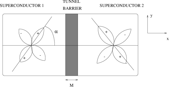
FIG. 1.: Structure considered in this paper. M is the matrix element linking superconductors 1 and 2. In case of d-wave, the pair potential in each superconductor varies with the direction $\theta$ according to $\Delta(\theta)=\Delta_{0}\cos(2\theta-2\alpha)$, where $\alpha$ is the angle that the main lobe makes with the x-axis.

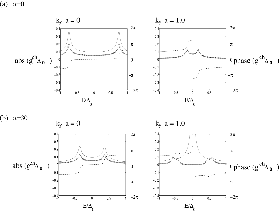
FIG. 2.: Magnitude and phase of the pair correlation function $g^{eh}$ at a surface for $\alpha=0$ degrees and 30 degrees with (i) $k_{y}a=0$ and (ii) $k_{y}a=1$. These correspond to (i) $\theta=0$ and (ii) $\theta=50$ degrees respectively, since $sin\theta=k_{y}/k_{f}$ and $k_{f}a=1.3$ . Also shown is the magnitude of the bulk pair correlation function. (—-:surface(magnitude), …..: surface(phase), xxx: bulk(magnitude) )

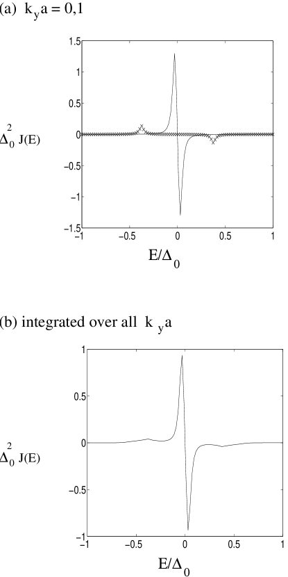
FIG. 3.: Josephson current spectrum for a d-wave junction having $\alpha_{1}=\alpha_{2}=30$ degrees (a) with $k_{y}a=0,1$ (xxx : $k_{y}a=0$, solid : $k_{y}a=1$) , (b) integrated over all values of $k_{y}a$.

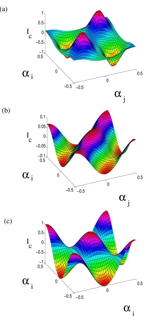
FIG. 4.: Critical current (normalized) of Josephson junctions as a function of the misalignment angles $\alpha_{1}$ and $\alpha_{2}$ (in units of $\pi$): (a) $kT=0$, (b) $kT=.5\Delta_{0}$ and (c) Phenomenological result based on $I_{c}=I_{c0}cos(2\alpha_{1})cos(2\alpha_{2})$

REFERENCES

- [1] M. Sigrist and T. M. Rice, Rev. Mod. Physics 67, 503 (1995); J. Phys. Soc. Jpn. 61, 4283, (1992).
- [2] See for example, C. R. Hu Phys. Rev. Lett. 72, 1526 (1994); S. Kashiwaya et. al. Phys. Rev. B51, 1350 (1995); J. H. Hu et. al. Phys. Rev. B53, 3604 (1996); M. Matsumoto and H. Shiba, J. Phys. Soc. Jpn. 64, 1703 (1995).
- [3] See for example, L. J. Buchholtz, M. Palumbo, D. Rainer and J. A. Sauls, J. Low Temp. Physics, 101, 1099 (1995); also 101, 1079 (1995).
- [4] I. I. Mazin, A. A. Golubov and A. D. Zaikin, Phys. Rev. Lett. 75, 2574 (1995); R. Combescot and X. Leyronas, Phys. Rev. Lett. 75, 3732 (1995).
- [5] D. J. Van Harlingen, Rev. Mod. Physics 67, 515 (1995) and references therein.
- [6] See for example, C. C. Tsuei et. al. Science 271, 329 (1996); J. R. Kirtley et.el. Nature 373, 225 (1995); D. A. Wollman, D. J. van Harlingen, C. W. Lee, D. M. Ginsberg and A. J. Leggett, Phys. Rev. Lett. 71 2134 (1993).
- [7] For a thorough review of the work on high- Josephson junctions see K. A. Delin and A. W. Kleinsasser, Superconductor Science and Technology 9, 227, (1996).
- [8] Eq 2 is valid for strong coupling too, if we use the correct pair correlation functions taking the coupling into account [10].
- [9] G. B. Arnold, J. Low Temp. Physics, 59, 143 (1985).
- [10] M. P. Samanta and S. Datta (unpublished).
- [11] V. Ambegaokar and A. Baratoff, Phys. Rev. Lett. 10, 486 (1963); 11, 104 (1963).
- [12] J. H. Xu, J. L. Shen, J. H. Miller Jr. and C. S. Ting, Phys. Rev. Lett., 73, 2492 (1994).
- [13] Note that in evaluating or we do not need to include in eq 10 any overall phase factor associated with the pair potential . Also, in general, .
- [14] Y. Tanaka and S. Kashiwaya, Phys. Rev. B 53, R11957 (1996).
- [15] We have not taken into account the dependence of M.
- [16] However, in this paper (and in ref [14]) only short clean junctions are considered. The mid-gap contribution may be suppressed for long or disordered junctions.