[

Bosonization in the two-channel Kondo model

Abstract

The bosonization of the $S=1/2$ anisotropic two-channel Kondo model is shown to yield two equivalent representations of the original problem. In a straight forward extension of the Emery-Kivelson approach, the interacting resonant level model previously derived by the Anderson-Yuval technique is obtained. In addition, however, a “($\sigma$,$\tau$)” description is also found. The strong coupling fixed point of the ($\sigma$,$\tau$) model was originally postulated to be related to the intermediate coupling fixed point of the two-channel Kondo model. The equivalence of the $\sigma$,$\tau$ model to the two-channel Kondo model is formally established. A summary of what one may learn from a simple study of these different representations is also given.

]

The physics of the isotropic two-channel Kondo problem has been the focus of intense theoretical investigation since it was first known to have an intermediate coupling fixed point[1]. The essential physics was understood at that time to be due to an overscreening of the impurity spin leaving a residual spin object to interact with the conduction electrons even in the strong coupling limit. This has since been clarified by the exact solution of the problem using the Bethe Ansatz[2, 3].

Considerable insight into this exact solution was recently provided by two apparently different approaches which both enable much of the physics of the problem to be extracted by elementary methods. In the first of these, Emery and Kivelson[4] found that a bosonized version of the model could be reduced to a resonant level model which becomes diagonal for a special value of perpendicular coupling $J_{z}$. The non-Fermi liquid thermodynamics and the Wilson ratio of $8/3$ found near this point[5] are consistent with the exact solution. In the second approach, Coleman et. al.[6] postulated a “$\sigma+\tau$” model, where an $S=1/2$ impurity interacts with both the spin ($\sigma$) and charge ($\tau$) degrees of freedom of a single channel of conduction electrons. This model has a strong–coupling fixed point which, the authors argue, is equivalent to the intermediate coupling fixed point of the symmetric two-channel Kondo problem. A strong coupling expansion about this fixed point also gives a good account of the low energy physics of the exact solution and again reproduces the correct Wilson ratio.

In analyzing the more general case where channel anisotropy in the couplings is allowed, a similar pattern of events has transpired. Andrei and Jerez[7] have obtained a solution for the thermodynamics of this model using the full machinery of the Bethe Ansatz. At the same time, an equivalent interacting resonant level model was obtained by Fabrizio et. al.[8] by the Anderson-Yuval technique and analyzed in the vicinity of the Toulouse point. The ($\sigma$,$\tau$) model was also extended by Coleman and Schofield[9] to examine the fixed point of that model away from the symmetric point by a duality transformation. Controversially, the authors argued that a Fermi liquid description of the strong coupling fixed point is not possible because of the Majorana structure of the Anderson model they derive at strong coupling. Up until now, the weak point in applying their argument to the two-channel Kondo model lies in the absence of the precise link between this model and the ($\sigma$,$\tau$) model which they treat. The need for such a connection has become all the more pressing following recent papers by Zhang and Hewson [10] which argue that the models have different fixed points on the basis of a comparison of the resistivities of the two models.

In this paper, I formally derive the ($\sigma,\tau$) description from the two-channel Kondo model using bosonization. The result is valid for both the channel symmetric and anisotropic cases. The resonant level model obtained by Fabrizio et. al. [8] is also derived by this method (a result undoubtedly known by the authors of that paper). This gives a foundation for understanding how these simple pictures relate to the exact solution. In particular the explicit mapping between the ($\sigma,\tau$) model and the two-channel Kondo model shows why the “resistivity” calculated by Zhang and Hewson [10] for the ($\sigma,\tau$) model has no correspondence with the two channel Kondo model. Recent work by Kotliar and Si[11] has emphasized the importance of “Klein” factors in finding Toulouse points so, for completeness, I give a precise account of the bosonization technique including these factors.

The two-channel Kondo problem describes how an impurity spin (taken here to be $S=1/2$) at the origin interacts with a conduction sea of spin–half electrons of two flavors (channels). Typically one restricts the interaction to being in the $s$-wave sector for each flavor reducing the problem to finding the radial wave functions of the conduction sea. By mapping the incoming partial waves onto the positive $x$ axis and out-going waves onto the negative $x$ axis one can treat the problem as left-moving 1D chiral electrons interacting with an impurity at the origin[12]

$${\cal H}={\cal H}_{0}+{\cal H}_{\perp}+{\cal H}_{\parallel}+{\cal H}_{B}\;,$$ (1)

where

$${\cal H}_{0} = \int_{-\infty}^{\infty}\!\!\!dx\;iv_{F}\psi_{\nu,\sigma}^{\dagger}(x){\partial\over\partial x}\psi_{\nu,\sigma}(x)\;,$$ (2)

$${\cal H}_{\perp} = \frac{1}{2}\left[J_{\perp}^{(\nu)}S^{+}\psi^{\dagger}_{\nu\downarrow}(0)\psi_{\nu\uparrow}(0)+{\rm H.c.}\right]\;,$$ (3)

$${\cal H}_{\parallel} = \frac{1}{2}J_{z}^{(\nu)}S_{z}\left[\psi^{\dagger}_{\nu\uparrow}(0)\psi_{\nu\uparrow}(0)-\psi^{\dagger}_{\nu\downarrow}(0)\psi_{\nu\downarrow}(0)\right]\;,$$ (4)

$${\cal H}_{B} = BS_{z}\!+\!\frac{B}{2}\!\!\int_{-\infty}^{\infty}\!\!\!\!\!\!\!dx\!\left[\psi^{\dagger}_{\nu\uparrow}(x)\psi_{\nu\uparrow}(x)-\psi^{\dagger}_{\nu\downarrow}(x)\psi_{\nu\downarrow}(x)\right]\!.$$ (5)

Summation is implicit over repeated channel indices $\nu=1,2$ and spin configurations $\sigma=\uparrow,\downarrow$. $S^{\pm}$ and $S_{z}$ define the $S=1/2$ spinor at the origin. I have explicitly included a coupling to an external magnetic field in ${\cal H}_{B}$ and allowed asymmetry in both spin space [e.g. $J^{(\nu)}_{\perp}\neq J_{z}^{(\nu)}$] and between channels [e.g. $J^{(1)}_{\perp}\neq J^{(2)}_{\perp}$].

I now proceed by bosonizing this model. This is a standard procedure which I briefly review for chiral fermions moving a ring of length $L$ with anti-periodic boundary conditions $\psi(L/2)=-\psi(-L/2)$ (ensuring that $k_{F}=0$ defines a unique ground state). Ultimately the limit $L\rightarrow\infty$ will be taken. As noted by Mattis and Lieb[13] particle-hole excitations of a chiral 1D model may be represented by bosonic variables

$$b^{\dagger}_{q}=\sqrt{2\pi\over Lq}\sum_{k}\!:\!c^{\dagger}_{k+q}c_{k}\!\!:,\quad b_{q}=\sqrt{2\pi\over Lq}\sum_{k}\!:\!c^{\dagger}_{k}c_{k+q}\!\!:.$$ (6)

These operators act on excitations above a vacuum state where all states below $k_{F}$ are occupied and all those above are empty. Normal ordering ‘::’ with respect to this vacuum is essential to avoid the infinities associated with the infinite number of occupied states. Here $q=2\pi n/L>0$. These bosons obey the correct commutation relations $[b_{k},b^{\dagger}_{q}]=\delta_{kq}$ by virtue of the absence of a lower bound on the occupied momentum states. The electron creation operators are defined such that $\psi^{\dagger}(x)=L^{-1/2}\sum_{k}e^{ikx}c^{\dagger}_{k}$.

The idea behind bosonization is to use these bosons as an alternative to the fermion basis for describing 1D models. The requirement that this new basis be complete means that, in addition to the bosons which describe particle-hole excitations, we also need ladder operators which create extra particles of a given spin and flavor in the Fermi sea[14], $F^{\dagger}_{i}$. These ladder operators (or “Klein factors”) must also anticommute between different electron flavors and spins to reflect the fermionic nature of the underlying particles created. They may also be defined to be unitary. There are many possible representations for the ladder operators, and I chose to represent $F^{\dagger}_{i}$ by $(-1)^{\sum_{j<i}\hat{N}_{j}}e^{i\hat{\theta}_{i}}$. Here the Hermitian operator $\hat{\theta}_{i}$ is conjugate to the number operator $\hat{N}_{i}$: $[\hat{\theta}_{i},\hat{N}_{j}]=i\delta_{ij}$ and $[\hat{\theta}_{i},\hat{\theta}_{j}]=0$. This formulation corresponds to a particular ordering of the vacuum by the arbitrary assigning of an order to the spin/flavor degree of freedom $i$ (e.g. $1,\uparrow$ comes before $2,\downarrow$). By ensuring that the ladder operators commute with boson fields, Haldane was able to show that one may represent a Fermi field as

$$\psi_{i}^{\dagger}(x)=\lim_{\alpha\rightarrow 0}{e^{ik_{F}x}\over\sqrt{2\pi\alpha}}(-1)^{\sum_{j<i}\hat{N}_{j}}e^{i\Phi_{i}(x)}\;,$$ (7)

where

$$\Phi_{i}(x)=\hat{\theta}_{i}+{2\pi x\hat{N}_{i}\over L}+i\sum_{q>0}\!\sqrt{2\pi\over Lq}\!\left[e^{-iqx-q\alpha/2}b_{i,q}-{\rm H.c.}\right]\!.$$ (8)

($\alpha$ is a short wavelength cut-off which regularizes the momentum sums.) Together with Eq. 7, the following relations form a dictionary for bosonization

$$\left[\Phi(x)_{i},\Phi_{j}(y)\right] = -i\delta_{ij}\pi{\rm sgn}(x-y)\;,$$ (9)

$$\partial_{x}\Phi(x)=\Phi^{\prime}(x) = 2\pi:\psi^{\dagger}(x)\psi(x):\;,$$ (10)

$$\left[\Phi^{\prime}(x),\Phi(y)\right] = -2\pi i\delta(x-y)\;,$$ (11)

$$iv_{F}\int_{-L/2}^{L/2}\!\!\!\!dx\;\psi^{\dagger}{\partial\over\partial x}\psi = {v_{F}\over 4\pi}\int_{-L/2}^{L/2}:\left[\Phi^{\prime}(x)\right]^{2}:dx\;.$$ (12)

Using this dictionary, I now express the Hamiltonian of Eq. 1 in terms of phase fields for each species of fermion. I choose $\{1\uparrow,2\downarrow,1\downarrow,2\uparrow\}$ as my ordering convention for the Klein factors. Any ordering will work, but this one simplifies the computation as will be explained later. Following both Emery and Kivelson and Sengupta and Georges, the spin and charge degrees of freedom can be separated and both have symmetric and antisymmetric combinations across the two channels:

$$\Phi_{c_{\pm}} = {1\over 2}\left[\left(\Phi_{1\uparrow}+\Phi_{1\downarrow}\right)\pm\left(\Phi_{2\uparrow}+\Phi_{2\downarrow}\right)\right]\;,$$ (13)

$$\Phi_{s_{\pm}} = {1\over 2}\left[\left(\Phi_{1\uparrow}-\Phi_{1\downarrow}\right)\pm\left(\Phi_{2\uparrow}-\Phi_{2\downarrow}\right)\right]\;.$$ (14)

The number operators are defined analogously.

In terms of this decoupling, the Hamiltonian may be written as

$${\cal H}_{0}={v_{F}\over 4\pi}\sum_{\lambda=\{c_{\pm},s_{\pm}\}}\int_{-\infty}^{\infty}:\left[\Phi^{\prime}_{\lambda}(x)\right]^{2}:dx\;,\qquad\qquad$$ (15)

$${\cal H}_{\perp}={J_{\perp}^{(1)}\over 4\pi\alpha}(-1)^{\hat{N}_{c_{+}}\!+\hat{N}_{s_{-}}}\!\!\left\{\!S^{+}e^{-i\left[\Phi_{s_{+}}(0)+\Phi_{s_{-}}(0)\right]}-{\rm H.c.}\right\}{}$$ (17)

$${}-\!{J_{\perp}^{(2)}\over 4\pi\alpha}(-1)^{\hat{N}_{c_{-}}\!\!-\hat{N}_{s_{-}}}\!\!\left\{\!S^{+}e^{-i\left[\Phi_{s_{+}}(0)-\Phi_{s_{-}}(0)\right]}-{\rm H.c.}\right\},$$

$${\cal H}_{\parallel} = {J_{z}^{(1)}\!+J_{z}^{(2)}\over 4\pi}S_{z}\Phi^{\prime}_{s_{+}}(0)+{J_{z}^{(1)}\!-J_{z}^{(2)}\over 4\pi}S_{z}\Phi^{\prime}_{s_{-}}(0),$$ (18)

$${\cal H}_{B} = B\left[S_{z}+{1\over 4\pi}\int_{-\infty}^{\infty}\Phi^{\prime}_{s_{+}}(x)dx\right]\;.$$ (19)

From this Hamiltonian, I will first derive the interacting resonant level model obtained by Fabrizio et. al.[8]. I will then show the connection to the ($\sigma,\tau$) model.

The resonant level model is obtained by the unitary transformation used by Emery and Kivelson

$$U=e^{-i\sigma_{z}\Phi_{s_{+}}(0)/2}\;,$$ (20)

where $\sigma_{z}$ is the 3rd Pauli spin matrix. The advantage of my original choice of ordering is that, since $(-1)^{N_{s_{+}}}$ does not appear, this transformation does not affect the Klein factors.

Using Eq. 11 and the fact that, if $[A,B]$ commutes with both $A$ and $B$, then $[e^{\lambda A},B]=\lambda[A,B]e^{\lambda A}$, I find

$$U^{\dagger}\Phi^{\prime}_{s+}(x)U=\Phi^{\prime}_{s+}(x)-2\pi S_{z}\delta(x)\;.$$ (21)

With ${\cal H^{\prime}}=U^{\dagger}{\cal H}U$ I have, ${\cal H}_{0}^{\prime}={\cal H}_{0}$ and

$${\cal H}^{\prime}_{\perp} = {J_{\perp}^{(1)}\over 4\pi\alpha}(-1)^{\hat{N}_{c_{+}}+\hat{N}_{s_{-}}}\left[S^{+}e^{-i\Phi_{s_{-}}(0)}-{\rm H.c.}\right]$$ (23)

$$+{J_{\perp}^{(2)}\over 4\pi\alpha}(-1)^{\hat{N}_{c_{-}}-\hat{N}_{s_{-}}}\left[S^{+}e^{i\Phi_{s_{-}}(0)}-{\rm H.c.}\right],$$

$${\cal H^{\prime}}_{\parallel} = \left(\bar{J}_{z}-2\pi v_{F}\right){S_{z}\over 2\pi}\Phi^{\prime}_{s_{+}}(0)+\delta J_{z}{S_{z}\over 2\pi}\Phi^{\prime}_{s_{-}}(0)\;,$$ (24)

$${\cal H}^{\prime}_{B} = {B\over 4\pi}\int_{-\infty}^{\infty}\Phi^{\prime}_{s_{+}}(x)dx\;.$$ (25)

Here I have written $\bar{J}_{z}=(J_{z}^{(1)}+J_{z}^{(2)})/2$, $\delta J_{z}=(J_{z}^{(1)}-J_{z}^{(2)})/2$ and will similarly define $\bar{J}_{\perp}$ and $\delta J_{\perp}$.

To obtain the equivalent resonant level model I ‘refermionize’ the problem by expressing the boson fields $\Phi_{\lambda}$ in terms of fermion fields $\psi_{\lambda}$. For example,

$$\begin{array}[]{cc}\psi^{\dagger}_{s_{-}}={e^{i\Phi_{s_{-}}(x)}\over\sqrt{2\pi\alpha}}\;,&\psi^{\dagger}_{s_{+}}={(-1)^{\hat{N}_{s_{-}}}e^{i\Phi_{s_{+}}}\over\sqrt{2\pi\alpha}}\;.\\ \end{array}$$ (26)

(Again the ordering of these fermions is arbitrary.) Notice that since there are no terms in the Hamiltonian which change $N_{c_{\pm}}$, the operators $(-1)^{\hat{N}_{c_{\pm}}}$ simply fix an arbitrary sign for $J_{\perp}^{(1),(2)}$. Also note that for $S=1/2$, I can define $S^{+}(-1)^{\hat{N}_{s_{-}}}=d^{\dagger}$, where $d^{\dagger}$ creates a fermion which anticommutes with $\psi^{\dagger}_{s_{-}}$. (Maintaining the Klein factors is crucial to obtaining this relation.)

Thus finally I may write the equivalent resonant level model for the two-channel anisotropic Kondo model as

$${\cal H} =iv_{F}\int_{-\infty}^{\infty}\left[\sum_{\lambda}\psi^{\dagger}_{\lambda}{\partial\over\partial x}\psi_{\lambda}+B\psi^{\dagger}_{s_{+}}\psi_{s_{+}}\right]dx$$ (29)

$$+{\bar{J}_{\perp}\over 2i\sqrt{\pi\alpha}}\hat{b}\left[\psi^{\dagger}_{s_{-}}+\psi_{s_{-}}\right]_{x=0}+{\delta J_{\perp}\over 2\sqrt{\pi\alpha}}\hat{a}\left[\psi^{\dagger}_{s_{-}}-\psi_{s_{-}}\right]_{x=0}$$

$$+i\hat{a}\hat{b}\left[\left(\bar{J}_{z}-2\pi v_{F}\right)\psi^{\dagger}_{s_{+}}\psi_{s_{+}}+\delta J_{z}\psi^{\dagger}_{s_{-}}\psi_{s_{-}}\right]_{x=0}.$$

The complex fermion $d$ has been expressed in terms of its real and imaginary (i.e. Majorana) components $\hat{a}=(d^{\dagger}+d)/\sqrt{2}$ and $\hat{b}=(d^{\dagger}-d)/i\sqrt{2}$. This emphasizes that the Majorana representation for the spin is perhaps the most natural since the conduction sea is seen to interact independently with the spin via its Majorana components. This is the model obtained by Fabrizio et. al.[8] using the Anderson–Yuval technique—essentially identifying the perturbation expansions of the two models [16]. The charge degrees of freedom ($\lambda=c_{\pm}$) have completely decoupled and remain free—an observation that will be exploited in the second part of the paper. The Toulouse point corresponds to $\bar{J}_{z}=2\pi v_{F}$ and $\delta J_{z}=0$ where the model is non interacting and may be solved exactly[15]. Here the impurity spin completely decouples from the magnetic field so the local spin susceptibility is zero. The constraint $\delta J_{z}=0$ means that in the Toulouse point only describes the region in the vicinity of the symmetric model.

This model was analyzed in full in Ref. [8] for the region around the Toulouse point. The two resonant level widths $\Delta_{b}=\bar{J}_{\perp}^{2}/4\pi v_{F}\alpha$ and $\Delta_{a}=(\delta J_{\perp})^{2}/4\pi v_{F}\alpha$, associated with the two independent Majorana modes, represent the two relevant energy scales of the problem.

A second equivalent description of the problem is obtained rather straightforwardly from the Hamiltonian expressed in terms of spin and charge degrees of freedom Eq. 15–19. Refermionizing this Hamiltonian using Eq. 26, one obtains

$${\cal H} =iv_{F}\sum_{\lambda}\int_{-\infty}^{\infty}\!\!\!\!dx\psi^{\dagger}_{\lambda}{\partial\over\partial x}\psi_{\lambda}+B\!\left[S_{z}+{1\over 2}\int_{-\infty}^{\infty}\!\!\!\!\!\!\!:\rho_{s_{+}}(x):dx\right]$$ (32)

$$+{J_{\perp}^{(1)}\over 2}\left[S^{+}\psi_{s_{-}}\psi_{s_{+}}+{\rm H.c.}\right]+{J_{\perp}^{(2)}\over 2}\left[S^{+}\psi^{\dagger}_{s_{-}}\psi_{s_{+}}+{\rm H.c.}\right]$$

$$+{J_{z}^{(1)}\over 2}:\!\left[\rho_{s_{+}}(0)+\rho_{s_{-}}(0)\right]\!:+{J_{z}^{(2)}\over 2}:\!\left[\rho_{s_{+}}(0)-\rho_{s_{-}}(0)\right]\!:.$$

The normal ordering of the density operators is an instruction to subtract off the contribution coming from the vacuum state. The mean occupancy in the vacuum at $x=0$ is $1/2$ for any fermion so I may replace $:\!\rho(x)\!:$ by $\rho(x)-1/2$. The ($\sigma$,$\tau$) description is apparent if I re-label subscripts $s$ and $c$ as channel indices 1 and 2, and subscripts $+$ and $-$ as $\uparrow$ and $\downarrow$. This relabeling is shown pictorially in Fig. 1. I may then write the Hamiltonian, here for the rotationally invariant case, $J_{\perp}=J_{z}$, as

$${\cal H} = {\cal H}_{0}+\left[J^{(2)}\vec{\sigma}_{1}(0)+J^{(1)}\vec{\tau}_{1}(0)\right]\cdot\vec{S}$$ (34)

$$+\vec{B}\cdot\left[\vec{S}+\int_{-\infty}^{\infty}\vec{\sigma}_{1}(x)+\vec{\tau}_{1}(x)dx\right]\;,$$

where

$$\vec{\sigma_{i}} = (\psi^{\dagger}_{i\uparrow},\ \psi^{\dagger}_{i\downarrow})\cdot{\vec{\sigma}\over 2}\cdot\left(\begin{array}[]{c}\psi_{i\uparrow}\\ \psi_{i\downarrow}\end{array}\right)\;,$$ (37)

$$\vec{\tau}_{i} = (\psi^{\dagger}_{i\uparrow},\;\psi_{i\downarrow})\cdot{\vec{\sigma}\over 2}\cdot\left(\begin{array}[]{c}\psi_{i\uparrow}\\ \psi^{\dagger}_{i\downarrow}\end{array}\right)\;.$$ (40)

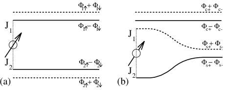
FIG. 1.: A pictorial representation of the relationship between the two-channel Kondo model (a) and the $(\sigma,\tau)$ model (b). By expressing the boson fields $\Phi$ in terms of spin and charge degrees of freedom $(s_{\pm},c_{\pm})$ instead of the original flavor and spin decoupling $(1_{\uparrow,\downarrow},2_{\uparrow,\downarrow})$ I can refermionize the model to obtain the $(\sigma,\tau)$ formulation.

This is precisely the model treated in Ref. [6] for the symmetric case [$J^{(1)}=J^{(2)}$] and in Ref. [9] in the general case [$J^{(1)}\neq J^{(2)}$]. The impurity is seen to interact now with the spin and charge degrees of freedom of a single chain leaving a second chain—representing what were previously charge excitations—decoupled from the spin (see Fig. 1). Since both the ($\sigma,\tau$) description and the interacting resonant level models can be derived from the original Kondo problem, they are both equivalent representations of the model. Thus, for example, the low energy spectrum of the $(\sigma,\tau)$ model plus the uncoupled chain will be identical to that of the two channel Kondo model. What then are the relative merits of these two equivalent models over the original formulation?

By studying the non-interacting Toulouse point of the resonant level description a qualitative picture of the thermodynamics may be obtained. One sees a two-stage quenching of the entropy of the impurity spin as the temperature is lowered through the two energy scales. At temperatures between these two energy scales the thermodynamic response is controlled by the fixed point of the channel symmetric case. For example, the local spin susceptibility is logarithmically divergent as a function of temperature. At low temperatures the specific heat and susceptibility revert to their Fermi liquid forms. These results mirror those obtained from the exact solution. However, the disadvantage of this approach is that to solve the model one is restricted to the region near $J_{z}^{(1)}=J_{z}^{(2)}\gg J_{\perp}$ and so one may fail to identify properties which are universal functions of the energy scales. For example, the Wilson ratio is vanishingly small near the Toulouse points in contrast to the rotationally invariant case where the Wilson ratio spans the range $(0,2]$.

It is in understanding the low temperature fixed point behavior that the ($\sigma,\tau$) description excels. Unlike the original formulation, the strong coupling fixed point of the ($\sigma,\tau$) model is stable: over-screening of the impurity spin is prevented by the Pauli principle. The intermediate coupling fixed point of the two-channel Kondo model has beenmoved to infinity by the transformation to the ($\sigma,\tau$) picture. One may then exploit a strong coupling expansion to examine the physics near the fixed point. Just as in the single channel case [17, 18], symmetries restrict the form of the resulting fixed point Hamiltonian. As well as enabling a direct calculation of the Wilson ratio, one also obtains the form of the low-energy Hamiltonian. The Majorana character of this Hamiltonian is the basis for the conjecture that the excitations are not compatible with weakly interacting fermion quasi-particles [9].

Finally I address the issue of how one uses the fixed point Hamiltonian of the $(\sigma,\tau)$ model to compute the resistivity in the two-channel Kondo model. The two models are equivalent as we have shown but the mapping between them is linear only in the bosonized language of Eq. 14. Put simply, the electrons in the two-channel Kondo model are not the same electrons appearing in the $(\sigma,\tau)$ model. To calculate the resistivity of the two-channel Kondo model one must show how the electron Green’s function transforms under this mapping. It does not transform into the electron Green’s function in the $(\sigma,\tau)$ model as implicitly assumed in Ref. [10]. The appropriate correlator is expressible only in terms of the boson fields: for example

$${\cal G}_{1,\uparrow}(x_{1},x_{2};\tau)={\cal T}_{\tau}\langle\psi_{1,\uparrow}(x_{2},\tau)\psi^{\dagger}_{1,\uparrow}(x_{1},0)\rangle,\quad\quad$$ (41)

$$\rightarrow\sim{1\over 2\pi\alpha}{\cal T}_{\tau}\langle:\!e^{-i\sum_{\lambda}\Phi_{\lambda}(x_{2},\tau)/2}::\!e^{i\sum_{\lambda}\Phi_{\lambda}(x_{1},0)/2}:\rangle\;,$$ (42)

where $\lambda=\{c_{\pm},s_{\pm}\}$. Following Affleck and Ludwig [19], the low temperature resistivity in the isotropic two-channel Kondo model is found by considering this correlator with $x_{2}<0<x_{1}$ in the fixed point Hamiltonian of Ref. [6]. The leading temperature dependence comes from consideration of the leading irrelevant operator which affects this correlator at first order and, since it has dimension $1/2$, leads to a $T^{1/2}$ correction [20].

In conclusion, two methods have been proposed recently to give a simple account of the physics of the two-channel Kondo model both at and away from the channel symmetric point. These methods sidestep, at the expense of completeness, the full formalism of the Bethe Ansatz by considering models related to the original two-channel Kondo problem. In this paper these related models are formally derived from the original two-channel Kondo model via bosonization. In describing the bosonization technique, care is taken to include explicitly the Klein factors which preserve the anticommutation relations between the fermions on different channels. As expected, the interacting resonant level model found previously by Fabrizio et. al. is found as a simple generalization of the Emery-Kivelson Hamiltonian. In addition, however, the ($\sigma,\tau$) model with its strong coupling fixed point is also obtained directly from the two-channel Kondo model by bosonization. This establishes the equivalence of this model to the original two channel Kondo model. The relative merits of these two approaches are discussed.

During the course of this work I have benefitted enormously from discussions with N. Andrei, P. Azaria, P. Coleman, A. Jerez, G. Kotliar, Ph. Nozières, A. Sengupta and Q. Si. I also gratefully acknowledge the financial support of a Royal Society (NATO) travel fellowship and NSF grants DMR93–12138 and DMR92–21907.

REFERENCES

- [1] Ph. Nozières and A. Blandin, J. Phys. (Paris) 41, 193 (1980).
- [2] N. Andrei and C. Destri, Phys. Rev. Lett. 52, 364 (1984).
- [3] A. M. Tsvelik and P. B. Wiegmann, Z. Phys. B 54, 201 (1984).
- [4] V. J. Emery and S. Kivelson, Phys. Rev. B 46, 10812 (1992).
- [5] A. M. Sengupta and A. Georges, Phys. Rev. B 49, 10020 (1994).
- [6] P. Coleman, L. B. Ioffe and A. M. Tsvelik, Phys. Rev. B 52, 6611 (1995).
- [7] N. Andrei and A. Jerez, Phys. Rev. Lett. 74, 4507 (1995).
- [8] M. Fabrizio, A. Gogolin and Ph. Nozières, Phys. Rev. Lett. 74, 4503 (1995): Phys. Rev. B 51, 16088 (1995).
- [9] P. Coleman and A. J. Schofield, Phys. Rev. Lett. 75, 2184 (1995).
- [10] G.-M. Zhang and A. C. Hewson, Phys. Rev. Lett. 76, 2137 (1996).
- [11] G. Kotliar and Q. Si, preprint cond-mat/9508112.
- [12] I. Affleck and A. W. W. Ludwig, Nucl Phys. B 352, 849 (1991); 360. 641 (1991).
- [13] D. C. Mattis and E. H. Lieb, J. Math. Phys. 6, 304 (1963).
- [14] F. D. M. Haldane, J. Phys. C: Solid State Phys. 14, 2585 (1981).
- [15] G. Toulouse, Phys. Rev. B 46, 10812 (1970).
- [16] At first sight, the coefficients obtained in Ref. [8] differ from those obtained here. However this difference is an artifact of the regularization scheme [see F. Guinea, V. Hakim and A. Muramatsu, Phys. Rev. B 32, 4410 (1985) and references therein]. In bosonizing as above, a scattering phase shift is related to the scattering potential by in contrast to of the X-ray edge problem. Thus by expressing Eq. 29 in terms of the physical phase shifts I obtain the same coefficients as in Ref. [8]. For example, the Toulouse point here (, ) expressed in phase shifts implies , . I am grateful to Qimiao Si for drawing my attention to this point.
- [17] Ph. Nozières, J. Low Temp. Phys. 17, 31 (1974).
- [18] A. C. Hewson, Phys. Rev. Lett. 70, 4007 (1993).
- [19] I. Affleck and A. W. W. Ludwig, Phys. Rev. B 48 7292 (1993).
- [20] A. J. Schofield and A. Sengupta, in preparation.