Fictitious level dynamics: a novel approach to spectral statistics in disordered conductors

Abstract

We establish a new approach to calculating spectral statistics in disordered conductors, by considering how energy levels move in response to changes in the impurity potential. We use this fictitious dynamics to calculate the spectral form factor in two ways. First, describing the dynamics using a Fokker-Planck equation, we make a physically motivated decoupling, obtaining the spectral correlations in terms of the quantum return probability. Second, from an identity which we derive between two- and three-particle correlation functions, we make a mathematically controlled decoupling to obtain the same result. We also calculate weak localization corrections to this result, and show for two dimensional systems (which are of most interest) that corrections vanish to three-loop order.

I Introduction

Numerous properties of quantum systems can be described in terms of their energy spectra. For complex systems an exact determination of energy levels is not feasible, and a statistical description becomes necessary. It turns out that the Wigner-Dyson (WD) statistics [1, 2] of eigenvalues of random Hermitian matrices describes energy levels in a wide variety of different systems [3]. The joint distribution of eigenvalues is dominated by level repulsion and is universal in the sense that level correlations depend only upon the symmetry of the Hamiltonian while all specific properties of the system are absorbed into the mean level spacing, $\Delta$. A very important feature of WD statistics is that – by construction of invariant ensembles of random matrices – spectral properties are independent of eigenstate correlations. In real systems such an independence can at best be approximate. It holds, however, in the ergodic regime where the entire phase space of a system is explored. If a non-ergodic regime is of interest, not only is WD statistics inapplicable but the whole concept of the independence of spectral and eigenstate correlations should be re-examined.

Disordered mesoscopic conductors present a natural ensemble for a statistical description - the ensemble of impurity configurations. In this case spectral statistics in the non-ergodic regime are very important for both transport and thermodynamic properties of electrons. Different regimes in disordered conductors are determined by the energy or time scale, as shown in Fig. 1. The ergodic regime involves energy level separations $\varepsilon\lesssim E_{c}\equiv\hbar/t_{\text{erg}}$ where $E_{c}$ is called the Thouless energy, and $t_{\text{erg}}\sim D/L^{2}$ is the time required for the electronic diffusive motion, with diffusion constant $D$, to fill all phase space, in a sample of size $L$. The quantum limit of this regime corresponds to smaller energy separations, $\varepsilon\lesssim\Delta$, where $\Delta$ is the mean level spacing, and to longer times $t\gtrsim t_{\!{}_{H}}$, where $t_{\!{}_{H}}\equiv\hbar/\Delta$ is the Heisenberg time. Note that the ratio $E_{c}/\Delta$ is proportional to the dimensionless conductance $g$ (i.e. the conductance measured in the units of $e^{2}/\hbar$), and is large in the metallic phase. The diffusive regime involves energies $\hbar/t_{\text{erg}}\lesssim\varepsilon\lesssim\hbar/t_{\text{el}}$, where $t_{\text{el}}$ is mean elastic-scattering time. The largest energies, $\hbar/t_{\text{el}}\lesssim\varepsilon\lesssim\varepsilon_{\!{}_{F}}$, (where $\varepsilon_{\!{}_{F}}$ is the Fermi energy) and the shortest times, $t\lesssim t_{\text{el}}$, correspond to the ballistic regime in which multiple scattering by impurities is irrelevant.

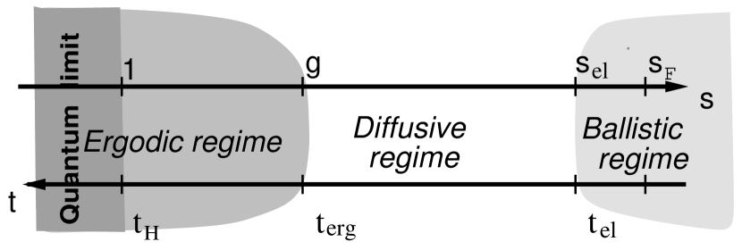
FIG. 1.: Regimes of energy and time in a disordered metal; here $s_{\text{el}}=\hbar/t_{\text{el}}\Delta$ and $s_{\!{}_{F}}=\varepsilon_{\!{}_{F}}/\Delta$.

It was first conjectured by Gor’kov and Eliashberg [4] and then shown by Efetov [5] that spectral correlations in the ergodic regime are described by the random matrix theory (RMT) of Wigner and Dyson. Correlations in the non-ergodic diffusive regime which are important, in particular, for universal conductance fluctuations were analysed by Altshuler and Shklovskii [6] at leading order in diagrammatic perturbation theory. Their results were later reproduced by Argaman et al [7] within the semiclassical approach, using the diagonal approximation.

We have recently developed [8] an alternative approach to level statistics in the non-ergodic regime which takes into account the inevitable coupling between eigenvalue and eigenstate correlations, and can be extended beyond the region of validity of the perturbative technique. Our approach is based on the idea of parametric motion through the ensemble of disordered Hamiltonians: we treat the energy eigenvalues as particles with fictitious dynamics induced by changing some parameter of the Hamiltonian. This dynamics takes the form of Brownian motion in a fictitious time $\tau$ related to the parameter being changed. Originally, this idea was employed by Dyson [9] in the context of RMT. Later, in the context of the semiclassical description, Pechukas [10] used motion along a smooth path in the space of Hamiltonians to generate fictitious dynamics of a different kind. Both Dyson and Pechukas were interested in level dynamics primarily as a way of generating the level distribution. By contrast, a number of recent authors [11], notably Szafer, Simons and Altshuler [12, 13], have investigated the dynamical problem in its own right, calculating parametric statistics: eigenvalue correlations as a function of position in the space of Hamiltonians. In distinction to our approach, eigenfunction correlations have played no role in previous work [11, 12, 13, 15, 16], an assumption justified only for the ergodic regime.

We have found [8] that a treatment based on Brownian motion through the ensemble of Hamiltonians provides a unified description of all regimes in disordered conductors, except the quantum limit ($t\gtrsim t_{\!{}_{H}}$, or $E\lesssim\Delta$), which is also beyond the scope of diagrammatic and semiclassical approaches. The main result is a new relation explicitly linking the spectral correlation function to the quantum return probability for an expanding wavepacket which, in turn, is related to a certain eigenfuction correlator. The derivation given in Ref [8] has a limitation: when obtaining a closed Langevin equation describing the Brownian motion, we make use of an uncontrolled, although physically transparent assumption. Thus, within the framework of that calculation it is not possible to establish exactly the region of validity and accuracy.

In this paper, we re-derive the relation between spectral and eigenstate correlation functions using a more explicit procedure: we decouple a certain exact relation between two- and three-level correlation functions using the Kirkwood superposition approximation. Then we examine the accuracy of this decoupling using perturbative diagrammatic techniques. Remarkably, it not only reproduces the results of the diagonal approximation [6, 7], but holds well beyond it. We show this to third order in a perturbative expansion in $g^{-1}$, for two-dimensional systems with or without time-reversal symmetry. We are therefore encouraged to believe that the connection between spectral and eigenstate correlation functions should be useful rather generally, and especially for problems where the usual diagrammatic technique cannot straightforwardly be applied, such as spectral statistics in the critical regime near the Anderson transition.

II Definitions and main results

A convenient way to consider spectral correlations is to introduce fictitious level dynamics in response to changing some parameter $\lambda$ of the Hamiltonian. Thus we parameterize the ensemble of Hamiltonians as follows

$$H(\lambda) = H_{0}+\lambda W(\mathchoice{{\hbox{\boldmath$\displaystyle r$}}}{{\hbox{\boldmath$\textstyle r$}}}{{\hbox{\boldmath$\scriptstyle r$}}}{{\hbox{\boldmath$\scriptscriptstyle r$}}})\,.$$ (1)

Here both $H_{0}$ and $H(\lambda)$ belong to the same symmetry class, and the point $\lambda=0$ corresponds to some arbitrary choice of one of the many members of the same ensemble. We will specify the choice of $H_{0}$ and $W$ in the next section.

We consider in this paper the two-level correlation function (TLCF) and its Fourier transform, the spectral form factor, in a disordered conductor described by the Hamiltonian Eq. (1). Let $E_{n}(\lambda)$ be the energy levels of $H(\lambda)$. We introduce the density of states per unit volume (DoS) as

$$\rho(E,\lambda)={1\over L^{d}}\sum_{n}\delta\bigl{(}E-E_{n}(\lambda)\bigr{)}\,.$$ (2)

The mean level spacing, $\Delta$, is then related to the mean DoS, $\rho\equiv\langle\rho\rangle$, by $\Delta\!=\!(\rho L^{d})^{-1}$. The TLCF is defined as

$$R(s,\lambda)=\rho^{-2}\Bigl{<}\rho(E+s\Delta,\lambda)\rho(E,0)\Bigr{>}-1\,,$$ (3)

where $\omega=s\Delta$ is the energy difference between two levels. The mean DoS is practically a constant in the entire energy region of interest (as it changes only at scale of order $\varepsilon_{\!{}_{F}}$ while we consider energy windows centered at $\varepsilon_{\!{}_{F}}$ of width not exceeding $\hbar/t_{\text{el}}\ll\varepsilon_{\!{}_{F}}$). We consider only values of $\lambda$ small enough so that the statistical regime does not change and neither does the mean DoS (for large enough $L$ this nevertheless allows arbitrarily large $\lambda$ on the scale relevant for parametric correlations). Because of this the TLCF cannot depend on either $E$, or on the choice of the point $H_{0}$ in the ensemble (1). We define the (dimensionless) spectral form factor as

$$K(t,\lambda)=\int_{-\infty}^{\infty}e^{-ist/t_{\!{}_{H}}}R(s,\lambda)\,ds\,.$$ (4)

Our main result relates the spectral form factor to the quantum return probability $p(t)$ of a diffusing electron as follows:

$$K(t)={(2\pi\hbar\rho)^{-1}|t|\,p(t)\over{1+(\pi\hbar\rho)^{-1}\int_{0^{+}}^{|t|}\,p(t^{\prime})dt^{\prime}}}\,.$$ (5)

We have obtained this expression for times shorter than the Heisenberg time $t_{\!{}_{H}}\equiv\hbar/\Delta$. Here we define $p(t)$ as the probability density for the wave packet, originally created in a small volume $V_{0}\sim\ell^{d}$, to remain in this volume at the time $t$ ($\ell$ is the elastic mean free path which is a natural coarse-graining size for the disordered metal; however, we could choose $V_{0}$ arbitrarily, provided that $\ell^{d}\gtrsim V_{0}\gtrsim\lambda_{\!{}_{F}}^{d}$ where $\lambda_{\!{}_{F}}$ is the Fermi wavelength). The ensemble-averaged return probability is related, as we will show later, to the following wave-function correlations:

$$p(t) = \int\!\!d^{d}r\,\left<\sum_{l}|\psi_{n}(r)|^{2}|\psi_{n+l}(r)|^{2}e^{-i(E_{n}-E_{n+l})t/\hbar}\right>\,.$$ (6)

It is important to note that, by definition of the wave packet above, the summation here is limited to the number of levels ${\cal N}\sim L^{d}/V_{0}$ with energies lying within the energy band of width $E_{0}\sim 1/\rho V_{0}$.

Equation (5) relates the spectral and wave-function correlations. Let us analyse this relation in the metallic phase. In the diffusive regime, $t_{\text{el}}\lesssim t\lesssim t_{\text{erg}}$, the quantum return probability $p(t)$ reduces at leading order to the classical return probability for random walks, multiplied by a symmetry factor $2/\beta$, where $\beta=1,\,2\,\text{or}\,4$ is the usual index corresponding to the orthogonal, unitary, and symplectic symmetry ensembles, respectively [3]:

$$p_{0}(t)={2\over\beta(4\pi Dt)^{d/2}}\,.$$ (7)

Noting that in the ballistic regime, $t\lesssim t_{\text{el}}$, $p(t)$ saturates at $p_{0}(t_{\text{el}})\sim 1/\ell^{d}$, one sees that the integral in the denominator of Eq. (5) is of order $(t_{\text{el}}\Delta/\hbar)(L/\ell)^{d}\sim g_{0}^{-1}$ for $d>2$, and of order $g_{0}^{-1}\ln(t/t_{\text{el}})$ for $d=2$. It is well known that such an integral describes a weak localization correction to conductance and other physical quantities[17, 18]. On the other hand, the quantum return probability $p(t)$ contains weak localization corrections itself. Neglecting these corrections in both the numerator and denominator of Eq. (5), we reduce it to

$$K_{0}(t) = (2\pi\hbar\rho)^{-1}|t|\,p_{0}(t)\,.$$ (8)

To leading order, this expression is also valid in the ergodic regime, $t_{\text{erg}}\lesssim t\ll t_{\!{}_{H}}$, where the classical return probability saturates at $(2/\beta)L^{d}$ so that the second term in the denominator in Eq. (5) is of order $t/t_{\!{}_{H}}\ll 1$ and may be neglected. We should not expect Eq. (5) to be correct in the quantum limit, $t\gg t_{\!{}_{H}}$, as we have derived it under the assumption that the opposite inequality holds, as will be seen later. Indeed, in this regime Eq. (5) gives the saturation of $K(t)$ at $1/2$ instead of the correct limiting value $K(t)=1$.

Equation (8) coincides with the result obtained by Argaman et al [7], using the diagonal approximation in semiclassical periodic-orbit theory. The Fourier transform of this expression corresponds to the TLCF obtained originally by Altshuler and Shklovskii[6]. In the diffusive regime, $R(s,0)\sim A_{d}\,g^{-d/2}s^{d/2-2}$, where $A_{d}$ is a numerical coefficient which is zero for $d\!=\!2$[19], and in the ergodic regime, $R(s,0)\sim-1/s^{2}$ [20].

The second relation we obtain between $K(t)$ and $p(t)$ is:

$$K(t)+(\pi\hbar\rho)^{-1}\int_{0+}^{|t|}K(t-t^{\prime})p(t^{\prime})dt^{\prime}=(2\pi\hbar\rho)^{-1}|t|p(t)$$ (9)

which we can see is very similar to Eq. (5). The latter is obtained from a diagrammatic analysis discussed in section (VI). The new feature is that we have a convolution of $K(t)$ and $p(t)$ which occurs because the decoupling is in $\omega$-space rather than $t$-space. In 2d, up to 3-loop order in perturbation theory, both these relations correctly reproduce the TLCF. It seems to us quite remarkable that a relation derived from a phenomenological model of energy level dynamics could be exact to 3-loop order. We note that the 2d case is expected to be a good model for the behaviour of the system for $d>2$ at the mobility edge. From the point of view of a power-counting analysis of the properties of $K(t)$ at the mobility edge, both Eq. (5) and Eq. (9) should work equally well.

III Random Walks through the Ensemble of Hamiltonians

We have established elsewhere [8] the relation (5), using a Langevin equation to describe the motion of levels on the energy axis in response to a random walk through the the ensemble of Hamiltonians. In contrast to eigenvalue statistics in RMT where the Brownian motion ideas were originally applied [9, 16], the Langevin equation for level motion is not closed, and certain assumptions are required to solve it. In the following section, we will re-derive Eq. (5) with the help of a different approach based on the decoupling of a certain exact relation between two- and three- level correlation functions. Before doing this, however, it is useful to analyze the Brownian motion picture within the Fokker-Planck scheme. Although the Langevin and Fokker-Planck schemes are in principle equivalent, the assumptions required in order to make the description closed are different. The Langevin scheme of Ref. [8] is physically more transparent. The advantage of the Fokker-Planck scheme which we develop here is that the approximation made are more closely related to those analysed in subsequent sections.

We consider paths of two types through the ensemble of Hamiltonians (1) which, for free electrons in a random potential, have the form

$$H(\lambda) = -{\hbar^{2}\over 2m}\nabla^{2}+U(\mathchoice{{\hbox{\boldmath$\displaystyle r$}}}{{\hbox{\boldmath$\textstyle r$}}}{{\hbox{\boldmath$\scriptstyle r$}}}{{\hbox{\boldmath$\scriptscriptstyle r$}}})+\lambda W(\mathchoice{{\hbox{\boldmath$\displaystyle r$}}}{{\hbox{\boldmath$\textstyle r$}}}{{\hbox{\boldmath$\scriptstyle r$}}}{{\hbox{\boldmath$\scriptscriptstyle r$}}})\,.$$ (10)

Here both $U(r)$ and $W(r)$ are chosen to be of Gaussian white-noise form with zero average and

$$\begin{array}[]{rclrcl}\bigl{<}U(\mathchoice{{\hbox{\boldmath$\displaystyle r$}}}{{\hbox{\boldmath$\textstyle r$}}}{{\hbox{\boldmath$\scriptstyle r$}}}{{\hbox{\boldmath$\scriptscriptstyle r$}}})U(\mathchoice{{\hbox{\boldmath$\displaystyle r$}}}{{\hbox{\boldmath$\textstyle r$}}}{{\hbox{\boldmath$\scriptstyle r$}}}{{\hbox{\boldmath$\scriptscriptstyle r$}}}^{\prime})\bigr{>}&\!=\!&\displaystyle{\hbar\over 2\pi\rho t_{\text{el}}}\delta(\mathchoice{{\hbox{\boldmath$\displaystyle r$}}}{{\hbox{\boldmath$\textstyle r$}}}{{\hbox{\boldmath$\scriptstyle r$}}}{{\hbox{\boldmath$\scriptscriptstyle r$}}}\!-\!\mathchoice{{\hbox{\boldmath$\displaystyle r$}}}{{\hbox{\boldmath$\textstyle r$}}}{{\hbox{\boldmath$\scriptstyle r$}}}{{\hbox{\boldmath$\scriptscriptstyle r$}}}^{\prime})\,,\\[6.0pt] \bigl{<}W(\mathchoice{{\hbox{\boldmath$\displaystyle r$}}}{{\hbox{\boldmath$\textstyle r$}}}{{\hbox{\boldmath$\scriptstyle r$}}}{{\hbox{\boldmath$\scriptscriptstyle r$}}})W(\mathchoice{{\hbox{\boldmath$\displaystyle r$}}}{{\hbox{\boldmath$\textstyle r$}}}{{\hbox{\boldmath$\scriptstyle r$}}}{{\hbox{\boldmath$\scriptscriptstyle r$}}}^{\prime})\bigr{>}&\!=\!&v^{2}L^{d}\,\delta(\mathchoice{{\hbox{\boldmath$\displaystyle r$}}}{{\hbox{\boldmath$\textstyle r$}}}{{\hbox{\boldmath$\scriptstyle r$}}}{{\hbox{\boldmath$\scriptscriptstyle r$}}}\!-\!\mathchoice{{\hbox{\boldmath$\displaystyle r$}}}{{\hbox{\boldmath$\textstyle r$}}}{{\hbox{\boldmath$\scriptstyle r$}}}{{\hbox{\boldmath$\scriptscriptstyle r$}}}^{\prime})\,.\end{array}$$ (13)

The first type of path is a straight line through the ensemble, and generated by varying $\lambda$ in Eq. 10. The second type is a Brownian path through the ensemble, parameterized by the fictitious time $\tau$, generated in the following way.

$$H(\tau) = H_{0}+\int^{\tau}_{0}\!\!\!d\tau^{\prime}\,V(\tau^{\prime},\mathchoice{{\hbox{\boldmath$\displaystyle r$}}}{{\hbox{\boldmath$\textstyle r$}}}{{\hbox{\boldmath$\scriptstyle r$}}}{{\hbox{\boldmath$\scriptscriptstyle r$}}})\,.$$ (14)

We take $V(\tau,\mathchoice{{\hbox{\boldmath$\displaystyle r$}}}{{\hbox{\boldmath$\textstyle r$}}}{{\hbox{\boldmath$\scriptstyle r$}}}{{\hbox{\boldmath$\scriptscriptstyle r$}}})$ to be Gaussian distributed with zero average and

$$\bigl{<}V(\tau,\mathchoice{{\hbox{\boldmath$\displaystyle r$}}}{{\hbox{\boldmath$\textstyle r$}}}{{\hbox{\boldmath$\scriptstyle r$}}}{{\hbox{\boldmath$\scriptscriptstyle r$}}})V(\tau^{\prime},\mathchoice{{\hbox{\boldmath$\displaystyle r$}}}{{\hbox{\boldmath$\textstyle r$}}}{{\hbox{\boldmath$\scriptstyle r$}}}{{\hbox{\boldmath$\scriptscriptstyle r$}}}^{\prime})\bigr{>} \!\!=\!\! v^{2}L^{d}\,\delta(\tau-\tau^{\prime})\,\delta(\mathchoice{{\hbox{\boldmath$\displaystyle r$}}}{{\hbox{\boldmath$\textstyle r$}}}{{\hbox{\boldmath$\scriptstyle r$}}}{{\hbox{\boldmath$\scriptscriptstyle r$}}}\!-\!\mathchoice{{\hbox{\boldmath$\displaystyle r$}}}{{\hbox{\boldmath$\textstyle r$}}}{{\hbox{\boldmath$\scriptstyle r$}}}{{\hbox{\boldmath$\scriptscriptstyle r$}}}^{\prime})\,.$$ (15)

Referring to Fig 2, one sees that the two ways of exploring the ensemble are equivalent if one makes the identification $\tau=\lambda^{2}$.

FIG. 2.: Smooth [$H(\lambda)$] and Brownian [$H(\tau)$] paths through the space of Hamiltonians

In our derivation we will use averages over both $W$ or, equivalently, $V$ and then over $H_{0}$, and we must here discuss the role of each. The average over all possible perturbations, $W$, will be necessary to derive the equation of motion for the of the energy levels, and thence the density of states. We can then obtain correlation functions for energy levels of the system at different parameter values by averaging over the starting point $H_{0}$. Such functions should then depend only upon energy and parameter differences by homogeneity.

The first step in our derivation is to obtain the equation of motion for the joint probability density function (JPDF) of energy levels, $P\bigl{(}\{E_{n}\},\tau\bigr{)}$. We use perturbation theory to second order to calculate the change of $E_{n}(\tau)$ in response to the evolution from $\tau$ to $\tau+\delta\tau$. After averaging over $W$ we obtain

$$\Bigl{<}\delta E_{n}(\tau)\Bigr{>}=(\delta\tau)v^{2}\sum_{m\neq n}\frac{c_{nm}(\tau)}{E_{n}(\tau)-E_{m}(\tau)}$$ (17)

$$\Bigl{<}\delta E_{n}(\tau)\delta E_{m}(\tau)\Bigr{>}=v^{2}c_{nm}(\tau)$$ (18)

where

$$c_{nm}(\tau)=L^{d}\int\!d^{d}r\,\bigl{|}\psi_{n}(\tau,r)\bigr{|}^{2}\bigl{|}\psi_{m}(\tau,\mathchoice{{\hbox{\boldmath$\displaystyle r$}}}{{\hbox{\boldmath$\textstyle r$}}}{{\hbox{\boldmath$\scriptstyle r$}}}{{\hbox{\boldmath$\scriptscriptstyle r$}}})\bigr{|}^{2},$$ (19)

and $\psi_{n}(\tau,\mathchoice{{\hbox{\boldmath$\displaystyle r$}}}{{\hbox{\boldmath$\textstyle r$}}}{{\hbox{\boldmath$\scriptstyle r$}}}{{\hbox{\boldmath$\scriptscriptstyle r$}}})$ are the corresponding eigenfunctions of $H(\tau)$. Before we can use the above equations to derive a Fokker-Planck equation for the JPDF, $P\bigl{(}\{E_{n}\},\tau\bigr{)}$, we must make an assumption. We replace $c_{nm}(\tau)$ by its average over the ensemble of $H_{0}$, This amounts to ignoring correlations between eigenvalues and eigenvectors. We take the disorder average to be a function only of the energy difference, $\omega=E_{n}-E_{m}$, within the window of interest:

$$\bigl{<}c_{nm}(\tau)\bigr{>}\equiv c(\omega)\,.$$ (20)

Furthermore, we assume that in the Fourier transform of the wavefuntion correlator $c(\omega)$ we may neglect the correlations between the eigenvectors and eigenvalues so that

$$C(t)=\left<\frac{\Delta}{2\pi\hbar}\sum_{l}c_{l}e^{-i\Delta lt/\hbar}\right>=\int_{-\infty}^{\infty}c(\omega)e^{-i\omega t/\hbar}\frac{d\omega}{2\pi\hbar}\,.$$ (21)

to the return probability of a diffusing electron, Eq. (6). To this end, consider a wavepacket made from the eigenstates of $H(\tau)$ and concentrated initially in a volume $V_{0}$ of order $\ell^{d}$ near the origin (since $\tau$ plays no role, we suppress it as a label in the following):

$$\Psi({\mathchoice{{\hbox{\boldmath$\displaystyle r$}}}{{\hbox{\boldmath$\textstyle r$}}}{{\hbox{\boldmath$\scriptstyle r$}}}{{\hbox{\boldmath$\scriptscriptstyle r$}}}},t)=A\sum_{n}\psi_{n}({\mathchoice{{\hbox{\boldmath$\displaystyle 0$}}}{{\hbox{\boldmath$\textstyle 0$}}}{{\hbox{\boldmath$\scriptstyle 0$}}}{{\hbox{\boldmath$\scriptscriptstyle 0$}}}})^{*}\psi_{n}({\mathchoice{{\hbox{\boldmath$\displaystyle r$}}}{{\hbox{\boldmath$\textstyle r$}}}{{\hbox{\boldmath$\scriptstyle r$}}}{{\hbox{\boldmath$\scriptscriptstyle r$}}}})e^{-iE_{n}t/\hbar}\,.$$

Here the summation is limited to ${\mathcal{N}}\sim(L/\ell)^{d}$ levels with energies $|E_{n}|\lesssim 1/\rho\ell^{d}$, and the normalization constant is $A^{2}=L^{d}/{\mathcal{N}}$. The ensemble-averaged return probability $p(t)=\left<|\Psi({\mathchoice{{\hbox{\boldmath$\displaystyle 0$}}}{{\hbox{\boldmath$\textstyle 0$}}}{{\hbox{\boldmath$\scriptstyle 0$}}}{{\hbox{\boldmath$\scriptscriptstyle 0$}}}},t)|^{2}\right>$ is given by

$$p(t) = A^{2}\sum_{nm}\left<|\psi_{n}(0)|^{2}|\psi_{m}(0)|^{2}e^{-i(E_{n}-E_{m})t/\hbar}\right>=\left<\sum_{l}|\psi_{n}(0)|^{2}|\psi_{n+l}(0)|^{2}e^{-i(E_{n}-E_{n+l})t/\hbar}\right>\,,$$

where we have used the fact that the first sum above depends only on the difference $|n-m|$. Noticing also that the ensemble-averaged quantity is spatially homogeneous, we reduce this expression to that given in Eq.  (6). Comparing this to the definition of $c_{nm}$, Eq.  (19), we obtain for $t>0$

$$p(t) = \frac{1}{L^{d}}\left<\sum_{l}c_{n,n+l}e^{-i(E_{n}-E_{n+l})t/\hbar}\right>\,.$$ (22)

On the face of it, this coincides, up to a constant factor, with $C(t)$, the Fourier transform of $c_{n,n+l}$, introduced in Eq. (21). There is, however, an essential difference: $C(t)$ is defined by the Fourier sum containing all the levels (say, up to $\varepsilon_{\!{}_{F}}$), while the Fourier sum for $p(t)$ contains only the levels within the bandwidth $E_{0}\ll\varepsilon_{\!{}_{F}}$. When $|E_{n}-E_{n+l}|\gtrsim E_{0}$ the two levels are practically uncorrelated, and $c(\omega)=1$ for $\omega\gtrsim E_{0}$, so that $C(t)$ contains a $\delta$-like function for $t$ near zero. As we are not interested in an exact description at the ballistic time scale, we can represent the relation between $C(t)$ and $p(t)$ as follows:

$$\begin{array}[]{rcl}p(t)&=&2\pi\hbar\rho\,C(t)\,,\qquad t>0\,;\\ \displaystyle{\int_{0}^{t}C(t^{\prime})dt^{\prime}}&=&\displaystyle{1\over 2}+{1\over 2\pi\hbar\rho}\int_{0^{+}}^{t}p(t^{\prime})dt^{\prime}\,.\end{array}$$ (25)

We also note that the definition of $H(\tau)$ in Eq. (14) causes the energy levels to move away from each other indefinitely as parametric time increases. To overcome this problem we introduce a rescaling term, $-\delta\tau\,U(E_{n})$ to the r.h.s. of Eq. (17). This $U(E_{n})$ can be thought of as a Lagrange multiplier, and it will be set later on by the condition that correlation functions can depend only on differences in parametric time.

With these considerations, starting with Eqs. (2) we end up with the Fokker-Planck equation for JPDF:

$$\frac{1}{v^{2}}\frac{\partial P}{\partial\tau}=-\sum_{n}\frac{\partial}{\partial E_{n}}\left(\frac{\partial{\mathcal{U}}}{\partial E_{n}}P\right)+\sum_{nm}\frac{\partial^{2}}{\partial E_{n}\partial E_{m}}\left(c_{nm}P\right)$$ (26)

where the drift potential term, ${\mathcal{U}}$ is the sum of one-particle and two-particle potentials,

$${\mathcal{U}}(\{E_{n}\})=\sum_{n}U(E_{n})+\frac{1}{2}\sum_{m\neq n}f(E_{n}-E_{m}).$$ (27)

The one-particle potential arises from the energy rescaling described above, and may be considered as a confinement potential for a one-dimensional gas of fictitious particles interacting via the two-particle potential, $f(\omega)$, which is related to $c(\omega)$ by

$$\frac{\partial f(\omega)}{\partial\omega}=\frac{c(\omega)}{\omega}.$$ (28)

We see that both the drift potential and the diffusion term in the Fokker-Planck equation are expressed in terms of the function $c(\omega)$, which we have shown to be related to the return probability $p(t)$. The off-diagonal diffusion terms in Eq. (26), which are due to eigenfunction correlations, mean that the static solution does not have a simple Gibbs form. In fact we cannot write down its solution in closed form at all. The absence of a simple static solution to the Fokker-Planck equation (26) is an important difference between the current problem and the Brownian motion approach to RMT [9] where such a solution yields the exact JPDF. However, the JPDF contains much more information than we require; for our purposes it is sufficient to study the equation of motion for the density of states, which can be written in the form

$$\rho(E,\tau)=L^{-d}\overline{\sum_{n}\delta(E-E_{n})^{\raisebox{-10.0pt}{$\,$}}},$$ (29)

where $\overline{{}^{{}^{\,}}\ldots^{{}^{\,}}}$ means averaging over the JPDF $P\bigl{(}\{E_{n}\},\tau\bigr{)}$. Following the procedure of Dyson[21] and Pastur[22] we obtain,

$$\frac{1}{v^{2}}\frac{\partial\rho(E,\tau)}{\partial\tau}=\frac{\partial^{2}}{\partial E}[c(0)\rho(E,\tau)+\frac{\partial}{\partial E}\left[\frac{\partial U}{\partial E}+L^{d}\int dE^{\prime}\rho_{2}(E,E^{\prime},\tau)\frac{\partial f(|E-E^{\prime}|)}{\partial E^{\prime}}\right],$$ (30)

where

$$\rho_{2}(E,E^{\prime},\tau)=L^{-2d}\overline{\sum_{n\neq m}\delta(E-E_{n})\delta(E-E_{m})^{\mbox{$\,$}}}$$ (31)

Since we are only interested in level correlations in energy windows small compared to the scale at which $\rho$ varies, the first term in Eq. (30) is negligible. We rewrite the last term in Eq. (30) in terms of the static TLCF, $R(E-E^{\prime})$,

$$\rho_{2}(E,E^{\prime},\tau)=\rho(E,\tau)\rho(E^{\prime},\tau)[1+R(E-E^{\prime})].$$ (32)

After substitution into Eq. (30) we see that the integral over $\rho\rho R$ is dominated by a region of relatively small energy differences since the product $Rf^{\prime}$ falls off rapidly. In this region $\rho$ is roughly constant, and the integral vanishes by oddness of the integrand. We have therefore arrived at the equation

$$\frac{1}{v^{2}}\frac{\partial\rho(E,\tau)}{\partial\tau}=\frac{\partial}{\partial E}\left[\rho(E,\tau)\frac{\partial}{\partial E}\left(U(E)+L^{d}\int dE^{\prime}\rho(E^{\prime},\tau)f(|E-E^{\prime}|)\right)\right]$$ (33)

This is a non-linear equation, and to proceed further we must linearize it. The static solution of Eq. (33) is just the equilibrium density of states, $\rho_{eq}(E)$, and we perform our linearization around by expanding around $\rho_{eq}(E)$, to give the following equation for $\widetilde{\rho}(E,\tau)=\rho(E,\tau)-\rho_{eq}(E)$:

$$\frac{1}{v^{2}}\frac{\partial\widetilde{\rho}(E,\tau)}{\partial\tau}={1\over\Delta}\frac{\partial}{\partial E}\int dE^{\prime}f(|E-E^{\prime}|)\frac{\partial}{\partial E^{\prime}}\widetilde{\rho}(E^{\prime},\tau),$$

where we have approximated $\rho_{eq}(E)$ by $\rho$. Multiplying both sides of this equation by $\rho(E^{\prime\prime},0)$ and averaging over the starting point $H_{0}$ gives us the evolution equation for the TLCF, $R(E,\tau)$,

$$\frac{\partial}{\partial\tau}R(\omega,\tau)=\frac{\partial}{\partial\omega}\int{d\omega^{\prime}\over 2\pi\hbar}f(|\omega-\omega^{\prime}|)\frac{\partial}{\partial\omega^{\prime}}R(\omega^{\prime},\tau)\,.$$ (34)

where we have fixed the units of $\tau$ by setting $v^{2}={\Delta/\pi\hbar}$. Eq. (34) can then be solved by taking the Fourier transform to yield the result for the spectral form factor

$$K(t,\tau)=K(t,0)\exp\!\left[{-{M(t)\over 2\hbar^{2}}\,|t\,\tau|}\right]\,,$$ (35)

where $M(t)=2tf(t)$. From the definition of $f(\omega)$, Eq. (28), we see that $M(t)$ is related to $C(t)$, the Fourier transform of $c(\omega)$, by

$$M(t)=2\int_{0}^{t}C(t^{\prime})dt^{\prime}=1\!+\!{1\over\pi\hbar\rho}\int_{0^{+}}^{|t|}\!\!p(t^{\prime})dt\,.$$ (36)

Although Eq. (35) gives the parametric dependence of $K(t,\tau)$ in terms of a function $M(t)$ related to eigenfunction correlations, we still do not know $K(t,0)$. To relate $K(t,0)$ to eigenfunction correlations we introduce a Ward identity as follows. Similarly to the TLCF, Eq. (3), we define the current-current correlation function:

$${\cal C}(s,\lambda)=\Delta^{2}\sum_{n,m}\left<\dot{E}_{n}(\lambda)\,\dot{E}_{m}(0)\,\delta(E+s\Delta-E_{n}(\lambda))\,\delta(E-E_{m}(0))\right>$$ (37)

The assumption that both the correlation functions depend only upon energy and parameter differences leads to the Ward identity

$$\frac{\partial^{2}{\cal C}(\omega,\lambda)}{\partial\omega^{2}}=\frac{\partial^{2}R(\omega,\lambda)}{\partial\lambda^{2}}.$$ (38)

and thence to the relation

$$\frac{\partial K(t,\tau)}{\partial\tau}=-\frac{\Delta}{2}\int\!d\omega\,{\cal C}(\omega,0)e^{-i\omega t/\hbar}.$$ (39)

Finally we can relate ${\cal C}(\omega,0)$ to eigenstate correlations assuming, as above, that we can ignore higher order correlations between eigenvalues and eigenstates:

$${\cal C}(\omega,0)=\Delta^{2}\sum_{n\neq m}\Bigl{<}W_{nn}\,W_{mm}\,\delta(\omega-E_{n})\,\delta(E_{m})\Bigr{>}\approx v^{2}c(\omega)$$ (40)

from which it follows that

$$K(t,0)=\frac{1}{2}\left(\frac{t}{\hbar}\right)^{2}\frac{C(t)}{M(t)}.$$ (41)

With allowance for Eqs. (25) and 36), this is equivalent to the relation (5) obtained within the Langevin picture of Ref. [8].

The crucial assumptions used in the Brownian motion approach were in the linearization of appropriate equations, and in the neglection of higher order correlations between eigenvalues and eigenstates. We believe that these assumptions are reasonable provided that one considers only behaviour at energy scales much larger than the mean level spacing. However, it is not possible to establish exactly their region of validity and accuracy within the Brownian-motion approach developed here and in Ref. [8]. This we will do in the next section using an alternative approach.

IV Exact relations between the return probability and higher-order correlation functions

Our aim now is to re-derive Eq. (5) using some exact relations which involve the return probability by making only explicit assumptions whose region of validity can later be verified. We again consider the ensemble of Hamiltonians, each describing a particular realization of the impurity potential. Now it will be more convenient to use the representation of Eq. (1) where the path through the ensemble is a straight line. We define the Fourier transform of DoS as follows:

$${\cal{R}}(t,\lambda)={L^{d}}\int_{-\infty}^{\infty}\rho(E,\lambda)e^{-iEt/\hbar}\,dE=\sum_{n}e^{-iE_{n}(\lambda)t/\hbar}\,.$$ (42)

As all members of the ensemble are statistically equivalent, averaging over realizations should give the same result whatever point along the path has been chosen. Thus one should have

$$\Bigl{<}{\cal{R}}(t,\lambda){\cal{R}}(t^{\prime},\lambda)\Bigr{>}=\Bigl{<}{\cal{R}}(t,0){\cal{R}}(t^{\prime},0)\Bigr{>}$$ (43)

Now we write for small $\lambda$

$${\cal{R}}(t,\lambda)={\cal{R}}(t,0)+\lambda\dot{\cal{R}}(t,0)+\frac{1}{2}\lambda^{2}\ddot{\cal{R}}(t,0)+O(\lambda^{3})$$

and substitute this expansion into Eq. (43) to obtain

$$2\left<\dot{\cal{R}}(t,0)\dot{\cal{R}}(t^{\prime},0)\right>+\left<\ddot{\cal{R}}(t,0){\cal{R}}(t^{\prime},0)\right>+\left<\ddot{\cal{R}}(t^{\prime},0){\cal{R}}(t,0)\right>=0\,.$$ (44)

We will use this identity to derive exact relations between spectral correlation functions. It follows from the definition (42) that

$$\begin{array}[]{lcl}\dot{\cal{R}}(t,0)&=&\displaystyle-{it\over\hbar}\sum_{n}\dot{E}_{n}e^{-iE_{n}t/\hbar}\,,\\[12.0pt] \ddot{\cal{R}}(t,0)&=&\displaystyle-{it\over\hbar}\sum_{n}\left(\ddot{E}_{n}-{it\over\hbar}\dot{E}_{n}^{2}\right)e^{-iE_{n}t/\hbar}\,,\end{array}$$ (47)

where

$$\dot{E}_{n}=\langle\,n|W|n\,\rangle\,,\qquad\ddot{E}_{n}={\sum_{m}}^{\prime}\,{\bigl{|}\,\langle\,n|W|m\,\rangle\,\bigr{|}^{2}\over E_{n}-E_{m}}\,.$$

First consider $\bigl{<}\dot{\cal{R}}(t)\dot{\cal{R}}(t^{\prime})\bigr{>}$. Averaging over $W$ only, we have $\left<\dot{E}_{n}\,\dot{E}_{n+l}\right>_{\!{}_{W}}=v^{2}L^{-d}c_{n,n+l}$. Hence, averaging also over $H_{0}$, we obtain

$$\left<\dot{\cal{R}}(t)\dot{\cal{R}}(t^{\prime})\right>={2\pi v^{2}t^{2}\over\hbar\Delta}\delta(t\!+\!t^{\prime})\left<{1\over L^{d}}\sum_{l}c_{n,n+l}e^{-i(E_{n}-E_{n+l})t/\hbar}\right>={2\pi v^{2}t^{2}\over\hbar\Delta}\,p(t)\,,$$ (48)

where we have used Eqs. (22) and (25) to relate the average above to the return probability $p(t)$. The crucial assumption in the derivation of Eq. (48) was that of homogeneity in energy space which means that $\langle c_{n,n+l}\rangle$ does not depend on $n$. We expect this assumption to be valid in the whole energy range of interest since the mean density of states is a disorder-independent constant in the energy window centered near $\varepsilon_{\!{}_{F}}$ of width $E_{0}\ll\varepsilon_{\!{}_{F}}$.

Next, consider $\bigl{<}\ddot{\cal{R}}(t){\cal{R}}(t^{\prime})\bigr{>}$, initially averaging only over $W$. Noting that $\Bigl{<}\ddot{\cal{R}}(t){\cal{R}}(t^{\prime})\Bigr{>}_{\!{}_{W}}={\cal{R}}(t^{\prime})\Bigl{<}\ddot{\cal{R}}(t)\Bigr{>}_{\!{}_{W}}$, as ${\cal{R}}(t^{\prime})\equiv{\cal{R}}(t^{\prime},0)$ does not depend on $W$, and

$$\left<\ddot{E}_{n}\right>_{\!{}_{W}} = \displaystyle\frac{2v^{2}}{L^{d}}\sum_{l\neq 0}\,{c_{n,n+l}\over E_{n}-E_{n+l}}\,,$$

we obtain from Eq. (47) after rearranging the terms in the summation

$$\left<\ddot{\cal{R}}(t)\right>_{\!{}_{W}} = -{itv^{2}\over\hbar L^{d}}\sum_{n}\left\{\sum_{l\neq 0}\,{1-e^{i(E_{n}-E_{n+l})t/\hbar}\over E_{n}-E_{n+l}}c_{n,n+l}-{it\over\hbar}c_{nn}\right\}e^{-iE_{n}t/\hbar}$$

$$= -{tv^{2}\over\hbar^{2}L^{d}}\sum_{nl}e^{-iE_{n}t/\hbar}\int_{0}^{t}dt^{\prime\prime}e^{i(E_{n}-E_{n+l})t^{\prime\prime}/\hbar}{c_{n,n+l}}\,.$$

Hence, averaging on $H_{0}$ as well and using the same assumption as in the derivation of Eq. (48), we have

$$\left<\ddot{\cal{R}}(t,0){\cal{R}}(t^{\prime},0)\right>=-{2\pi v^{2}t\over\hbar\Delta}\delta(t\!+\!t^{\prime})\int_{0}^{t}\!\!dt^{\prime\prime}\left<{1\over L^{d}}\sum_{lm}c_{n,n+l}\,e^{i(E_{n}-E_{n+l})t^{\prime\prime}/\hbar}\,e^{-i(E_{n}-E_{n+m})t/\hbar}\right>$$ (49)

On exchanging $t$ and $t^{\prime}$, one gets the same expression.

Now, substituting Eqs. (48) and (49) into Eq. (44), we obtain the following exact relation,

$$tp(t)=Q(t)\equiv\int_{0}^{t}dt^{\prime}\left<{1\over L^{d}}\sum_{lm}c_{n,n+l}\,e^{i(E_{n}-E_{n+l})t^{\prime}/\hbar}\,e^{-i(E_{n}-E_{n+m})t/\hbar}\right>$$ (50)

where $p(t)$ is the return probability, defined by Eq. (6). This exact relation is a starting point to investigate the nature of the approximations needed to obtain our Brownian motion formula, Eq. (5). The exact relation involves the higher order correlations, and we need to construct some decoupling procedure. This will be done in the next section. Then we will use the diagrammatic technique to analyze the accuracy of the decoupling.

V Decoupling of the higher-order correlations in $\omega$-Space and $t$-Space

It is seen from Eq. (6) that $p(t)$ involves correlations of two energy levels, whereas, from Eq. (50), $Q(t)$ involves correlations of three energy levels. We should therefore assume that $Q(t)$ can be factorized in terms of two-level correlations. In order to see how to factorize Eq. (50), let us note that, using homogeneity of the energy space and the definitions of the DoS and TLCF, Eqs. (2) and (3), one can represent the TLCF (at $\lambda=0$) as

$$R(\omega)\equiv R(s\Delta)=\Delta\,\left<\sum_{m}\delta(\omega-E_{n}+E_{n+m})\right>-1\,.$$

Then, from the definition (4) one obtains the following representation for the form factor:

$$K(t)=\left<\sum_{m}e^{-i(E_{n}-E_{n+m})t/\hbar}\right>-{2\pi\hbar\over\Delta}\delta(t)\,.$$ (51)

The $\delta$ function above cancels that arising from summation over high levels in Eq. (51). Naturally, $K(t)$ defined by Eq. (4) as the form factor for the irreducible TLCF, Eq.  (3), is regular at $t=0$. It is seen now that the natural factorization of Eq. (50) is

$$Q(t)\approx{2}\int_{0}^{t}dt^{\prime}\left<{1\over L^{d}}\sum_{l}c_{n,n+l}e^{i(E_{n}-E_{n+l})t^{\prime}/\hbar}\right>\left<\sum_{m}e^{-i(E_{n}-E_{n+m})t/\hbar}\right>\,.$$ (52)

The only feature that deserves comment is the factor of $2$ on the r.h.s. of Eq. (52). To see how this arises we rewrite Eq. (50) using the definition of $c_{n,n+l}$,

$$Q(t)=\int_{0}^{t}dt^{\prime}\int\!\!d^{d}r\,\left<\sum_{l,m}|\psi_{n}(\mathchoice{{\hbox{\boldmath$\displaystyle r$}}}{{\hbox{\boldmath$\textstyle r$}}}{{\hbox{\boldmath$\scriptstyle r$}}}{{\hbox{\boldmath$\scriptscriptstyle r$}}})|^{2}\,|\psi_{n+l}(\mathchoice{{\hbox{\boldmath$\displaystyle r$}}}{{\hbox{\boldmath$\textstyle r$}}}{{\hbox{\boldmath$\scriptstyle r$}}}{{\hbox{\boldmath$\scriptscriptstyle r$}}})|^{2}\,e^{i(E_{n}-E_{n+l})t^{\prime}/\hbar}\,e^{i(E_{n+m}-E_{n})t/\hbar}\right>$$

This can be represented on the energy axis in the schematic form shown in Fig. 3.

FIG. 3.: Structure of the three level correlation function $Q(t)$. We see that if in factorization we consider the correlation between $E_{n}$ and $E_{n+m}$, we must also consider that between $E_{n+l}$ and $E_{n+m}$.

We should allow both for correlations of $E_{n+m}$ with $E_{n}$ and $E_{n+m}$ with $E_{n+l}$, since these are equivalent. This is made manifest by changing variable in the integral from $t^{\prime}$ to $t^{\prime\prime}=t-t^{\prime}$,

$$Q(t)=\int_{0}^{t}dt^{\prime\prime}\int\!\!d^{d}r\,\left<\sum_{l,m}|\psi_{n}(\mathchoice{{\hbox{\boldmath$\displaystyle r$}}}{{\hbox{\boldmath$\textstyle r$}}}{{\hbox{\boldmath$\scriptstyle r$}}}{{\hbox{\boldmath$\scriptscriptstyle r$}}})|^{2}\,|\psi_{n+l}(\mathchoice{{\hbox{\boldmath$\displaystyle r$}}}{{\hbox{\boldmath$\textstyle r$}}}{{\hbox{\boldmath$\scriptstyle r$}}}{{\hbox{\boldmath$\scriptscriptstyle r$}}})|^{2}\,e^{i(E_{n+l}-E_{n})t^{\prime\prime}/\hbar}\,e^{i(E_{n+m}-E_{n+l})t/\hbar}\right>$$

We rewrite Eq. (52), taking into account that (i) $Q(t)=tp(t)$, (ii) the first average in Eq. (52) equals $2\pi\hbar\rho\,C(t^{\prime})$, Eq. (21), and (iii) the second average is equal to $K(t)$, Eq. (51):

$$\displaystyle K(t)=\frac{1}{4\pi\hbar\rho}\,\frac{tp(t)}{\int_{0}^{t}dt^{\prime}\,C(t^{\prime})}\,$$ (53)

which is, with allowance for Eq. (25), exactly equivalent to the Brownian motion result of Eq. (5). Now it is clear that the assumptions we have made to derive Eq. (5) are equivalent to neglecting three-level correlations and keeping only two-level correlations. In the above derivation, we have disregarded the $\delta$ function coming from Eq. (51), as the exact relation (50) has been actually derived from Eqs. (48) and (49) as $t^{2}p(t)=tQ(t)$, and this $\delta$ function enters in combination $t\delta(t)$.

For further analysis of the accuracy of Eq. (5), it will be useful to see how the factorization (52) arises in the energy representation. We begin by representing $Q(t)$ in Eq. (50) as follows:

$$Q(t) = \displaystyle\int_{0}^{t}\!\!dt^{\prime}\int\!d\omega\int\!d\omega^{\prime}\,e^{-i\omega^{\prime}t^{\prime}/\hbar}\,e^{i\omega t/\hbar}\,Q(\omega^{\prime},\omega)\,,$$ (55)

$$Q(\omega^{\prime},\omega) = L^{-d}\left<\sum_{l,m}\delta(E_{n+l}\!-\!E_{n}\!-\!\omega^{\prime})\,\delta(E_{n+m}\!-\!E_{n}\!-\!\omega)\,c_{n,n+l}\right>\,.$$ (56)

The function $Q(\omega^{\prime},\omega)$ can now be related to the three-level correlation function ${\cal Q}(E^{\prime\prime},E^{\prime},E)$ defined by

$${\cal Q}(E^{\prime\prime},E^{\prime},E) = \displaystyle L^{-d}\left<\sum_{n,l,m}\delta(E^{\prime\prime}\!-\!E_{n})\,\delta(E^{\prime}\!-\!E_{n+l})\,\delta(E\!-\!E_{n+m})\,c_{n,n+l}\right>$$ (58)

$$= \displaystyle L^{d}\int\!\!d^{d}r\,\Bigl{<}\rho(E^{\prime\prime},\mathchoice{{\hbox{\boldmath$\displaystyle r$}}}{{\hbox{\boldmath$\textstyle r$}}}{{\hbox{\boldmath$\scriptstyle r$}}}{{\hbox{\boldmath$\scriptscriptstyle r$}}})\rho(E^{\prime},\mathchoice{{\hbox{\boldmath$\displaystyle r$}}}{{\hbox{\boldmath$\textstyle r$}}}{{\hbox{\boldmath$\scriptstyle r$}}}{{\hbox{\boldmath$\scriptscriptstyle r$}}})\rho(E)\Bigr{>}\equiv L^{d}\int\!\!d^{d}r\,{\cal Q}(E^{\prime\prime},E^{\prime},E;\,\mathchoice{{\hbox{\boldmath$\displaystyle r$}}}{{\hbox{\boldmath$\textstyle r$}}}{{\hbox{\boldmath$\scriptstyle r$}}}{{\hbox{\boldmath$\scriptscriptstyle r$}}})\,$$ (59)

where

$$\rho(E^{\prime},\mathchoice{{\hbox{\boldmath$\displaystyle r$}}}{{\hbox{\boldmath$\textstyle r$}}}{{\hbox{\boldmath$\scriptstyle r$}}}{{\hbox{\boldmath$\scriptscriptstyle r$}}})\equiv\sum_{n}\bigl{|}\psi_{n}(\mathchoice{{\hbox{\boldmath$\displaystyle r$}}}{{\hbox{\boldmath$\textstyle r$}}}{{\hbox{\boldmath$\scriptstyle r$}}}{{\hbox{\boldmath$\scriptscriptstyle r$}}})\bigr{|}^{2}\delta(E\!-\!E_{n})$$ (60)

is the local density of states (LDoS). Thus the correlation function involves, by definition, correlations of eigenvalues and eigenstates. By the assumption of homogeneity of energy space we see that ${\cal Q}(E^{\prime\prime},E^{\prime},E)$ is a function only of energy differences $\omega=E\!-\!E^{\prime\prime}$ and $\omega^{\prime}=E^{\prime}\!-\!E^{\prime\prime}$, so that we can put $E^{\prime\prime}=0$ without loss of generality. Integrating Eq. (58) over $E^{\prime\prime}$ prior and after putting $E^{\prime\prime}$ to $0$ then yields the following identity:

$${\cal{N}}Q(\omega^{\prime},\omega)=E_{0}{\cal Q}(0,\omega^{\prime},\omega)$$

where $E_{0}$ is energy bandwidth and ${\cal{N}}$ is total number of energy levels. From this identity and Eq. (56) we obtain the following representation for $Q(\omega^{\prime},\omega)$:

$$Q(\omega^{\prime},\omega)={\Delta\over L^{d}}\left<\sum_{n,l,m}\delta(E_{n})\,\delta(E_{n+l}\!-\!E_{n}\!-\!\omega^{\prime})\,\delta(E_{n+m}\!-\!E_{n}\!-\!\omega)\,c_{n,n+l}\right>\equiv\Delta{\cal Q}(0,\omega^{\prime},\omega)\,.$$ (61)

We now apply the Kirkwood approximation[23] to the correlation function, Eq. (59), in the following form:

$${\cal Q}(0,\omega^{\prime},\omega;\,\mathchoice{{\hbox{\boldmath$\displaystyle r$}}}{{\hbox{\boldmath$\textstyle r$}}}{{\hbox{\boldmath$\scriptstyle r$}}}{{\hbox{\boldmath$\scriptscriptstyle r$}}})=\frac{\Bigl{<}\rho(0,\mathchoice{{\hbox{\boldmath$\displaystyle r$}}}{{\hbox{\boldmath$\textstyle r$}}}{{\hbox{\boldmath$\scriptstyle r$}}}{{\hbox{\boldmath$\scriptscriptstyle r$}}})\rho(\omega^{\prime},\mathchoice{{\hbox{\boldmath$\displaystyle r$}}}{{\hbox{\boldmath$\textstyle r$}}}{{\hbox{\boldmath$\scriptstyle r$}}}{{\hbox{\boldmath$\scriptscriptstyle r$}}})\Bigr{>}\Bigl{<}\rho(0,\mathchoice{{\hbox{\boldmath$\displaystyle r$}}}{{\hbox{\boldmath$\textstyle r$}}}{{\hbox{\boldmath$\scriptstyle r$}}}{{\hbox{\boldmath$\scriptscriptstyle r$}}})\rho(\omega)\Bigr{>}\Bigl{<}\rho(\omega^{\prime},\mathchoice{{\hbox{\boldmath$\displaystyle r$}}}{{\hbox{\boldmath$\textstyle r$}}}{{\hbox{\boldmath$\scriptstyle r$}}}{{\hbox{\boldmath$\scriptscriptstyle r$}}})\rho(\omega)\Bigr{>}}{\rho^{3}}+B(0,\omega^{\prime},\omega;\,\mathchoice{{\hbox{\boldmath$\displaystyle r$}}}{{\hbox{\boldmath$\textstyle r$}}}{{\hbox{\boldmath$\scriptstyle r$}}}{{\hbox{\boldmath$\scriptscriptstyle r$}}})$$ (62)

where the numerator is chosen to incorporate all pairwise correlations, and the denominator ensures the correct limiting value as each energy difference tend to infinity. The correction $B$ is small if the approximation is good, which is expected to be the case unless $E^{\prime\prime}$, $E^{\prime}\equiv E^{\prime\prime}\!+\!\omega^{\prime}$ and $E\equiv E^{\prime\prime}\!+\!\omega$ are all close together. Now from the definitions of $\rho(E)$ and $\rho(E,r)$, Eqs. (2) and (60), the averages in Eq. (62) can be expressed via TLCF, $R(\omega)$,

$$\Bigl{<}\rho(E+\omega,\mathchoice{{\hbox{\boldmath$\displaystyle r$}}}{{\hbox{\boldmath$\textstyle r$}}}{{\hbox{\boldmath$\scriptstyle r$}}}{{\hbox{\boldmath$\scriptscriptstyle r$}}})\,\rho(E)\Bigr{>}=\Bigl{<}\rho(E+\omega)\,\rho(E)\Bigr{>}=\rho^{2}\left(1+R(\omega)\right)\,,$$

and the Fourier transform of the return probability, $p(\omega)$,

$$\int\!\!d^{d}r\,\Bigl{<}\rho(E+\omega,\mathchoice{{\hbox{\boldmath$\displaystyle r$}}}{{\hbox{\boldmath$\textstyle r$}}}{{\hbox{\boldmath$\scriptstyle r$}}}{{\hbox{\boldmath$\scriptscriptstyle r$}}})\,\rho(E,\mathchoice{{\hbox{\boldmath$\displaystyle r$}}}{{\hbox{\boldmath$\textstyle r$}}}{{\hbox{\boldmath$\scriptstyle r$}}}{{\hbox{\boldmath$\scriptscriptstyle r$}}})\Bigr{>}=\frac{1}{2\pi\hbar\Delta}\,\left[p(\omega)+2\pi\hbar\rho\right]={\rho\over\Delta}c(\omega)\,,$$

where we have taken into account that $p(\omega)$ is expressed via irreducible part of the LDoS correlation function, and used the relation (25).

Thus the Kirkwood approximation of Eq. (62) yields the expression

$$\begin{array}[]{rcl}Q(\omega^{\prime},\omega)&=&\displaystyle{\rho\over\Delta}\Bigl{\{}c(\omega^{\prime})\left[1+R(\omega)+R(\omega^{\prime}\!-\!\omega)\right]\Bigr{\}}\\ &+&\displaystyle{\rho\over\Delta}c(\omega^{\prime})R(\omega)R(\omega^{\prime}\!-\!\omega)+\Delta\int\!\!d^{d}r\,B(0,\omega^{\prime},\omega;\mathchoice{{\hbox{\boldmath$\displaystyle r$}}}{{\hbox{\boldmath$\textstyle r$}}}{{\hbox{\boldmath$\scriptstyle r$}}}{{\hbox{\boldmath$\scriptscriptstyle r$}}})\,.\end{array}$$ (65)

The first line of the above equation represents the terms included in the Brownian motion formula, and the second line is the correction. We can now rewrite the exact relation Eq. (50) using Eq. (3) and the factorization given by the first line of Eq. (65) to obtain

$$K(t)=\left(\frac{1}{4\pi\hbar\rho}\right)\frac{tp(t)-A(t)}{\int_{0}^{t}dt^{\prime}\,C(t^{\prime})}$$ (66)

where the remainder $A(t)$ is given by the Fourier transform in the form (55) of the second line of Eq. (65). Note that in deriving Eq. (66), we, as above, have neglected a non-integrated $\delta(t)$ function which does not contribute to the final result.

If we ignore the remainder $A(t)$, Eq.  (66) is equivalent to Eq. (53) and thus to the Brownian motion result, Eq. (5) We see that the use of the Kirkwood approximation is just a more formal way of doing the factorization discussed previously. The factor of $2$ that occurs in Eq. (52) emerges naturally, as the two equivalent two-level correlations are automatically taken into account. It is obvious that the second line of Eq. (65) could be small only if $|\omega|,\,|\omega^{\prime}|,\,|\omega-\omega^{\prime}|\gg\Delta$. Thus we could expect $A(t)$ to be small, and Eq. (5) to be valid only outside of the quantum regime, i.e. for $t\lesssim t_{\!{}_{H}}$.

What we would like to be able to do is to find out how big the remainder term $A(t)$ actually is in this non-quantum limit. We can see that $A(t)$ consists of two parts:– the first involves a product of three two-level correlation functions, and is the Kirkwood approximation’s attempt to represent three-level correlations in terms of two-level correlations; the second is the correction to the approximation itself. To proceed we will introduce diagrammatic perturbation theory in the next section, rewrite our factorization in this language, and hence discover what is left over.

VI Diagrammatic Analysis

Our aim now is to check the validity of Eq. (5) beyond the trivial diagonal approximation in which one can just neglect the $t$-dependence of the denominator, and substitute the classical limit of $p(t)$ into the numerator of this expression. The simplest way of doing this is to calculate both $K(t)$ and $p(t)$ to higher order in perturbation theory, and to compare directly the r.h.s. and l.h.s. of Eq. (5). It is more instructive, however, to analyze diagrammatically the exact relation (50) and the decoupling procedure based on Eqs. (3) and (65). In this way we will not only check the accuracy of Eq. (5), but arrive at an alternative factorization given by Eq. (9).

Let us note that the role of higher order corrections is different in $d=2$ and $d>2$. In the $2d$ case they are universal in the sense that they are due to diffusive motion of electrons throughout the whole sample and almost insensitive to details of motion at the ballistic scale. In $d>2$, corrections are mainly due to the motion at the ballistic scale, and proportional to powers of an additional small parameter $(t/t_{\text{el}})^{d/2-1}$ (as well as to powers of the standard weak disorder parameter – inverse dimensionless conductance). These corrections are not only small but of no particular interest as they do not drive the system from weak to strong-disorder regime. In contrast to this, the $2d$ corrections do describe crossover from the weak to strong disorder, and are widely believed to be more relevant for the vicinity of the metal-insulator transition for $d>2$ than those calculated in the metallic limit directly in $d>2$ dimensions. Moreover, as in the diagonal approximation $K(t)\propto tp(t)\sim\text{const}$ for $t\lesssim t_{\text{erg}}$ at $d=2$, the TLCF vanishes in this approximation in the diffusive regime ($E\gtrsim E_{c}$). Therefore, in this regime the first non-vanishing higher-order contribution governs the main effect rather than describing some correction. For all these reasons, we will consider mainly the $2d$ case in this section.

A General Relations

To be able to work in complete generality we will rewrite the exact equation (50) in terms of Green’s functions that can then be expanded using standard diagrammatic methods. The form of the diagrams for $K(t)$ is by now well known, but those for $p(t)$ and the three-level correlator $Q(t)$ are less familiar.

We start with the standard expression for DoS in terms of exact Green’s functions where, as well as elsewhere in this section, we use the units $\hbar=1$:

$$\rho(E,\mathchoice{{\hbox{\boldmath$\displaystyle r$}}}{{\hbox{\boldmath$\textstyle r$}}}{{\hbox{\boldmath$\scriptstyle r$}}}{{\hbox{\boldmath$\scriptscriptstyle r$}}})=\frac{i}{2\pi}\left[G^{R}(E;\mathchoice{{\hbox{\boldmath$\displaystyle r$}}}{{\hbox{\boldmath$\textstyle r$}}}{{\hbox{\boldmath$\scriptstyle r$}}}{{\hbox{\boldmath$\scriptscriptstyle r$}}},\mathchoice{{\hbox{\boldmath$\displaystyle r$}}}{{\hbox{\boldmath$\textstyle r$}}}{{\hbox{\boldmath$\scriptstyle r$}}}{{\hbox{\boldmath$\scriptscriptstyle r$}}})-G^{A}(E;\mathchoice{{\hbox{\boldmath$\displaystyle r$}}}{{\hbox{\boldmath$\textstyle r$}}}{{\hbox{\boldmath$\scriptstyle r$}}}{{\hbox{\boldmath$\scriptscriptstyle r$}}},\mathchoice{{\hbox{\boldmath$\displaystyle r$}}}{{\hbox{\boldmath$\textstyle r$}}}{{\hbox{\boldmath$\scriptstyle r$}}}{{\hbox{\boldmath$\scriptscriptstyle r$}}})\right]\,,$$ (67)

where the retarded, $G^{R}$ and advanced $G^{A}$ Green’s functions are defined by

$$G^{R,A}(E;\mathchoice{{\hbox{\boldmath$\displaystyle r$}}}{{\hbox{\boldmath$\textstyle r$}}}{{\hbox{\boldmath$\scriptstyle r$}}}{{\hbox{\boldmath$\scriptscriptstyle r$}}},\mathchoice{{\hbox{\boldmath$\displaystyle r$}}}{{\hbox{\boldmath$\textstyle r$}}}{{\hbox{\boldmath$\scriptstyle r$}}}{{\hbox{\boldmath$\scriptscriptstyle r$}}}^{\prime})=\sum_{n}\frac{\psi_{n}(\mathchoice{{\hbox{\boldmath$\displaystyle r$}}}{{\hbox{\boldmath$\textstyle r$}}}{{\hbox{\boldmath$\scriptstyle r$}}}{{\hbox{\boldmath$\scriptscriptstyle r$}}})\psi_{n}(\mathchoice{{\hbox{\boldmath$\displaystyle r$}}}{{\hbox{\boldmath$\textstyle r$}}}{{\hbox{\boldmath$\scriptstyle r$}}}{{\hbox{\boldmath$\scriptscriptstyle r$}}}^{\prime})}{E-E_{n}\pm i0}\,.$$ (68)

For the density-density correlation function we get the formula

$$R(\omega)=\left(\frac{i\Delta}{2\pi}\right)^{2}\int\!\!d^{d}r\int\!\!d^{d}r\,^{\prime}\Bigl{<}{\cal G}(0;\mathchoice{{\hbox{\boldmath$\displaystyle r$}}}{{\hbox{\boldmath$\textstyle r$}}}{{\hbox{\boldmath$\scriptstyle r$}}}{{\hbox{\boldmath$\scriptscriptstyle r$}}},\mathchoice{{\hbox{\boldmath$\displaystyle r$}}}{{\hbox{\boldmath$\textstyle r$}}}{{\hbox{\boldmath$\scriptstyle r$}}}{{\hbox{\boldmath$\scriptscriptstyle r$}}}){\cal G}(\omega;\mathchoice{{\hbox{\boldmath$\displaystyle r$}}}{{\hbox{\boldmath$\textstyle r$}}}{{\hbox{\boldmath$\scriptstyle r$}}}{{\hbox{\boldmath$\scriptscriptstyle r$}}}^{\prime},\mathchoice{{\hbox{\boldmath$\displaystyle r$}}}{{\hbox{\boldmath$\textstyle r$}}}{{\hbox{\boldmath$\scriptstyle r$}}}{{\hbox{\boldmath$\scriptscriptstyle r$}}}^{\prime})\Bigr{>}\,,$$ (69)

where ${\cal G}=G^{R}-G^{A}$. The diagrams for this then consist of two loops, each with an external vertex (with coordinates $\textstyle r$ and $\mathchoice{{\hbox{\boldmath$\displaystyle r$}}}{{\hbox{\boldmath$\textstyle r$}}}{{\hbox{\boldmath$\scriptstyle r$}}}{{\hbox{\boldmath$\scriptscriptstyle r$}}}^{\prime}$), as shown in Fig. (4a). Averaging over the disorder ensemble then leads to the presence of impurity lines both within a loops and across loops.

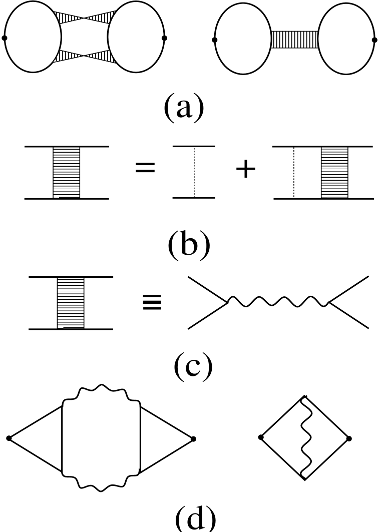
FIG. 4.: (a) The two one-loop diagrams for $R(\omega)$ in a disordered metal. The diagram on the left gives the (dominant) Altshuler-Shklovskii contribution; that on the right is smaller by a factor $\Delta\tau$, and is usually ignored. (b) Definition of the impurity ladders occuring in (a). (c) Rewriting the impurity ladder as an effective propagator. (d) Rewriting the diagrams in (a) using the notation of (c). The electron Green’s function lines end up in the so-called Hikami boxes.

Only the connected diagrams contribute to $R(\omega)$, while the trivial unconnected diagrams are cancelled by $-1$ in the definition of $R(\omega)$, Eq. (3).

Similarly, $p(\omega)$ is given by

$$p(\omega) = \frac{2\pi}{\rho L^{d}}\int\!\!d^{d}r\,\left<\rho(E+\omega,\mathchoice{{\hbox{\boldmath$\displaystyle r$}}}{{\hbox{\boldmath$\textstyle r$}}}{{\hbox{\boldmath$\scriptstyle r$}}}{{\hbox{\boldmath$\scriptscriptstyle r$}}})\rho(E,\mathchoice{{\hbox{\boldmath$\displaystyle r$}}}{{\hbox{\boldmath$\textstyle r$}}}{{\hbox{\boldmath$\scriptstyle r$}}}{{\hbox{\boldmath$\scriptscriptstyle r$}}})\right>=-\frac{\Delta}{2\pi}\int\!\!d^{d}r\,\left<{\cal G}(\omega;\mathchoice{{\hbox{\boldmath$\displaystyle r$}}}{{\hbox{\boldmath$\textstyle r$}}}{{\hbox{\boldmath$\scriptstyle r$}}}{{\hbox{\boldmath$\scriptscriptstyle r$}}},\mathchoice{{\hbox{\boldmath$\displaystyle r$}}}{{\hbox{\boldmath$\textstyle r$}}}{{\hbox{\boldmath$\scriptstyle r$}}}{{\hbox{\boldmath$\scriptscriptstyle r$}}}){\cal G}(0;\mathchoice{{\hbox{\boldmath$\displaystyle r$}}}{{\hbox{\boldmath$\textstyle r$}}}{{\hbox{\boldmath$\scriptstyle r$}}}{{\hbox{\boldmath$\scriptscriptstyle r$}}},\mathchoice{{\hbox{\boldmath$\displaystyle r$}}}{{\hbox{\boldmath$\textstyle r$}}}{{\hbox{\boldmath$\scriptstyle r$}}}{{\hbox{\boldmath$\scriptscriptstyle r$}}})\right>\,.$$ (70)

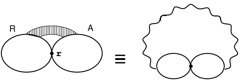
FIG. 5.: The one-loop diagram for the quantum return probability $p(\omega)$ in the ladder and Hikami-box representations.

The difference between the formulae (69) and (70) is that in the latter the densities of states are evaluated at the same point $\textstyle r$ in space rather than at different points. In diagrammatic terms this means that $p(\omega)$ consists of two loops connected to a single external point $\textstyle r$, as shown in Fig. (5).

In the diffusive regime of the disordered metal it is impurity ladders describing diffusive motion which give the important energy dependent contributions. They must have both a $R$ and $A$ line – so only $RA$ and $AR$ diagrams can contribute. Since the latter are complex conjugates of each other it follows that we can write the expressions for $R(\omega)$ and $p(\omega)$ in the following form:

$$R(\omega) = \frac{\Delta^{2}}{2\pi^{2}}\,\Re\text{e}\int\!\!d^{d}r\int\!\!d^{d}r\,^{\prime}\left<G^{R}(\omega;\mathchoice{{\hbox{\boldmath$\displaystyle r$}}}{{\hbox{\boldmath$\textstyle r$}}}{{\hbox{\boldmath$\scriptstyle r$}}}{{\hbox{\boldmath$\scriptscriptstyle r$}}},\mathchoice{{\hbox{\boldmath$\displaystyle r$}}}{{\hbox{\boldmath$\textstyle r$}}}{{\hbox{\boldmath$\scriptstyle r$}}}{{\hbox{\boldmath$\scriptscriptstyle r$}}})G^{A}(0;\mathchoice{{\hbox{\boldmath$\displaystyle r$}}}{{\hbox{\boldmath$\textstyle r$}}}{{\hbox{\boldmath$\scriptstyle r$}}}{{\hbox{\boldmath$\scriptscriptstyle r$}}}^{\prime},\mathchoice{{\hbox{\boldmath$\displaystyle r$}}}{{\hbox{\boldmath$\textstyle r$}}}{{\hbox{\boldmath$\scriptstyle r$}}}{{\hbox{\boldmath$\scriptscriptstyle r$}}}^{\prime})\right>\,,$$ (71)

$$p(\omega) = \frac{\Delta}{\pi}\,\Re\text{e}\int\!\!d^{d}r\,\left<G^{R}(\omega;\mathchoice{{\hbox{\boldmath$\displaystyle r$}}}{{\hbox{\boldmath$\textstyle r$}}}{{\hbox{\boldmath$\scriptstyle r$}}}{{\hbox{\boldmath$\scriptscriptstyle r$}}},\mathchoice{{\hbox{\boldmath$\displaystyle r$}}}{{\hbox{\boldmath$\textstyle r$}}}{{\hbox{\boldmath$\scriptstyle r$}}}{{\hbox{\boldmath$\scriptscriptstyle r$}}})G^{A}(0;\mathchoice{{\hbox{\boldmath$\displaystyle r$}}}{{\hbox{\boldmath$\textstyle r$}}}{{\hbox{\boldmath$\scriptstyle r$}}}{{\hbox{\boldmath$\scriptscriptstyle r$}}},\mathchoice{{\hbox{\boldmath$\displaystyle r$}}}{{\hbox{\boldmath$\textstyle r$}}}{{\hbox{\boldmath$\scriptstyle r$}}}{{\hbox{\boldmath$\scriptscriptstyle r$}}})\right>\,.$$ (72)

The impurity ladders (Fig. 4b) which connect the two loops describe either diffuson or Cooperon propagators given in momentum space by

$$D(q;\omega)=\frac{1}{2\pi\rho t_{el}^{2}}\,\frac{1}{Dq^{2}-i\omega}\,.$$ (73)

We will consider both the cases with and without time-reversal symmetry, referring to them as the orthogonal case ($\beta=1$) and unitary case ($\beta=2$). Diagrammatically, the latter differs from the former by the absence of the Cooperon contributions which are time-reversed impurity ladders.

The loops could be connected by arbitrary number of the ladders. In the lowest order there are the two contributions to $R(\omega)$ shown in Fig. 4a, and one contribution to $p(\omega)$ (Fig. 5). The dominant contribution to $R(\omega)$ – which is called Altshuler-Shklovskii diagram – has two impurity ladders; the diagram with only one ladder gives much smaller contribution.

Thus the perturbation order of a diagram is not determined by the number of ladders. A standard way [24, 25] to determine this order, and to make the calculation of diagrams more straightforward is rewriting them in the form where impurity ladders are represented as propagators (a wavy line in Fig. 4c); this is convenient since the ladders involve small momentum, $q\ell\ll 1$, and energy, $\omega t_{el}\ll 1$. All other Green’s function lines are absorbed into effective interactions between propagators (as shown in Figs. 4 and 5) known as Hikami boxes. Then the order of a diagram is the number of independent momenta occuring in the propagators, which is just the number of loops made of the wavy lines. (Each box corresponds to a single spatial point $\textstyle r$ and can be thought of as being contracted into a point; thus any diagram would consist of some number of wavy loops). The loop-expansion parameter here is $1/g$ where $g$ is the dimensionless conductance of the sample.

The one-loop diagrams for $R(\omega)$ are shown in Fig. 4d. The two external vertices may be in separate (odd) boxes, or the same (even) box; we ignore the latter since they are smaller than the former by factor $\Delta t_{el}\sim(\ell/L)^{d}$ in the same order of perturbation theory. The remaining Hikami boxes that do not contain an external vertex have an even number of sides.

Rewriting diagrams for $p(\omega)$ in terms of Hikami boxes we find that the external vertex (corresponding to the point $\textstyle r$ in Eq. (72)) has two boxes connected to it – these can either both be odd boxes, or both be “2-gons” (larger even boxes are not allowed since one can always string impurity ladders across them to recover the “2-gon” structure). All other boxes have no external vertex and so have an even number of sides. Note that all the Hikami boxes must be “dressed”, i.e. single-impurity lines should connect (without mutual intersection) those non-adjacent sides of the boxes which have the same analyticity (both $R$, or both $A$)[25]. In all diagrams below the boxes are assumed to be dressed. The one-loop contribution to $p(\omega)$ is given in Fig. 5 in both the ladder and Hikami representations. All the two-loop contributions to $p(\omega)$ and $R(\omega)$ are given in the Hikami representation in Fig. 6.

FIG. 6.: Two loop order diagrams to: $R(\omega)$ (a, b, c); $\widetilde{p}(\omega)$ (d, e); and $\widetilde{Q}(\omega)$ (f). All diagrams contribute in the orthogonal case, while only (d) and (f) contribute in the unitary case.

Before comparing the higher-order contributions made to Eq. (5) by the diagrams for $R(\omega)$ and $p(\omega)$, we consider the three-level correlator $Q(\omega^{\prime},\omega)$. Starting from Eq. (61), and rewriting the densities of states via Eq. (67) we get

$$Q(\omega^{\prime},\omega)=\Delta\left(\frac{i}{2\pi}\right)^{3}\int\!\!d^{d}r\,\int\!\!d^{d}r\,^{\prime}\Bigl{<}{\cal G}(0;\mathchoice{{\hbox{\boldmath$\displaystyle r$}}}{{\hbox{\boldmath$\textstyle r$}}}{{\hbox{\boldmath$\scriptstyle r$}}}{{\hbox{\boldmath$\scriptscriptstyle r$}}},\mathchoice{{\hbox{\boldmath$\displaystyle r$}}}{{\hbox{\boldmath$\textstyle r$}}}{{\hbox{\boldmath$\scriptstyle r$}}}{{\hbox{\boldmath$\scriptscriptstyle r$}}}){\cal G}(\omega^{\prime};\mathchoice{{\hbox{\boldmath$\displaystyle r$}}}{{\hbox{\boldmath$\textstyle r$}}}{{\hbox{\boldmath$\scriptstyle r$}}}{{\hbox{\boldmath$\scriptscriptstyle r$}}},\mathchoice{{\hbox{\boldmath$\displaystyle r$}}}{{\hbox{\boldmath$\textstyle r$}}}{{\hbox{\boldmath$\scriptstyle r$}}}{{\hbox{\boldmath$\scriptscriptstyle r$}}}){\cal G}(\omega;\mathchoice{{\hbox{\boldmath$\displaystyle r$}}}{{\hbox{\boldmath$\textstyle r$}}}{{\hbox{\boldmath$\scriptstyle r$}}}{{\hbox{\boldmath$\scriptscriptstyle r$}}}^{\prime},\mathchoice{{\hbox{\boldmath$\displaystyle r$}}}{{\hbox{\boldmath$\textstyle r$}}}{{\hbox{\boldmath$\scriptstyle r$}}}{{\hbox{\boldmath$\scriptscriptstyle r$}}}^{\prime})\Bigr{>}$$ (74)

Following the procedure used for $R(\omega)$ and $p(\omega)$ above we see that in the ladder representation the diagrams for $Q(\omega^{\prime},\omega)$ consist of three loops, two of which are joined at the external vertex $\textstyle r$, and the third having the external vertex $\mathchoice{{\hbox{\boldmath$\displaystyle r$}}}{{\hbox{\boldmath$\textstyle r$}}}{{\hbox{\boldmath$\scriptstyle r$}}}{{\hbox{\boldmath$\scriptscriptstyle r$}}}^{\prime}$. There are now several classes of diagrams that are not fully connected, as shown in Fig. (7a). (The shaded strips there include symbolically all possible combinations of impurity ladders). The most trivial has all loops unconnected and yields a constant term. The two others are reducible as they have only two out of the three loops connected by impurity ladders, and contribute terms proportional to $\rho^{3}R(\omega)$, $\rho^{3}R(\omega^{\prime}-\omega)$ and $\rho p(\omega^{\prime})$. These reducible contributions add up to give

$$Q_{uc}(\omega^{\prime},\omega)=\left(\frac{\rho L^{d}}{2\pi}\right)\left\{2\pi\rho[1+R(\omega)+R(\omega^{\prime}\!-\!\omega)]+p(\omega^{\prime})\right\}$$ (75)

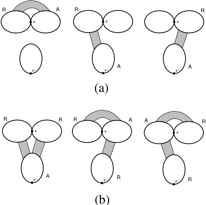
FIG. 7.: (a) The reducible contributions to the three-level correlator $Q(\omega^{\prime},\omega)$. The first diagram yields no contribution to the function $Q(t)$, whilst the other two yield equal contributions to $Q(t)$ that are proportional to $K(t)$. (b) The irreducible contributions to the three-level correlator $Q(\omega^{\prime},\omega)$. For analyticity reasons the last two diagrams give no contribution to the function $Q(t)$, so we need consider only diagrams of the first type.

We see that the r.h.s.  of the above is similar , but not identical to, the first line of the r.h.s.  of Eq. (65). The difference is that the is no $p(\omega^{\prime})$ multiplying the $R(\omega)$ and $R(\omega^{\prime}\!-\!\omega)$ in Eq. (75), only its constant part $2\pi\rho$. If we substitute this term into Eq. (50) we obtain $K(t)=(2\pi\hbar)^{-1}tp(t)$. In other words, the reducible diagrams of the three-level correlator $Q$ are enough to reproduce the diagonal approximation of semi-classics. In order to recover our formula, Eq. (5), we will need to analyze the irreducible contributions to $Q$ given schematically in Fig. 7b.

If we look at the irreducible contributions the first thing to note is that each diagram can only have ladders between two of the three pairs of loops. This is because ladders are always between an $R$ and an $A$ line, and so in an irreducible diagram either two loops are $R$ and the third $A$ or vice versa. There are therefore 6 possibilities which come in complex conjugate pairs: $AAR$ and $RRA$; $ARA$ and $RAR$; $RAA$ and $ARR$. The irreducible part of $Q(\omega^{\prime},\omega)$ can then be written in the form

$$\begin{array}[]{c}\displaystyle Q_{c}(\omega^{\prime},\omega)=\frac{1}{4\pi^{3}\rho L^{d}}\int\!\!d^{d}r\int\!\!d^{d}r\,^{\prime}\Im{\text{m}}\left\{\left<G^{A}(0;\mathchoice{{\hbox{\boldmath$\displaystyle r$}}}{{\hbox{\boldmath$\textstyle r$}}}{{\hbox{\boldmath$\scriptstyle r$}}}{{\hbox{\boldmath$\scriptscriptstyle r$}}},\mathchoice{{\hbox{\boldmath$\displaystyle r$}}}{{\hbox{\boldmath$\textstyle r$}}}{{\hbox{\boldmath$\scriptstyle r$}}}{{\hbox{\boldmath$\scriptscriptstyle r$}}})G^{A}(\omega;\mathchoice{{\hbox{\boldmath$\displaystyle r$}}}{{\hbox{\boldmath$\textstyle r$}}}{{\hbox{\boldmath$\scriptstyle r$}}}{{\hbox{\boldmath$\scriptscriptstyle r$}}},\mathchoice{{\hbox{\boldmath$\displaystyle r$}}}{{\hbox{\boldmath$\textstyle r$}}}{{\hbox{\boldmath$\scriptstyle r$}}}{{\hbox{\boldmath$\scriptscriptstyle r$}}})G^{R}(\omega^{\prime};\mathchoice{{\hbox{\boldmath$\displaystyle r$}}}{{\hbox{\boldmath$\textstyle r$}}}{{\hbox{\boldmath$\scriptstyle r$}}}{{\hbox{\boldmath$\scriptscriptstyle r$}}}^{\prime},\mathchoice{{\hbox{\boldmath$\displaystyle r$}}}{{\hbox{\boldmath$\textstyle r$}}}{{\hbox{\boldmath$\scriptstyle r$}}}{{\hbox{\boldmath$\scriptscriptstyle r$}}}^{\prime})\right>\right.\\ \displaystyle\left.+\left<G^{A}(0;\mathchoice{{\hbox{\boldmath$\displaystyle r$}}}{{\hbox{\boldmath$\textstyle r$}}}{{\hbox{\boldmath$\scriptstyle r$}}}{{\hbox{\boldmath$\scriptscriptstyle r$}}},\mathchoice{{\hbox{\boldmath$\displaystyle r$}}}{{\hbox{\boldmath$\textstyle r$}}}{{\hbox{\boldmath$\scriptstyle r$}}}{{\hbox{\boldmath$\scriptscriptstyle r$}}})G^{R}(\omega;\mathchoice{{\hbox{\boldmath$\displaystyle r$}}}{{\hbox{\boldmath$\textstyle r$}}}{{\hbox{\boldmath$\scriptstyle r$}}}{{\hbox{\boldmath$\scriptscriptstyle r$}}},\mathchoice{{\hbox{\boldmath$\displaystyle r$}}}{{\hbox{\boldmath$\textstyle r$}}}{{\hbox{\boldmath$\scriptstyle r$}}}{{\hbox{\boldmath$\scriptscriptstyle r$}}})G^{A}(\omega^{\prime};\mathchoice{{\hbox{\boldmath$\displaystyle r$}}}{{\hbox{\boldmath$\textstyle r$}}}{{\hbox{\boldmath$\scriptstyle r$}}}{{\hbox{\boldmath$\scriptscriptstyle r$}}}^{\prime},\mathchoice{{\hbox{\boldmath$\displaystyle r$}}}{{\hbox{\boldmath$\textstyle r$}}}{{\hbox{\boldmath$\scriptstyle r$}}}{{\hbox{\boldmath$\scriptscriptstyle r$}}}^{\prime})\right>+\left<G^{R}(0;\mathchoice{{\hbox{\boldmath$\displaystyle r$}}}{{\hbox{\boldmath$\textstyle r$}}}{{\hbox{\boldmath$\scriptstyle r$}}}{{\hbox{\boldmath$\scriptscriptstyle r$}}},\mathchoice{{\hbox{\boldmath$\displaystyle r$}}}{{\hbox{\boldmath$\textstyle r$}}}{{\hbox{\boldmath$\scriptstyle r$}}}{{\hbox{\boldmath$\scriptscriptstyle r$}}})G^{A}(\omega;\mathchoice{{\hbox{\boldmath$\displaystyle r$}}}{{\hbox{\boldmath$\textstyle r$}}}{{\hbox{\boldmath$\scriptstyle r$}}}{{\hbox{\boldmath$\scriptscriptstyle r$}}},\mathchoice{{\hbox{\boldmath$\displaystyle r$}}}{{\hbox{\boldmath$\textstyle r$}}}{{\hbox{\boldmath$\scriptstyle r$}}}{{\hbox{\boldmath$\scriptscriptstyle r$}}})G^{A}(\omega^{\prime};\mathchoice{{\hbox{\boldmath$\displaystyle r$}}}{{\hbox{\boldmath$\textstyle r$}}}{{\hbox{\boldmath$\scriptstyle r$}}}{{\hbox{\boldmath$\scriptscriptstyle r$}}}^{\prime},\mathchoice{{\hbox{\boldmath$\displaystyle r$}}}{{\hbox{\boldmath$\textstyle r$}}}{{\hbox{\boldmath$\scriptstyle r$}}}{{\hbox{\boldmath$\scriptscriptstyle r$}}}^{\prime})\right>\right\}\end{array}$$ (78)

When rewritten in the Hikami-box representation the diagrams for $Q$ consist of the two boxes connected to external vertex $\textstyle r$ found in $p(\omega)$ diagrams, plus a single odd box connected to external point $\mathchoice{{\hbox{\boldmath$\displaystyle r$}}}{{\hbox{\boldmath$\textstyle r$}}}{{\hbox{\boldmath$\scriptstyle r$}}}{{\hbox{\boldmath$\scriptscriptstyle r$}}}^{\prime}$ as found in $R(\omega)$ diagrams; these are then held together by wavy lines and even boxes with no external vertices. $Q_{AAR}$ diagrams cannot have the “2-gon” structure in the part connected to external point $\textstyle r$ since such a structure ends in ladders, which cannot happen here as both lines of the ladder would be $A$. $Q_{ARA}$ and $Q_{RAA}$ diagrams can have this “2-gon” structure.

If we are to re-derive our main result Eq. (5) diagrammatically we will need to show that the connected part of $Q(\omega^{\prime},\omega)$ factors into a product of $R$ and $p$. This can be seen by recalling the derivation of Eq. (5) via the Kirkwood approximation, where such factorization occurs in the first line of Eq. (65). The fact that only two pairs of loops can have ladders between them suggests a possible reason for this to occur. At this point we note that we are interested not in $Q(\omega^{\prime},\omega)$ itself but rather in $Q(t)$ which is derived from it by Fourier transforms as in Eq. (55). The analyticity properties of $Q(\omega^{\prime},\omega)$ diagrams will lead to some types giving no contribution to $Q(t)$. Eventually, a factorization emerges from this analysis which is different to that suggested in Eq. (65), but which, remarkably, yields the same spectral form factor in two dimensions, to third-loop order.

B Analytical properties of the three-level correlation function

First let us prove that only the $Q_{AAR}$ diagrams survive, starting with the formula for $Q(t)$ given by Eq. (3),

$$\begin{array}[]{rcl}Q(t)&=&\displaystyle\int_{0}^{t}dt^{\prime}\int d\omega^{\prime}\int d\omega e^{-i\omega^{\prime}t^{\prime}}e^{i\omega t}Q(\omega^{\prime},\omega)\\ &=&\displaystyle\int d\omega^{\prime}\int d\omega{e^{i\omega t}-e^{i(\omega-\omega^{\prime})t}\over i\omega^{\prime}}Q(\omega^{\prime},\omega)\end{array}$$ (81)

Taking the Fourier transform of $Q(t)$ then yields

$$\begin{array}[]{rl}&\displaystyle\int dte^{i\overline{\omega}t}\int d\omega^{\prime}\int d\omega\frac{e^{i\omega t}-e^{i(\omega-\omega^{\prime})t}}{i\omega^{\prime}}Q(\omega^{\prime},\omega)\\ =2\pi&\displaystyle\int d\omega^{\prime}\int d\omega\frac{1}{i\omega^{\prime}}\left[\delta(\overline{\omega}+\omega)-\delta(\overline{\omega}+\omega-\omega^{\prime})\right]Q(\omega^{\prime},\omega)\\ =-2\pi i&\displaystyle\int\frac{d\omega^{\prime}}{\omega^{\prime}}\left[Q(\omega^{\prime},-\overline{\omega})-Q(\omega^{\prime},\omega^{\prime}-\overline{\omega})\right]\end{array}$$ (85)

Now consider the analyticity properties of the $ARR$, $ARA$ and $AAR$ respectively. They can be written in the form

$$Q_{RAA}(\omega^{\prime},\omega) = f(-\omega^{\prime},-\omega)$$ (86)

$$Q_{ARA}(\omega^{\prime},\omega) = f(\omega^{\prime},\omega^{\prime}-\omega)$$ (87)

$$Q_{AAR}(\omega^{\prime},\omega) = f(\omega,\omega-\omega^{\prime})\,.$$ (88)

where in each case $f(\omega_{1},\omega_{2})$ is a function analytic in the u.h.p. for both arguments. For $Q_{RAA}$ Eq. (85) gives

$$-2\pi i\int{d\omega^{\prime}\over\omega^{\prime}}\left[f(-\omega^{\prime},\overline{\omega})-f(-\omega^{\prime},-\omega^{\prime}+\overline{\omega})\right]=-2\pi^{2}\left[f(0,-\overline{\omega})-f(0,-\overline{\omega})\right]=0\,,$$ (89)

since upon closing each term in l.h.p. we only get contributions from the pole at $\omega^{\prime}=0$, and these cancel. Similarly for $Q_{ARA}$ we get upon closing in the u.h.p.

$$-2\pi i\int{d\omega^{\prime}\over\omega^{\prime}}\left[f(\omega^{\prime},\omega^{\prime}+\overline{\omega})-f(\omega^{\prime},\overline{\omega})\right]=2\pi^{2}\left[f(0,\overline{\omega})-f(0,\overline{\omega})\right]=0\,.$$ (90)

Finally for $Q_{AAR}$ we get

$$-2\pi i\int{d\omega^{\prime}\over\omega^{\prime}}\left[f(-\overline{\omega},-\omega^{\prime}-\overline{\omega})-f(\omega^{\prime}-\overline{\omega},-\overline{\omega})\right]=-(2\pi)^{2}f(-\overline{\omega},-\overline{\omega})\,.$$ (91)

where we closed first term in l.h.p., second in u.h.p. to yield contributions that add up. The above term can be rewritten in the form $-(2\pi)^{2}Q_{AAR}(\omega^{\prime}=0,-\overline{\omega})$, so it follows that diagrams for $Q_{AAR}$ can yield Fourier transform of $Q(t)$ directly. We have therefore verified our previous assertion, and moreover have derived the contribution to the Fourier transform of $Q(t)$ coming from the $Q_{AAR}$ diagrams. Diagrammatically the above means that all ladders in $Q_{AAR}$ diagrams will have the same energy dependence.

Let us discuss what the above means for our factorization hypothesis. The reason we expected that it would be the $Q_{RAR}$ and $Q_{ARR}$ diagrams that survived is that we can envisage a natural factorization into terms with energy dependence of the form $R(\omega)p(\omega^{\prime})$ and $R(\omega^{\prime}-\omega)p(\omega^{\prime})$, which are exactly what is needed to reproduce Eq. (5). The fact that it is $Q_{AAR}$ which survives means that our factorization hypothesis must be altered to have an energy dependence $R(\omega)p(\omega)$, which leads to a convolution in $t$-space. More precisely, we expect the $\omega$-space factorization to have the form

$$\widetilde{Q}(\omega)=-\frac{(2\pi)^{2}i}{\Delta}\,\widetilde{p}(\omega)\,\widetilde{R}(\omega)\,.$$ (92)

Here we have introduced the analytical functions $\widetilde{Q}(\omega),\,\widetilde{p}(\omega)$ and $\widetilde{R}(\omega)$ as follows:

$$\begin{array}[]{rcl}\widetilde{Q}(\omega)&\equiv&Q_{AAR}(0,\,\omega)\,;\\ {p}(\omega)&\equiv&2\Re\text{e}\,\widetilde{p}(\omega)\,;\\ {R}(\omega)&\equiv&2\Re\text{e}\,\widetilde{R}(\omega)\,.\end{array}$$ (96)

Note that diagrammatically we calculate exactly these analytical functions. Before giving the results for higher-loop contributions, note that calculations of $\widetilde{R}(\omega)$ are considerably simplified due to the fact that it can be obtained as the second derivative of “free energy” $F(\omega)$:

$$\widetilde{R}(\omega)=-\left({\Delta\over 2\pi}\right)^{2}\frac{\partial^{2}}{\partial\omega^{2}}\widetilde{F}(\omega)$$ (97)

Here $F(\omega)$ is given by the sum of all diagrams that have no external vertices, and the coefficient of proportionality is chosen so as to make $F(\omega)$ dimensionless.

C Calculation of diagrams up to three-loop order

As a result of the above discussion we can now lay out the diagrammatic program ahead. First, we will calculate the contributions to $\widetilde{F}(\omega)$, $\widetilde{p}(\omega)$, and $\widetilde{Q}(\omega)$ up to three-loop order. Then we will first verify Eq. (50) (which has been obtained assuming spectral homogeneity), and then check the factorization scheme of Eq. (92) which is dictated by the analytical structure described above. This factorization is equivalent to that given by Eq. (9). Finally, we will show how, having verified this factorization up to the three-loop order, to check the factorization that comes out of the Kirkwood approximation, Eq. (65), and is equivalent to the result of the Brownian-motion model, Eq. (5). We will show that up to the third-loop order both the factorizations are identical and exact. Therefore, Eq. (5) obtained within the Brownian motion picture turn out to be correct to quite a nontrivial order of perturbation theory.

Let us introduce a notation that is convenient for further analysis:

$${\cal P}_{1\ldots n}\equiv D(\mathchoice{{\hbox{\boldmath$\displaystyle q$}}}{{\hbox{\boldmath$\textstyle q$}}}{{\hbox{\boldmath$\scriptstyle q$}}}{{\hbox{\boldmath$\scriptscriptstyle q$}}}_{1}+\ldots+\mathchoice{{\hbox{\boldmath$\displaystyle q$}}}{{\hbox{\boldmath$\textstyle q$}}}{{\hbox{\boldmath$\scriptstyle q$}}}{{\hbox{\boldmath$\scriptscriptstyle q$}}}_{n})^{2}-i\omega$$ (98)

In particular, ${\cal P}_{1}\equiv Dq_{1}^{2}-i\omega$.

Now, two-loop order contributions corresponding to the diagrams in Fig. 8(a) (equivalent to those in Fig. 6a–c) and in Fig. 6(d–f) may be written as

$$\widetilde{F}_{2}(\omega) = \left({2-\beta\over\beta}\right){\Delta\over 2\pi}\sum_{q_{1},q_{2}}\frac{{\cal P}_{1}+{\cal P}_{2}+i\omega}{{\cal P}_{1}\,{\cal P}_{2}}\,;$$ (99)

$$\widetilde{p}_{2}(\omega) = \left({2\over\beta}\right){\Delta\over 2\pi L^{d}}\Re\text{e}\sum_{q_{1},q_{2}}\left\{\frac{1}{{\cal P}_{1}\,{\cal P}_{2}}+2(2-\beta)\frac{{\cal P}_{1}+{\cal P}_{2}+i\omega}{\bigl{(}{\cal P}_{1}\bigr{)}^{2}\,{\cal P}_{2}}\right\}\,;$$ (100)

$$\widetilde{Q}_{2}(\omega) = -i\left({2\over\beta}\right)^{2}{\Delta\over L^{d}}\sum_{q_{1},q_{2}}\frac{1}{\bigl{(}{\cal P}_{1}\bigr{)}^{2}\,{\cal P}_{2}}$$ (101)

Here we note the following. The diagrammatic approach could be used both in the diffusive regime, $\omega\gg E_{c}$, where all the sums above should be replaced by integrals, and in the ergodic regime, $E_{c}\gg\omega\gg\Delta$, where only contribution of zero mode (all $\mathchoice{{\hbox{\boldmath$\displaystyle q$}}}{{\hbox{\boldmath$\textstyle q$}}}{{\hbox{\boldmath$\scriptstyle q$}}}{{\hbox{\boldmath$\scriptscriptstyle q$}}}=0$) survives. In the diffusive regime, regularization of divergent integrals is required. Although we do not explicitly calculate contributions of all diagrams below, in all algebraic manipulations we use dimensional regularization near $d=2$. These manipulations involve dealing with large $q\sim\ell^{-1}$, and so all diagrammatic expressions we give here are not directly valid in the ergodic regime. However, it is straightforward to verify the accuracy of our factorization scheme in the zero-mode regime as well.

The three-loop contributions to $F(\omega)$, $p(\omega)$, and $Q(\omega)$ are shown in Figs. 8, 9, and 10, respectively. In Fig. 8a we have also drawn the two-loop contribution to $F(\omega)$ which is equivalent to the three two-loop contributions to $R(\omega)$ shown in Fig. 6. Note that in the three-loop order there are 41 diagrams that contribute directly to $R(\omega)$, so that to have instead only the 5 diagrams for $F(\omega)$, as in Fig. 8, is a considerable simplification. Nevertheless, these three-loop results are quite bulky, and we list contributions of

FIG. 8.: Two and three-loop order diagrams for the function $\widetilde{F}(\omega)$. The two-loop diagram is equivalent to those in Fig. 6(a–c), and contributes only to the orthogonal case. All 5 three-loop diagrams contribute to the orthogonal case, while only 3a and 3b contribute to the unitary case.

FIG. 9.: Three-loop order diagrams for the quantum return probability $\widetilde{p}(\omega)$. All 10 diagrams contribute in the orthogonal case, while only the first 2 contribute in the unitary case.

FIG. 10.: Three loop order diagrams for the function $\widetilde{Q}(\omega)$. All 13 diagrams contribute in the orthogonal case, whilst only the first 4 contribute in the unitary case.

each diagram in the three tables.

$\displaystyle 3F_{a}$ $\displaystyle=$ $\displaystyle F_{d}=-2\sum_{q_{1},q_{2},q_{3}}\frac{2({\cal P}_{1}+{\cal P}_{2}+{\cal P}_{3})+3i\omega}{{\cal P}_{1}{\cal P}_{2}{\cal P}_{3}}$ $\displaystyle F_{b}$ $\displaystyle=$ $\displaystyle\frac{1}{4}\sum_{q_{1},q_{2},q_{3}}\frac{({\cal P}_{12}+{\cal P}_{23})^{2}}{{\cal P}_{1}{\cal P}_{2}{\cal P}_{3}{\cal P}_{123}}$ $\displaystyle F_{c}$ $\displaystyle=$ $\displaystyle 2\sum_{q_{1},q_{2},q_{3}}\frac{({\cal P}_{1}+{\cal P}_{2}+i\omega)({\cal P}_{1}+{\cal P}_{3}+i\omega)}{{\cal P}_{1}^{2}{\cal P}_{2}{\cal P}_{3}}$ $\displaystyle F_{e}$ $\displaystyle=$ $\displaystyle\frac{1}{2}\sum_{q_{1},q_{2},q_{3}}\frac{({\cal P}_{12}+{\cal P}_{23})({\cal P}_{13}+{\cal P}_{32})}{{\cal P}_{1}{\cal P}_{2}{\cal P}_{3}{\cal P}_{123}}$         Table 1. Three-loop order contributions to $\widetilde{F}(\omega)$: an overall factor of $(\Delta/2\pi)^{2}$ should be attached to each contribution.

$\displaystyle p_{a}$ $\displaystyle=$ $\displaystyle\frac{1}{2}p_{e}=p_{f}=-2\sum_{q_{1},q_{2},q_{3}}\frac{2({\cal P}_{1}+{\cal P}_{2}+{\cal P}_{3})+3i\omega)}{{\cal P}_{1}^{2}{\cal P}_{2}{\cal P}_{3}}$ $\displaystyle p_{b}$ $\displaystyle=$ $\displaystyle\sum_{q_{1},q_{2},q_{3}}\frac{({\cal P}_{12}+{\cal P}_{23})^{2}}{{\cal P}_{1}^{2}{\cal P}_{2}{\cal P}_{3}{\cal P}_{123}}$ $\displaystyle p_{c}$ $\displaystyle=$ $\displaystyle 4\sum_{q_{1},q_{2},q_{3}}\frac{({\cal P}_{1}+{\cal P}_{2}+i\omega)({\cal P}_{1}+{\cal P}_{3}+i\omega)}{{\cal P}_{1}^{3}{\cal P}_{2}{\cal P}_{3}}$ $\displaystyle p_{d}$ $\displaystyle=$ $\displaystyle 4\sum_{q_{1},q_{2},q_{3}}\frac{({\cal P}_{1}+{\cal P}_{2}+i\omega)({\cal P}_{2}+{\cal P}_{3}+i\omega)}{{\cal P}_{1}^{2}{\cal P}_{2}^{2}{\cal P}_{3}}$ $\displaystyle p_{g}$ $\displaystyle=$ $\displaystyle 2\sum_{q_{1},q_{2},q_{3}}\frac{({\cal P}_{12}+{\cal P}_{23})({\cal P}_{13}+{\cal P}_{32})}{{\cal P}_{1}^{2}{\cal P}_{2}{\cal P}_{3}{\cal P}_{123}}$ $\displaystyle p_{h}$ $\displaystyle=$ $\displaystyle 4\sum_{q_{1},q_{2},q_{3}}\frac{({\cal P}_{1}+{\cal P}_{2}+i\omega)}{{\cal P}_{1}^{2}{\cal P}_{2}{\cal P}_{3}}$ $\displaystyle p_{i}$ $\displaystyle=$ $\displaystyle-4\sum_{q_{1},q_{2},q_{3}}\frac{1}{{\cal P}_{1}{\cal P}_{2}{\cal P}_{3}}$ $\displaystyle p_{j}$ $\displaystyle=$ $\displaystyle\sum_{q_{1},q_{2},q_{3}}\frac{({\cal P}_{12}+{\cal P}_{23})}{{\cal P}_{1}{\cal P}_{2}{\cal P}_{3}{\cal P}_{123}}$         Table 2. Three-loop order contributions to $\widetilde{p}(\omega)$: an overall factor of $L^{-d}(\Delta/2\pi)^{2}$ should be attached to each contribution.

$\displaystyle Q_{a}$ $\displaystyle=$ $\displaystyle 2Q_{b}=Q_{h}=Q_{i}=Q_{j}=Q_{k}=2i\sum_{q_{1},q_{2},q_{3}}\frac{1}{{\cal P}_{1}^{2}{\cal P}_{2}{\cal P}_{3}}$ $\displaystyle Q_{c}$ $\displaystyle=$ $\displaystyle Q_{l}=i\sum_{q_{1},q_{2},q_{3}}\frac{1}{{\cal P}_{1}{\cal P}_{2}{\cal P}_{3}{\cal P}_{123}}$ $\displaystyle Q_{d}$ $\displaystyle=$ $\displaystyle Q_{m}=-2i\sum_{q_{1},q_{2},q_{3}}\frac{({\cal P}_{12}+{\cal P}_{23})}{{\cal P}_{1}^{2}{\cal P}_{2}{\cal P}_{3}{\cal P}_{123}}$ $\displaystyle Q_{e}$ $\displaystyle=$ $\displaystyle-4i\sum_{q_{1},q_{2},q_{3}}\frac{({\cal P}_{1}+{\cal P}_{2}+i\omega)}{{\cal P}_{1}^{3}{\cal P}_{2}{\cal P}_{3}}$ $\displaystyle Q_{f}$ $\displaystyle=$ $\displaystyle-2i\sum_{q_{1},q_{2},q_{3}}\frac{({\cal P}_{1}+{\cal P}_{3}+i\omega)}{{\cal P}_{1}^{2}{\cal P}_{2}^{2}{\cal P}_{3}}$ $\displaystyle Q_{g}$ $\displaystyle=$ $\displaystyle-2i\sum_{q_{1},q_{2},q_{3}}\frac{({\cal P}_{1}+{\cal P}_{2}+i\omega)}{{\cal P}_{1}^{2}{\cal P}_{2}^{2}{\cal P}_{3}}$         Table 3. Three-loop order contributions to $\widetilde{Q}(\omega)$: an overall factor of $(\Delta^{2}/2\pi L^{d})$ should be attached to each contribution.

The labels in the tables correspond to those in Figs. 8–10, and in the figure captions we describe which diagrams are made of diffusons only and thus contribute in the unitary ($\beta=1$) case. Obviously, all the diagrams contribute in the orthogonal ($\beta=2$) case. Results for the symplectic symmetry class ($\beta=4$) are practically the same as for the orthogonal case but we do not list them here to avoid complications with the coefficients.

The starting point for our diagrammatic analysis is Eq. (50) which we now rewrite as follows. The Fourier transform, Eq. (3), of the function $Q(t)$ is split into the reducible and irreducible parts (Eqs. (75) and (78), respectively). As only $\widetilde{Q}(\omega)$, Eq. (96), contributes to the irreducible part, we obtain

$$\frac{\partial}{\partial(i\omega)}\left[\frac{1}{L^{d}}\frac{\partial}{\partial(i\omega)}F(\omega)-\widetilde{p}(\omega)\right]=\frac{i}{\pi}\widetilde{Q}(\omega)$$ (102)

This is the exact relation which holds to all orders in perturbation theory. It allows us to check the accuracy of our diagrammatics up to three loop order for both the unitary and orthogonal cases. We do this by first substituting the two-loop results of Eq. (99) - which is quite straightforward, and then the three-loop data from the tables which requires some significant algebra. We verify that this identity holds with our diagrammatic results which gives us confidence in their accuracy.

The next step is to see whether our projected $\omega$-space factorization occurs to two and three loop order in both the orthogonal and unitary cases. To check Eq. (92) up to two-loop order, we calculate both factors in the r.h.s. to the first order only. This is simple and yields

$$\widetilde{Q}_{2}(\omega)=-i\left(\frac{2}{\beta}\right)^{2}\sum_{q_{1},q_{2}}\frac{1}{\bigl{(}{\cal P}_{1}\bigr{)}^{2}\,{\cal P}_{2}}=-\frac{i(2\pi)^{2}}{\Delta}\,\widetilde{p}_{1}(\omega)\widetilde{R}_{1}(\omega)\,,$$

so that the factorization (92) is exact in this order. The reason why this is so simple is that with only two momenta $q_{1}$ and $q_{2}$ there is no way for the momenta to become “entangled”, and so there is only really one possible functional form. The fact that the numerical coefficients match up exactly is the important thing. The three loop case is more involved because now the entanglement can occur, and this leads to the factorization not being exact. For both the unitary and orthogonal case, however, we get the same functional form in the remainder,

$$Q_{3}(\omega)+\frac{i(2\pi)^{2}}{\Delta}\left[\widetilde{R}_{1}(\omega)\widetilde{p}_{2}(\omega)+\widetilde{R}_{2}(\omega)\widetilde{p}_{1}(\omega)\right]$$

$$= -\frac{2i\Delta^{2}}{\pi\beta^{2}L^{d}}\sum_{q_{1},q_{2},q_{3}}\left\{\frac{4}{\bigl{(}{\cal P}_{1}\bigr{)}^{2}\,{\cal P}_{2}\,{\cal P}_{3}}-\frac{2\bigl{(}{\cal P}_{12}+{\cal P}_{23}\bigr{)}}{\bigl{(}{\cal P}_{1}\bigr{)}^{2}\,{\cal P}_{2}\,{\cal P}_{3}\,{\cal P}_{123}}+\frac{1}{{\cal P}_{1}\,{\cal P}_{2}\,{\cal P}_{3}\,{\cal P}_{123}}\right\}\,.$$

The remainder can then be algebraically manipulated to give

$$\frac{2\Delta^{2}}{3\pi\beta^{2}L^{d}}\,\frac{\partial}{\partial(i\omega)}\sum_{q_{1},q_{2},q_{3}}\left\{\frac{i\omega}{{\cal P}_{1}\,{\cal P}_{2}\,{\cal P}_{3}\,{\cal P}_{123}}\right\}\,.$$ (103)

At the three loop level we see that the factorization is not exact, but that the remainder term is simple and its momentum integrals are fully convergent. Certainly for the orthogonal case many terms have been removed to yield this remainder. We next note that in the special case of two dimensions this remainder is zero, and the factorization is exact. This is because for $d=2$ dimensional analysis shows that the term inside the derivative is a constant – it is of the form $(-i\omega)^{0}$, and no logarithmic singularities are present – and so one gets zero upon taking derivative. Even if the remainder were not able to be written as a derivative, but just as a sum of terms with no logarithmic singularities, it would yield zero. This is because dimensional analysis shows that the result is of the form $a/(-i\omega)$, where $a$ is a real constant. Since we have to take the real part of this to get $R(\omega)$ this would give zero. However in this case there would be a constant contribution to the Fourier transform $K(t)$, because $a/(-i\omega)$ does actually have a real part proportional to $\delta(\omega)$ – this is exactly what happens in the case of the 1-loop contribution in $d=2$. We note that our factorization is exact to 3-loop order in $d=2$ even in the sense of getting the constant term in $K(t)$ correct.

It seems to us that the exactness of factorization up to three loop order in $d=2$ for both orthogonal and unitary cases is no accident, and we conjecture that this result persists to all orders in perturbation theory. Obviously such a conjecture cannot be proved using order-by-order analysis (although, of course, it could be disproved this way), so any attempt to verify this will require analysis of the structure of $R(\omega)$, $p(\omega)$, and $Q(\omega)$ diagrams.

D Comparison of the Two Factorization Schemes

In this section we will compare the two factorization schemes that we have introduced in this paper: the $t$-space scheme that arose from consideration of the Brownian motion model of section (III), and the $\omega$-space scheme that arose in the diagrammatic analysis of section (VI). We have shown that the $\omega$-space scheme is exact to 2-loop order in all dimensions, and to 3-loop order in the 2d case. We will now examine the validity of the $t$-space scheme. This involves very little extra work because most of the algebraic manipulation has already been performed in the $\omega$-space analysis. We first compare the two relations by writing both of them in $t$-space to yield

$$K(t)-(2\pi\hbar\rho)^{-1}tp(t) = -(\pi\hbar\rho)^{-1}\int_{0+}^{t}dt^{\prime}K(t^{\prime})p(t-t^{\prime})$$ (105)

$$K(t)-(2\pi\hbar\rho)^{-1}tp(t) = -(\pi\hbar\rho)^{-1}K(t)\int_{0}^{t}p(t^{\prime})$$ (106)

where, of course, we know the region of validity of the first formula. To investigate the $t$-space factorization we need only compare the r.h.s. of the above equations. In the 2-loop case the $K(t)$ and $p(t)$ in the r.h.s. will both be of 1-loop order, and we know that $p_{1}(t)\propto t^{-d/2}$ and $K_{1}(t)\propto t^{1-d/2}$. We find that the two equations above only agree for $d=2$, where $K_{1}(t)=1$. The $t$-space factorization is therefore exact to 2-loops only in 2d, and we restrict ourselves to the 2d case from now on.

To look at the $t$-space scheme to 3-loop order in 2d we note that we can have the combinations $K_{1}$, $p_{2}$, and $K_{2}$, $p_{1}$. For the unitary case $K_{2}(t)=0$, so this leaves only the first contribution, and since $K_{1}(t)=1$ the two factorizations become the same. For the orthogonal case we have to look at the second contribution. We find that the two equations differ by a constant. For the purpose of calculating the asymptotic behaviour of $R(\omega)$, constant terms in $K(t)$ have no effect, so that the $t$-space factorization works up to 3-loop order in 2d for both orthogonal and unitary cases.

At this point it seems that the $\omega$-space scheme may be perturbatively slightly more accurate than the $t$-space scheme in that it is correct in 2-loops for all dimensions, and at 3-loop order it gets the constant term in $K(t)$ correct in the orthogonal case. However we are still justified in saying that both schemes are correct to 3-loop order in 2d.

VII Summary

In this paper we have examined spectral correlations in disordered conductors, starting from the idea (Eq. 43) that two samples with impurity configurations differing by an infinitesimal amount should be statistically equivalent. In the first instance, this equivalence yields an identity relating two-point to three-point correlation functions; it is useful only if one can decouple the latter. We argue that a decoupling based on the Kirkwood superposition approximation is physically reasonable provided one is interested only in correlations at scales large compared to the mean level spacing. Within the approximation, we express (Eq. 5) both the non-parametric and the parametric spectral form factor in terms of the quantum return probability for a spreading wavepacket. We test the decoupling by calculating corrections, using the standard diagrammatic perturbation theory for disordered conductors to expand about the metallic limit in inverse powers of the dimensionless conductance, $g$. We show that in two-dimensional systems, the case of greatest interest, there are no corrections to order $g^{-3}$. We believe that the results we obtain from this approach should be useful rather generally, and especially when a diagrammatic analysis is not straightforward, as at the Anderson transition; the implications of our work in that regime will be discussed elsewhere.

- [1] E. P. Wigner, Proc. Cambridge Philos. Soc. 47, 790 (1951).
- [2] F. J. Dyson, J. Math. Phys. 3, 140 (1962).
- [3] M. L. Mehta, Random matrices (Academic Press, Boston, 1991).
- [4] L. P. Gor’kov and G. M. Eliashberg, Zh. Eksp. Teor. Fiz. 48, 1407 (1965) [Sov. Phys. JETP 21, 940 (1965)].
- [5] K. B. Efetov, Adv.Phys. 32, 53 (1983).
- [6] B. L. Altshuler and B. I. Shklovskii, Zh. Eksp. Teor. Fiz. 91, 220 (1986) [Sov. Phys. JETP 64, 127 (1986)].
- [7] N. Argaman, Y. Imry, and U. Smilansky, Phys. Rev. B 47, 4440 (1993).
- [8] J. T. Chalker, I. V. Lerner, and R. A. Smith, submitted to Phys. Rev. Lett., 1996.
- [9] F. J. Dyson, J. Math. Phys. 3, 1191 (1962).
- [10] P. Pechukas, Phys. Rev. Lett. 51, 943 (1983).
- [11] M. Wilkinson, J. Phys. A 21, 4021 (1990), P. Gaspard et al, Phys. Rev. A 42, 4015 (1990), J. Goldberg et al, Nonlinearity 4, 1 (1991).
- [12] A. Szafer and B. L. Altshuler, Phys. Rev. Lett. 70, 587 (1993).
- [13] B. D. Simons and B. L. Altshuler, Phys. Rev. Lett. 70, 4063 (1993).
- [14] B. D. Simons and B. L. Altshuler, Phys. Rev. B 48, 5422 (1993).
- [15] T. Yukawa, Phys. Rev. Lett. 54, 1883 (1985).
- [16] C. W. J. Beenakker, Phys. Rev. Lett. 70, 4126 (1993).
- [17] A. I. Larkin and D. E. Khmelnitskii, Uspekhi Fizicheskikh Nauk 136, 536 (1982).
- [18] D. E. Khmelnitskii, Physica B&C 126, 235 (1984).
- [19] V. E. Kravtsov and I. V. Lerner, Phys. Rev. Lett. 74, 2563 (1995).
- [20] In the ergodic regime, this expression gives only the envelope of the TLCF as the oscillations in [3] are due to singularities in near , which cannot be accounted for semi-classically.
- [21] F. J. Dyson, J. Math. Phys. 13, 90 (1972).
- [22] L. A. Pastur, Th. Math. Phys. 10, 67 (1972).
- [23] J. G. Kirkwood, J. Chem. Phys. 3, 300 (1935).
- [24] L. P. Gor’kov, A. I. Larkin, and D. E. Khmel’nitskii, Pis’ma v ZhETF 30, 248 (1979) [JETP Letters 30, 228 (1979)].
- [25] S. Hikami, Phys. Rev. B 24, 2671 (1981).