Integer Quantum Hall Effect in Double-Layer Systems

Abstract

We consider the localization of independent electron orbitals in double-layer two-dimensional electron systems in the strong magnetic field limit. Our study is based on numerical Thouless number calculations for realistic microscopic models and on transfer matrix calculations for phenomenological network models. The microscopic calculations indicate a crossover regime for weak interlayer tunneling in which the correlation length exponent appears to increase. Comparison of network model calculations with microscopic calculations casts doubt on their generic applicability.

]

I Introduction

The integer quantum Hall effect is generally well understood in single-layer two-dimensional electron systems (2DES’s) which are sufficiently disordered that interactions do not play an essential role and are in a field sufficiently strong that Landau level mixing does not play an essential role. In this limit, single-electron orbitals are localized except at a critical energy $E_{c}$ near the center of each disorder broadened Landau level. For Fermi energy $E_{F}=E_{c}$, theory [1, 2, 3, 4] predicts that $(\sigma_{xx}^{c},\sigma_{xy}^{c})=(1,2n+1)e^{2}/2h$ whereas on the Hall plateaus ($E_{F}\neq E_{c}$) $(\sigma_{xx},\sigma_{xy})=(0,n)e^{2}/h$ where $n$ is the number of extended state energies below the Fermi level. As the critical energy is approached, the localization length for electrons at the Fermi level is expected to have a power-law divergence, $\xi\sim|E_{F}-E_{c}|^{-\nu}$, and $\nu$, the correlation length exponent, is expected to be independent of $n$. It is believed that the transition is well described by quantum percolation [5, 6] models and semiclassical calculations [7] have estimated the correlation length exponent to $\nu=7/3$. This picture has been corroborated by a large number of thorough numerical studies [8, 9, 10, 11, 12] which are in agreement with theoretical predictions for $\sigma_{xx}^{c}$ and $\sigma_{xy}^{c}$. Localization properties and the divergence of the localization length have been studied extensively  [13, 14, 15, 16, 17, 18, 19, 20] with the most recent estimate of the correlation length exponent being $\nu=2.35\pm 0.03$ [20]. On the experimental side, measurements of the width, $\Delta B$, of the peak of $\rho_{xx}$ as well as $(d\rho_{xy}/dB)^{-1}$, both predicted to scale with temperature as $T^{1/z\nu}$, yield values $1/\nu=0.42\pm 0.04$[21, 22] with $z$ assumed to be 1. Higher derivatives of $\rho_{xy}$ yields exponents [23] of $n\nu$ in agreement with scaling theories of the transition between Hall plateaus. (Experiments in the fractional quantum Hall regime find similar values [24] for this exponent.) Recently the dynamical critical exponent, $z$, has been measured [25, 26] to be $z=1$.

In this paper we report on a numerical study of the localization properties of single-electron orbitals in double-layer two-dimensional electron systems. This work is motivated by recent experiments hinting at changes in localization properties when two different Landau levels are nearly degenerate [22, 23, 24, 25, 27, 28, 29], by growing interest in the conditions necessary for the occurrence of the quantum Hall effect in three-dimensional electron systems, and by the need for improved understanding of the disappearance of the quantum Hall effect at weak magnetic fields in high mobility samples. In each case, we believe that double-layer quantum Hall systems offer advantages for both theoretical studies and for the experimental studies which we hope to motivate.

In single-layer two-dimensional electron systems, localization properties appear experimentally to be changed when the exchange enhanced spin-splitting between Landau levels with the same orbital index collapses.[30] The interpretation of these experiments is confused by uncertainties involved in modeling the spin-orbit disorder scattering necessary for mixing the two Landau levels and by the the apparent importance of interaction effects in controlling the degree of mixing. The interaction complications are not so troublesome in double-layer systems and, in addition, the degree of mixing between Landau levels in separate quantum wells can be controlled by adjusting the strength of the barrier separating the wells or by adding an external bias potential which moves the double-layer system off balance.

In high-mobility two-dimensional electron systems ($E_{F}\tau/\hbar>>1$), the quantum Hall effect appears to become unobservable in practice once Landau level mixing by disorder becomes strong, i.e. once $\omega_{c}\tau$ is of order one. (Here $\omega_{c}=eB/m^{*}c$ is the cyclotron frequency.) The loss of an observable quantum Hall effect in these systems appears to be associated with a dramatic increase in the localization length in the middle of the Hall plateaus, rather than with the ‘floatation’ of extended state energies  [31, 32, 33, 34, 35, 36, 37] which occurs in more strongly disordered systems. It seems likely that the same dramatic increase in localization lengths on Hall plateaus will occur in double-layer systems when the Landau levels in the two-layers are strongly mixed. The ability to systematically control the number of Landau levels which are mixed motivates working with double and multi-layer systems.

Since much of the physical picture underlying the quantum Hall effect is specific to two dimensions, it was not initially clear that it was even possible to observe quantized plateaus in three-dimensional systems. Early experimental work, focused on widely separated 2D layers [38], found the IQHE with quantized resistivity $\rho_{xy}=h/N_{z}ie^{2}$ where $N_{z}$ is the number of quantum wells, consistent with parallel conduction in many quantum wells. Störmer et al. [39] performed experiments on coupled GaAs superlattices with 30 periods, where the dispersion relations explicitly showed three-dimensional effects in zero magnetic field. Measurements of the resistivity tensor showed that $\rho_{xy}$ again was quantized as $h/nie^{2}$ despite the 3D nature of the system, but it was found that $n\neq N_{z}$. This was later explained in terms of band bending which raised the energy of states in quantum wells close to the sample surface above the Fermi level. [40]. Subsequent experiments on a 200-period superlattice seem to confirm this picture since only a fixed number of apparently empty quantum wells occur [41]. In later work Störmer et al. [42] demonstrated that $\sigma_{zz}$ also has deep minima on quantum Hall plateaus. Significantly for the physics addressed here, no Hall plateaus with intermediate integer indices were observed.

The phase diagram of disordered three-dimensional systems in a magnetic field has been investigated [43, 44, 45, 46] and the possibility of a metal-insulator (MI) transition has been pursued. The study of the quantum Hall effect in three-dimensional systems may also be relevant to quasi-one-dimensional systems such as the Bechgård salts which form a spin density wave (SDW) state in a magnetic field [47]. In such a state the Hall conductance is also quantized. Recent theoretical [48, 49] as well as experimental work [50] supports a picture in which a complex phase diagram arises from the interplay between SDW formation and the quantum Hall effect.

Theoretical model calculations have examined the Anderson transition in a strong magnetic field for three-dimensional systems. Transfer matrix calculations [51, 52] and recursive Green’s functions studies [53] have shown that the localization length at the mobility edge diverges with an exponent $\nu=1.35\pm 0.15$ [52] similar to what is found in the absence of a magnetic field [54]. Calculations performed on network models [55] indicate an exponent of $\nu=1.45\pm 0.25$ in, perhaps, surprisingly good agreement. Note that the exponent $\nu$ is significantly smaller than the approximately $7/3$ found at the $2D$ quantum Hall transitions.

In our studies of double-layer systems we assume that the disorder potentials in the two layers (see Fig. 1) are uncorrelated. As sketched in Fig. 1 it is crucial to make the distinction between this form of disorder, which we shall refer to as uncorrelated disorder, and the form where the disorder is identical in the layers (correlated disorder) since the latter has a much smaller effect on the localization length. Related work on the double-layer system has previously been done by Ohtsuki et al. [56]. Our study has clear analogies to previous work on the spin-degenerate (where the two spin levels are not resolved) and spin-resolved transitions. Experimentally, the spin-degenerate transition has been investigated in several different studies. Wei et. al. [23] observed that $\Delta B$ as well as $(d\rho_{xy}/dB)^{-1}$ both behave as a power-law in $T$ with a much smaller exponent than observed for the spin-resolved transitions. Later experiments [27] found $\Delta B\sim T^{0.21}$. Experiments on the frequency, $(f)$, dependent conductivity have shown that $\sigma_{xx}$ peaks broadens as $(\Delta B)\sim f^{\gamma}$ with $\gamma=0.41\pm 0.04$ for the spin split transition and $\gamma=0.20\pm 0.05$ for the spin-degenerate case [25]. This, tantalizing effect was explained in terms of an unstable critical point so that the enhancement of the exponent is understood as an artifact of crossover phenomena [27] (See Fig. 2). However, other work [30] has proposed the possibility of an effectively stable fixed point due to a disorder induced destruction of the exchange enhancement of the electron $g$-factor. In the double-layer system this would correspond to a finite critical coupling $t_{c}$ needed to see the symmetric and antisymmetric state appear. Network model calculations [57, 58] find that the universality class is unchanged in the presence of strong Landau level mixing between the polarized Landau sub-bands. However, it is presently not clear to what extent these models actually describe Landau level mixing [55, 35]. The effect of spin-orbit scattering has also been considered [59, 60] again leading to crossover phenomena without a change of the universality class. In the language of the double-layer systems these studies consider completely random tunneling between the two layers and in most cases the disorder is strongly correlated between the two layers. Since the experimental situation for double-layer systems is much closer to a weak and uniform tunneling between the two layers, which was not considered previously, we investigate this limit in detail. In the case of the spin-degenerate spin-resolved transition the controlling parameter is the electron $g$-factor which is not readily tuned experimentally. However, for double-layer systems, it should be experimentally possible to tune the coupling between the two layers by tilting the magnetic field. This is a very convenient circumstance since it is (conceivably) possible to investigate if a finite coupling $t_{c}$ is needed in order to split the Landau level subbands corresponding to the symmetric and antisymmetric state. Assuming that the interesting interaction effects associated with tilting the magnetic field [61, 62, 63] can be ignored in the more disordered samples to which the considerations of the present paper would apply, the only effect of tilting the magnetic field in a sample with uncorrelated disorder is to reduce [64] the effective tunneling parameter:

$$t^{*}=t\exp(-(d\tan(\theta)/2\ell)^{2})$$ (1)

where $d$ is the layer separation, $2\pi\ell^{2}B_{\perp}=\Phi_{0}$ with $B_{\perp}$ the component of the magnetic field perpendicular to the sample, and $\theta$ the angle by which the magnetic field is tilted away from the normal to the layers.

Our paper is organized as follows. In Section II we discuss several different arguments, all at the semiclassical level, which indicate that even very weak coupling between the layers can give rise to dramatic increases in localization lengths and possibly change the apparent localization length exponent. In Section III we present the results of a numerical study for a realistic microscopic model of a double-layer system. Localization properties are discussed in terms of the Thouless number $g_{s}$. Section IV is concerned with network model suitably defined to describe the weakly coupled double-layer system. Using transfer matrix techniques we calculate the reduced correlation length. Finally in Section V we present our conclusions.

II Semiclassical Arguments

When the disorder potentials in both layers are smooth on microscopic length scales electronic orbitals are localized along equipotentials. The quantum percolation theory of the integer quantum Hall effect is based on a theory of percolating equipotentials supplemented by the possibility of quantum tunneling between equipotentials near saddle points of the disorder potential. Semiclassically, the ‘E cross B’ drift velocity of an electron along an equipotential is proportional to the local electric field. For a Landau level of width $\Gamma$ the typical electric field is $\Gamma/e\Lambda$ where $\Lambda$ is the correlation length of the disorder potential. Accordingly the typical drift velocity is

$$v_{dr}=\frac{c\Gamma}{eB\Lambda}.$$ (2)

We are interested in the influence of tunneling between the layers on localization properties. Tunneling introduces a new typical length scale into the physics of the system, the drift length

$$l_{dr}=\frac{\ell^{2}\Gamma}{\Lambda t}.$$ (3)

$l_{dr}$ is the typical distance an electron drifts along an equipotential between tunneling events. Typical equipotentials are closed paths with a perimeter which we can for present purposes associate with the localization length $\xi$ which diverges at a critical energy within each Landau level [65, 5]. For weak tunneling $l_{dr}$ is long. When $l_{dr}$ is larger than the sample size, tunneling will have no effect on even the most extended orbitals in the system and we should expect negligible changes due to tunneling in our finite size system calculations. When $l_{dr}$ is smaller than $\xi$, electrons will typically tunnel before completing a closed orbit around an equipotential. Note that this condition is satisfied at smaller and smaller $t$ values as the center of the Landau level is approached. When an electron tunnels to the other layer, it will move along an equipotential of a statistically independent smooth disorder potential. When it later returns to the original layer, it will not in general return to the same equipotential contour from which it departed even neglecting tunneling events near saddle points within a layer. Related ideas have been discussed in Ref. [60]. In our view the possibility that localization physics is qualitatively altered by tunneling between the layers deserves serious attention. The situation becomes simple again only when $l_{dr}$ is smaller than $\Lambda$ so that an electron tunnels many times before its local potential profile changes. In this limit, electronic eigenstates will be symmetric and antisymmetric combinations of the individual layer eigenstates and the effective disorder potential will be the mean of the independent disorder potentials in the two layers. Note that the limit of infinite system size and the limit of vanishing tunneling amplitudes are not interchangeable. In the thermodynamic limit, tunneling will always be important for those states near the critical energy which have a localization length larger than $l_{dr}$.

In Fig. 2 we show the flow diagram proposed in Ref. [27]. The controlling parameter that describes the flow from the unstable fixed point, $P$, to the more conventional picture (solid lines) is the electron $g$-factor or the tunneling parameter, $t$, for the double layer systems. Note that the unstable fixed point is at $0^{+}$ since two uncoupled layers ($t=0$) cannot lead to new critical behavior. In Fig. 2 we have left out the flow around the unstable critical point $P$ leaving open the possibility of a new unstable critical point at a finite $t_{c}$. Such an unstable critical point would imply that the transition from the $\nu=0$ phase would be directly into $\nu=2$ phase without an intervening $\nu=1$ state. This scenario has recently been discussed by Tikofsky and Kivelson [66] and recent experiments in the strong disorder weak field limit could be interpreted as lending support to this possibility [28, 67, 68, 69].

If, as suggested in Ref. [27], the enhanced exponent seen in the experiments on the spin-degenerate transition is indeed due to the presence of an unstable fixed point one might ask why the crossover exponent should be $14/3$. Polyakov et al. [70] have proposed a crossover form for the correlation length based on the assumption that the effective correlation length is the square of the correlation length in the absence of any coupling. We now give a brief argument, somewhat speculative and heuristic, in the spirit of the semiclassical calculation of Ref. [7], for why this could be the case. In the absence of any tunneling to the other layer we will at a given energy $E$, relative to the middle of the Landau level, have states localized on a equi-potential contour $\xi_{0}(E)$. We then introduce a very weak coupling, $t$, to the other layer. Following the discussion in the beginning of this section we expect that for $\xi_{0}(E)\ll l_{dr}$ there will not be sufficient time to scatter into the next layer before the electron self-interacts. Thus a non-zero $t$ will not affect sufficiently small $\xi_{0}(E)$. However, when $\xi_{0}(E)\sim l_{dr}$, but still in the limit $t\ll\Gamma$ the electron will scatter a number of times, $N_{\rm s}$, along the final path $\xi(E)$. Naturally,

$$N_{\rm s}\sim\xi_{0}(E)/l_{dr}.$$ (4)

Furthermore, in the limit $t\ll\Gamma$ we expect the electron to be scattered among different orbits in different layers at approximately the same energy and spatial extent, $\xi_{0}(E)$ (see top panel in Fig. 1). We then find that

$$\xi(E)\sim N_{s}(E)\xi_{0}(E)\sim(\xi_{0}(E))^{2}\sim|E|^{-2\nu}.$$ (5)

In a given orbit of extent $\xi_{0}(E)$, which makes up a part of the final path of length, $\xi$ this argument assumes only a few scattering events into different orbits. That is, we implicitly exclude events where the electron immediately is scattered back into the same orbit. Clearly when $t$ becomes large many scattering events will occur and we effectively form symmetric and antisymmetric states. This will occur when $t\gg\Gamma$ or equivalently

$$l_{dr}\ll\Lambda.$$ (6)

Thus we expect an enhanced correlation length and an effective doubling of the correlation length exponent whenever

$$\Lambda\ll l_{dr}\ll\xi.$$ (7)

III Exact Diagonalization Results

We now turn to a discussion of our exact diagonalization results for double-layer systems. We shall work exclusively in the lowest Landau level approximation. Since we are considering a finite system of dimensions $L_{x},L_{y}$ we want to impose periodic boundary conditions. In this case one uses the following set of basis functions for the lowest Landau level [14, 71]:

$$\phi_{j}^{n}(x,y)=\sum_{s=-\infty}^{\infty}\left({\frac{1}{L_{y}\ell\sqrt{\pi}}}\right)^{1/2}e^{i\frac{X_{j,s}y}{\ell^{2}}}e^{-\frac{\left(x-X_{j,s}\right)^{2}}{2\ell^{2}}}.$$ (8)

Here, $X_{j,s}=j2\pi\ell^{2}/L_{y}+sL_{x}$ and $\ell=\sqrt{\hbar c/2eB}$ is the magnetic length and $j$ runs from $1$ to $N_{\phi}=L_{x}L_{y}/2\pi\ell^{2}$ where $N_{\phi}$ is the number of flux quanta or the degeneracy factor of the lowest Landau level. Since we describe each quantum well by this set of lowest Landau level wave-functions we include the dummy index $n$ to denote the different layers. It is easy to see that the individual terms in the infinite sum all are invariant under $y\to y+L_{y}$. The sum over $s$ makes the wave-function invariant up to phase factors also under the transformation $x\to x+L_{x}$. We model the randomness as $\delta$-function scatterers at random position with random sign.

$$V({\bf r})=2\pi\lambda\ell^{2}\sum_{p=1}^{n_{p}}\delta({\bf r}-{\bf r}_{p}),$$ (9)

Although this is not a realistic model of real randomness it is generally believed that the form of the randomness is irrelevant, see however Ref. [12]. The Hamiltonian can then be written

$$<\phi_{i}^{n}| H |\phi_{j}^{n^{\prime}}>=$$ (12)

$$2\pi\lambda\ell^{2}\delta_{n,n^{\prime}}\sum_{p=1}^{n_{p}}\phi^{*n}_{i}({\bf r}_{p})\phi_{j}^{n^{\prime}}({\bf r}_{p})$$

$$-t\delta_{i,j}(\delta_{n^{\prime},n-1}+\delta_{n^{\prime},n+1}),$$

where $\lambda$ contains the random sign of the $\delta$-function scatterers and their strength. $n_{p}$ is the number of scatterers. The first term in Eq. (12) is the potential energy in each of the wells while the second describes the tunneling between the two wells in the tight-binding approximation, with $t$ the tunneling parameter. We shall always use periodic boundary conditions in the $z$-direction so that layer $N_{z}+1$ is identical to the layer 1. We chose $|\lambda|$ so as to fix the width of the Landau levels to be of the order of 1 in the self-consistent Born approximation [71], $\Gamma_{\rm SCBA}$, in our units we have

$$\Gamma_{\rm SCBA}=2|\lambda|\sqrt{n_{p}/N_{\phi}},$$ (13)

and we therefore chose $|\lambda|=(1/2)\sqrt{N_{\phi}/n_{p}}$. With this choice we have effectively chosen our energy scale and all of our results have energy, $E$, in units of $\Gamma_{\rm SCBA}$. For different sizes we always keep $|\lambda|$ and therefore the ratio $n_{p}/N_{\phi}$ constant. From exactly solvable models [72] it is known that the density of states exhibit peculiarities when $n_{p}/N_{\phi}\leq 2$ we have therefore chosen always to work with $n_{p}/N_{\phi}=3$. We have explicitly checked that in the case of a single layer we find, with the above mentioned definitions that the calculated density of states is well described by the following approximate formula

$$2\pi\rho(E)=\sqrt{\frac{2}{\pi}}\frac{\hbar}{\Gamma}e^{-2\left(\frac{E}{\Gamma}\right)^{2}},$$ (14)

with, $\Gamma=1$. In the case where we do not include the random sign of the scatterers we have also checked that the density of states corresponds to the exact result of Ref. [72]. Note that we use the standard definition of $\rho(E)$ which integrates over $E$ to $1/(2\pi l^{2})$.

We note that with our definition of the potential the variance of $V$:

$$<V({\bf r})V({\bf r^{\prime}})>=6\pi\ell^{2}\lambda^{2}\delta({\bf r-r^{\prime}})\equiv v^{2}\ell^{2}\delta({\bf r-r^{\prime}}).$$ (15)

With our choice of $\lambda$ we then have $v=\sqrt{\pi/2}$. We could equally well have chosen our energy scale by making the choice $v=1$, and thereby fixing $\lambda$.

A Computational Method

The Thouless number [73], $g_{s}(E)$, is defined as the absolute value of the shift of a given energy level, under a change in boundary conditions from periodic to antiperiodic, $|\Delta E|$, multiplied by the total density of states, $N(E)$,

$$g_{s}(E)=N(E)\Delta E.$$ (16)

Here $N(E)$ integrated over all energies is the total number of states, $N_{z}N_{\phi}$, for an $N_{z}-$layer system, or in other words, $N(E)=L^{2}N_{z}\rho(E)$. Clearly extended states are much more sensitive to a change in the boundary conditions than localized, and $g_{s}(E)$ therefore measures the stiffness at a given energy, $E$. In our calculations we change the boundary conditions in the y-direction in the individual layers simply by performing the transformation $X_{j,s}\to X_{j+1/2,s}$ in Eq. (12). It is known that in the absence of a magnetic field the Thouless number is related to the longitudinal conductivity, $\sigma_{xx}(E)$ [74]. For a recent account of Thouless number calculations see Ref. [59] and references therein. We follow Ref. [59] in deriving a scaling function for the integrated Thouless number. If we assume that the correlation length diverges as $\xi\sim|E|^{-\nu}$ we can write a finite-size scaling form for $g_{s}(E)$:

$$g_{s}=\tilde{g}_{s}(EL^{1/\nu}),$$ (17)

where $\tilde{g}_{s}$ is a universal function. From this it follows that

$$A(L) = \int_{-\infty}^{\infty}g_{s}(E)dE$$ (18)

$$= L^{-1/\nu}\int_{-\infty}^{\infty}\tilde{g}_{s}(x)dx=CL^{-1/\nu},$$ (19)

where $C$ is a constant independent of the system size. In order to perform the disorder averaging we consider 40,000 samples for $N_{\phi}=12$, 10,000 for $N_{\phi}=20$, 2,000 for $N_{\phi}=80$, 1,000 for $N_{\phi}=300$, and 200 for $N_{\phi}=1,000$. In each case the system consists of $N_{z}=2$ layers each with $N_{\phi}$ states. We have also preliminary results for $N_{z}>2$. Since we exclusively consider systems with $L_{x}=L_{y}$ we shall in the following use $L=\ell\sqrt{2\pi N_{\phi}}$.

Building on the work of Thouless and coworkers [73, 74] that relates $g_{s}(0)$ to $\sigma_{xx}$ Ando [14] has proposed that a similar relation should hold in a magnetic field,

$$\sigma_{xx}(E)=\lim_{L\to\infty}\frac{\pi}{2}\frac{e^{2}}{h}g_{s}(E,L).$$ (20)

This is however not true in any strict sense and one would only expect the left hand side of the above expression to be proportional to $\sigma_{xx}$. However, in the absence of a magnetic field the root-mean-square level curvature can be related to the dissipative conductance [75]. If the scaling theory [2] of the quantum Hall effect is correct we would expect that $\sigma_{xx}=(1/2)e^{2}/h$ at the critical point and thus $g_{s}(0)=1/\pi$. This seems to be consistent with what is found numerically for short-range scatterers [14, 59] although the range of the potential can change the value significantly [16, 59, 12]. A more rigorous approach would be to calculate the Chern numbers [76, 77, 18, 11, 36], which confirms the results of the scaling theory. In our calculations we find $g_{s}(0)\sim 0.2$, (see Fig. 3) where calculations are shown with (thick solid line) or without (thick dashed line) the sum over $s$ in Eq. (8). Clearly the results are markedly different. Also the density of states differ significantly without the infinite sum in Eq. (8) we find a density of states that is no longer well described by Eq. (14). In Fig. 3 we also show results where the geometric mean $\exp(<\ln|\Delta E|>_{\rm av})$ has been used instead of $|\Delta E|$. With the sum over $s$ in Eq. (8) the Thouless number is indicated as the thin solid line in Fig. 3 and without the sum as the thin dashed line.

B Results

Before we turn to a discussion of the numerical results let us begin by looking at a few simple limits:

Correlated disorder: In this case we can treat the $N_{z}-$layer case straight forwardly. By Fourier-transforming along the $z-$direction we remove the off-diagonal tunneling elements and obtain a matrix that is block diagonal with $N_{\phi}\times N_{\phi}$ blocks, ${\bf M}_{n}$. If we denote the wave-vector along the z-direction by $k_{n}^{z}=2\pi n/L_{z},\ n=1,\ldots N_{z}$, where $N_{z}=L_{z}/a$ is the number of layers, we find that each of these blocks can be written:

$${\bf M}_{n}={\bf B}-2t\cos k_{n}^{z}{\bf I},$$ (21)

where ${\bf B}$ is the matrix describing the disorder in one layer. The presence of the $2t\cos k_{n}^{z}{\bf I}$ term will not affect the Thouless numbers since it is independent of the boundary conditions in the $xy$ plane. Thus, except for some accidental degeneracies we should find that the Thouless numbers are a simple superposition of the the 1-layer result displaced by $2t\cos k_{n}^{z}$:

$$g_{s}(E)=\sum_{n}g_{s}^{\rm 1-layer}(E-2t\cos k_{n}^{z}).$$ (22)

Strong tunneling, uncorrelated disorder: Now we consider the case of uncorrelated disorder. In the limit where $t$ tends to $\infty$ the tunneling completely dominates over the disorder and it is again advantageous to perform a Fourier transform in the $z-$direction. In the limit $t\to\infty$ we can neglect the block-off-diagonal matrices and we again obtain a block-diagonal matrix with $N_{\phi}\times N_{\phi}$ blocks, ${\bf M}_{n}$. However, this time we find:

$${\bf M}_{n}=\frac{1}{N_{z}}\sum_{m}{\bf B}_{m}-2t\cos k_{n}^{z}{\bf I},$$ (23)

where ${\bf B}_{m}$ is the matrix describing the disorder in the $m$th layer. Let us consider the two-layer case, $N_{z}=2$. For $\rho(E)$ we obtain two widely separated peaks each corresponding to a single layer with double the number of impurities at half the strength. Each of these peaks then have a width $\widetilde{\Gamma}=\Gamma/\sqrt{2}$. Hence, the integrated Thouless number, $A(L)$, should increase by a factor of $\sqrt{2}$ compared to the single layer result.

Zero tunneling, uncorrelated disorder: If we set $t=0$ the Hamiltonian matrix again becomes block-diagonal and we should obtain results similar to the single layer case for large enough system sizes. The density of states, $\rho(E)$, should remain unchanged and $g_{s}(E)\sim N_{z}g_{s}^{\rm 1-layer}(E)$, since the total energy of states, $N(E)$, is proportional to $N_{z}$.

We shall mainly be concerned with disorder that is not correlated between the layers (the top panel in Fig. 1) but we shall briefly also discuss the case of correlated disorder (the bottom panel in Fig. 1). The bulk of our results are shown in Fig. 4 where we display the density of states, $\rho(E)$, along with the Thouless number, $g_{s}$, for a range of couplings, $t=0.0,\ 0.05,\ 0.15,\ 0.20,\ 0.25$, between the two layers. In all cases the disorder was taken to be independent in the two layers. For the uncorrelated disorder model we consider here, the effective correlation length of the disorder potential is the microscopic length $\ell$. We therefore expect that tunneling will be important when the localization length of decoupled layers exceeds $\ell_{dr}\sim\ell\Gamma/t$, or, equivalently, $\xi$ exceeds $l_{dr}$. Accordingly the influence of tunneling on the density of states and especially on the Thouless numbers appears first near the center of the levels where the localization lengths are large. Well separated localized states appear for sufficiently large $t/\Gamma$. In the top row our results for two uncoupled layers, $t=0.0$, are shown. We see that the Thouless number is exactly twice the value of a single layer (see Fig. 3). For very weak tunneling the peak in $g_{s}$ becomes significantly broadened and for the sizes we have considered we do not observe two separate peaks until $t\sim 0.1$. As the tunneling between the two layers, $t$, is increased two peaks corresponding to the antisymmetric and symmetric state become apparent. For $t=0.25$ we find that $g_{s}$ and the density of states essentially behave as the superposition of two independent peaks for the symmetric and antisymmetric state in agreement with our considerations above. We also observe that the width of the density of states in the individual peaks approximately obeys the relation $\Gamma\sim\Gamma_{\rm 1-layer}/\sqrt{2}$. Our results are in good agreement with prior calculations by Ohtsuki et. al [56]. In fig. 4 the position of the degenerate Landau levels in the absence of disorder is indicated as dashed lines in the panels for $g_{s}$. For large $t$, level repulsion is clearly visible and the two extended state energies are further apart when disorder is included.

Before discussing the scaling properties of the transition we compare results for disorder that is independent in the two layers (uncorrelated disorder) or the same (correlated disorder). In Figs. 5, 6 we show the density of states and $g_{s}$ for the case of uncorrelated disorder in two-layers coupled with a tunneling parameter of $t=0.1$. The density of states shown in Fig. 5 is markedly broader than what we found for two uncoupled layers (top row Fig. 4). In Fig. 6 we show the Thouless numbers for $t=0.1$, only for the largest sizes does it become clear that in the thermodynamic limit extended state energies exist at two discrete energies rather than across a band of finite width between low and high energy mobility edges. Note also that the peak value of the Thouless number is in this case $g_{s}^{\rm max}(t=0.1)\sim 0.22$ whereas we found $g_{s}^{\rm max}\sim 0.20$ for the single layer case and $g_{s}^{\rm max}\sim 0.35(t=0.0)$ for two layers in the absence of any tunneling.

The case of correlated disorder is very different. In Figs. 7, 8 we show our results for the density of states and $g_{s}$, respectively. The disorder in this case is the same in the two layers and the tunneling parameter was, as above, taken to be $t=0.1$. If we compare $\rho(E)$ for uncorrelated and correlated disorder to the single layer results we see that $\rho(E)$ is decreased at $E=0$ in both cases but more so for the case of uncorrelated disorder. This corresponds to a depletion of states at the center of the Landau band. The Thouless number, $g_{s}$, is also significantly different for the case of correlated disorder. $g_{s}^{\rm max}$ is approximately $0.28$ for the smaller sizes before approaching a value of $g_{s}^{\rm max}\sim 0.20$ for the largest systems. As expected the Thouless numbers are well described by a simple super position of single layer results Eq. (22). This is clearly not the case for the results in Fig. 6.

The difference between correlated and uncorrelated disorder is also reflected in the scaling of integrated Thouless number, $A(L)$ Eq. (19). In Fig. 9 we show results for the integrated Thouless number for three different tunneling strengths. We see from Eq. (19) that $A(L)$ according to the finite-size scaling form should behave as a power-law in $L$ with exponent $-1/\nu$. For the case of uncorrelated disorder, the results in Fig. 9 yield $1/\nu\simeq 0.43$ for $t=0.25$ in agreement with previous results on single layer systems. Correlated disorder (plusses in Fig. 9) behaves in a similar way and we find $1/\nu\simeq 0.44$. However, the case of uncorrelated disorder with weak tunneling shows a marked crossover. For $t=0.1$ we find $1/\nu\simeq 0.24$. (Interestingly, numerical calculations for single-layer systems in the $N=1$ Landau level show similar apparent enhancement of the localization length exponent.) For $t=0.05$ we see that the smaller system sizes show the $1/\nu\simeq 0.44$ behavior expected for decoupled systems before crossing over to a different power law. For small $t$ and short-range potential correlations we do not expect tunneling to have any effect until the system size reaches $\sim 1/t$. If we fit only to points with $L>15$ we find, for $t=0.05$, $1/\nu\simeq 0.23$ in very good agreement with the result for $t=0.1$. For $t=0.15$ and $t=0.2$ we find in both cases that the slope of $A(L)$ increase with $L$, without saturating for the values of $L$ available. This is consistent with the results shown in Fig. 4 where two separate peaks in $g_{s}$ clearly are visible at large $L$ for these two values of $t$.

We have also tried to analyze the Thouless numbers by integrating separately over the regions inside and outside the extended energies. This is difficult to do for small $t$ since the extended energies cannot be located with a very high precision. Analyzing the integrated Thouless numbers separately for the two regions it is clear that the number of extended states between the two extended energies decreases significantly slower with $L$ than for the region outside the extended energies.

IV Network model

We now proceed to discuss our results for a network model of the double-layer system. The network model was introduced by Chalker and Coddington [6] to take into account the corrections to percolative behavior that occur when the correlation length diverges in the vicinity of the extended state energies in the middle of the Landau level. It is possible to map the network model for a single layer on to various spin models [78, 79] and the calculated effective correlation lengths can be used to estimate $\sigma_{xx}$ and $\sigma_{xy}$ [80]. The model that we use is essentially identical to one that has been studied in previous work by Lee et. al. [57]. Each individual layer is represented by a separate network model in the manner described in Ref. [6]. A question now arises as to how to include tunneling between the layers. We follow Ref. [57] and introduce a second saddle point along the straight paths in the original network model, coupling the two layers. A priori there are several ways to represent such a saddle point by a matrix. Since we want to model two physical layers and not pseudospins we make a slightly different choice than Ref. [57]. We take the inter-layer saddle point to be identical to the intra-layer saddle points, i.e. represented by the following matrix:

$${\bf T}_{t}=\left(\matrix{{\bf M}_{t}^{0}&0\cr 0&{\bf M}_{t}^{1}}\right),$$ (24)

with ${\bf M}_{t}^{n}$ given by:

$$\left(\matrix{e^{i\phi_{1}^{n}}&0\cr 0&e^{i\phi_{2}^{n}}\cr}\right)\left(\matrix{\cosh\theta_{t}&\sinh\theta_{t}\cr\sinh\theta_{t}&\cosh\theta_{t}\cr}\right)\left(\matrix{e^{i\phi_{3}^{n}}&0\cr 0&e^{i\phi_{4}^{n}}\cr}\right).$$ (25)

Here $\theta_{t}$ is the parameter that controls the tunneling between the two layers and $n$ is the channel index counting the number of channels in each layer. We shall always take $\theta_{t}$ to be constant. Random phases are included along the straight paths as in Ref. [6] described by the $\phi$’s in Eq. (25). The saddle points in the two layers are represented by identical matrices but with a different parameter, $\theta$, which we again take to be a constant and the same in the two layers.

$${\bf T}_{x}=\left(\matrix{\cosh\theta_{a}&0&\sinh\theta_{a}&0\cr 0&\cosh\theta_{b}&0&\sinh\theta_{b}\cr\sinh\theta_{a}&0&\cosh\theta_{a}&0\cr 0&\sinh\theta_{b}&0&\cosh\theta_{b}\cr}\right).$$ (26)

Here the index $a,b$ refers to the two layers. We shall always take $\theta_{a}=\theta_{b}$ since we are interested in modeling layers with equal density.

The choice of the matrix coupling the two layers, Eq. (25), is by no means obvious. We could have used trigonometric functions instead of hyperbolics as in Ref. [57] thereby implying that in the picture where an individual layer is represented by coupled lines of opposite going currents (see for instance Ref. [55]) the two layers are stacked in register with the currents going in the same direction in the two layers. One can also stack the layers out of register and the choice we have made corresponds in a certain sense to a mixture of these two choices. We believe that none of these microscopic details should matter for the universal properties of the model and in particular for the divergence of the correlation length at least for small $\theta_{t}$. We have explicitly checked this for the results presented below in Fig. 10, by repeating the calculation for several other choices of stackings and coupling matrices. For the small coupling of $\theta_{t}=0.05$, used in Fig. 10, no dependence on the microscopic results was observed.

We determine the correlation lengths associated with double-layer systems, described by the transfer matrices outlined above, by estimating the Lyaponov exponents. The positive Lyaponov exponents, $\lambda^{i}_{M}(\theta)$, and their uncertainties are calculated following the method in Ref. [81] for a range of values of $\theta$ for fixed $\theta_{t}$. The correlation length is determined as the inverse of the smallest positive Lyaponov exponent, $\lambda^{1}_{M}(\theta)$.

$$\xi_{M}(\theta)=1/\lambda^{1}_{M}(\theta).$$ (27)

It is only necessary to calculate the positive Lyaponov exponents which saves considerable computing time. An additional check on the calculation can be done by calculating the first (and smallest in absolute value) of the negative Lyaponov exponents which should be the negative of $\lambda^{1}_{M}(\theta)$ [82].

In general the correlation length, $\xi_{M}$, will be limited by the width of the strip, $M$. The relevant quantity to study is therefore the reduced correlation length, $\Lambda_{M}(\theta)=\xi_{M}/M$. An insulating region will be characterized by $\Lambda_{M}(\theta)\to 0$, a metallic one by $\Lambda_{M}(\theta)\to\infty$, or constant. Since $\Lambda_{M}(\theta)$ is dimensionless, standard finite-size scaling arguments predicts the scaling form:

$$\Lambda_{M}(\theta)=f(\xi/M),$$ (28)

where $\xi$ is the correlation length in the infinite system. As the critical energy, $E_{c}$, is approached this correlation length diverges with the exponent $\nu$,

$$\xi\sim|E-E_{c}|^{-\nu}\equiv|\gamma|^{-\nu}.$$ (29)

The relation between $\theta$ and the distance to the critical energy, $\gamma_{c}$, can be determined approximately [83, 84] for positive $\theta$,

$$\gamma\approx\ln\sinh\theta,\ \theta>0,$$ (30)

implying that the critical $\theta$ is given by $\sinh\theta_{c}=1$, or $\theta_{c}=0.8814\ldots$. The relation Eq. (30), allows us to rewrite the finite-size scaling relation, Eq. (28), in the following form,

$$\Lambda_{M}(\theta)=g(\gamma M^{1/\nu}),$$ (31)

which is the form we shall use in the analysis of the numerical results.

A Computational Method

We perform the calculations in a cylinder geometry imposing periodic boundary conditions in the transverse direction. The system is made invariant under a rotation by $90^{o}$ by alternating transfer matrices with $\theta$ and $\sinh\theta^{\prime}=1/\sinh\theta$ as described in Ref. [6]. We denote the width of each of the two layers by $M$ and consider systems with $M$ ranging from 4 to 128. For $M=4,8$ we generate $2\times 10^{6}$ transfer matrices and for the remaining widths $2\times 10^{5}$. We obtain sets of data by fixing $\theta_{t}$ and approaching the critical point by varying $\theta$ and thereby $\gamma$. As a check on our calculations we set $\theta_{t}$ to zero and were able to reproduce the single-layer results from Ref. [6] to within statistical errors. The integral factor sometimes introduced in the definition of the number of layers was chosen so that this would be the case.

B Results

Our main results on the network model for the double-layer system is presented in Fig. 10. For lattice sizes ranging from $M=4$ to $M=128$ we have calculated the reduced correlation length, $\Lambda_{M}(\theta)$. Since we want to view the tunneling between the two layers, described by $\theta_{t}$, as a small perturbation we take this parameter to be very small and constant, $\theta_{t}$=0.05. Roughly we have the relation [55] $\tanh\theta_{t}=t$, where $t$ is the parameter describing the tunneling in the exact diagonalization studies in Section III. Note, that we get $t$ and not $2t$ since we do not have periodic boundary conditions between the two layers as we had in the Section III. We then vary the intra-layer coupling, $\theta$, and plot the results as a function of $\gamma$. As clearly seen in Fg. 10 we do not reach a scaling regime until the width of the strips, $M$, exceeds $1/t\sim 20$, as expected from the discussion in Section II. We expect the extended state energi(es) to be located at $\gamma\sim 0$ since we have taken the intra-layer coupling, $\theta$, to be the same in the two layers. For widths larger than M=20 we observe that the reduced correlation length becomes independent of the width, $M$, at $\gamma=0$ as expected. For the sizes considered we do not see any signs of a splitting of the two extended state energies which should have been of the order of $\Delta\gamma\sim 2t\sim 2\theta_{t}$, based on the simple tight-binding picture, and therefore clearly visible in Fig. 10.

Given these observations we therefore perform a scaling analysis under the assumption that both of the two expected extended state energies are to be found at the same critical energy $\gamma_{c}=0$. Since we do not expect scaling to be obeyed for $M\ll 20$ we only include widths $M\gg 20$. Testing the scaling analysis is now a simple matter of rescaling the $x$-axis in Fig. 10 by an amount $M^{1/\nu}$ for the different widths. The result is shown in Fig. 11. Clearly very good scaling is found for the chosen value of the correlation length exponent $\nu=14/3$. Since we do not have a large number of numerical data available to determine the exponent, $\nu$, we can only test if a given value of $\nu$ gives good scaling. We tried $\nu=7/3$ and $\nu=11/3$ in both cases we found scaling that visibly was much worse than what is shown in Fig. 11 with $\nu=14/3$. We therefore conclude that the apparent doubling of the correlation length exponent is not in disagreement with the numerical results obtained from the simplified network model for the double-layer system.

We now wish to make a few comments on the applicability of the network model to the real physical system. We take the view that the starting point for the network models is a percolation path close to a critical energy. Quantum tunneling at the saddle points is then introduced as a small correction to the physics [85]. We believe that the double-layer network model only describes the physics of the coupled quantum wells in detail, in the limit where the inter-layer tunneling parameter tends to zero, $\theta_{t}\to 0$. Our argument goes as follows: Imagine we wanted to build a network model describing a strongly coupled double-layer system. As we saw in Section III the symmetric and antisymmetric states are then widely split, by an amount $\Delta_{SAS}\sim 4t$. As $t$ becomes very large we should therefore model the system as two weakly coupled single layer networks, describing the symmetric and antisymmetric states. These two networks should then be modeled using different interlayer couplings $\theta_{1}$ and $\theta_{2}$ corresponding to the symmetric and antisymmetric states. In the limit $t\to\infty$ the two networks become completely decoupled (and $|\theta_{1}-\theta_{2}|\to\infty$) and we should thus set $\theta_{t}=0$. Related ideas were proposed for a network model in Ref. [35] in order to describe Landau level mixing and related ideas have also previously been discussed in Ref. [58]. In our model, as we have described it above, the two networks correspond to the two layers in physical space. As the intra-layer coupling is increased we do not form symmetric and antisymmetric states, but rather the paths become localized in orbits between the two layers. This is clearly seen in Fig. 12 where we plot results for $\theta_{t}=0.5$ and $\theta_{t}=2.0$. Clearly, the reduced correlation length is growing slower than $M$, and for $\theta_{t}=2.0$ it appears that it is independent of $M$ and also of $\gamma$, consistent with our expectation that the orbits all are localized between the two layers on a length scale of order 1. This is supported by the observation that for $\theta_{t}=2.0$, $\Lambda_{M}(\theta)$ decreases with $M$ roughly as $M^{-1}$ indicating a constant correlation length. For intermediate couplings it is possible that one could see structure resembling the symmetric and antisymmetric state but we believe that the double-layer network models only describe the correct physics of the real double-layer systems in the limit where the inter-layer tunneling parameter, $\theta_{t}$, is but a small perturbation. Hence, we believe that the double-layer network model do not describe the microscopic physics in detail for intermediate tunneling parameters.

V Summary and Discussion

We have shown that in the strong magnetic field limit non-interacting double-layer electron systems in which interlayer tunneling occurs have two extended state energies for each orbital Landau level. Numerical results show that, for large tunneling amplitude, Landau levels associated with subbands which are symmetric and antisymmetric combinations of isolated layer states are weakly mixed by disorder. Localization properties within the Landau levels of the symmetric and antisymmetric subbands are similar to those for a single 2D electron layer and in particular appear to have a correlation length exponent, $\nu$, identical to what was found for an isolated layer to within numerical precision. For smaller values of the tunneling amplitude where symmetric and antisymmetric subbands are not well developed in the density of states, numerical results still appear to show that extended states occur at only two energies which are split by an amount somewhat larger than the splitting of symmetric and antisymmetric Landau levels in the absence of disorder. We cannot exclude the possibility that a finite amount of tunneling is necessary to split the two extended state energies, although the weight of available evidence appears to suggest the contrary. However, numerical values of the localization length are much larger than in the limits of either strictly zero tunneling or large tunneling. This is especially true in the energy interval between the two extended state energies. Over the range of system sizes accessible for numerical studies the exponent for the diverging localization length appears to be approximately twice as large as for the case of isolated layers. We have compared these microscopic calculations with network models of double-layer systems. The network model and microscopic numerical results differ qualitatively. In the network model case there is no evidence for two discrete critical energies at which extended states occur. We conclude from our study that, in contrast with the single layer case, network models do not generically give reliable results for the strong magnetic field localization properties of double-layer systems.

We believe that our results have important implications for the integer quantum Hall effect in three-dimensional electron systems. We comment here only on the case where the band width along the field direction is smaller than the Landau level separation and the quantum Hall effect has the best chance of occurring. It is important to realize that the physics of this extreme strong field regime is qualitatively different from the more usual three-dimensional case where many different Landau ‘tubes’ cross [86] the Fermi energy. (The physical systems we have in mind are multiple quantum well (MQW) systems, like those studied experimentally by Störmer et al., with weak barriers between the wells.) In particular, just as in the single layer integer quantum Hall case, we can argue that disorder can never result in the localization of all states. This point is perhaps made most elegantly using the topological picture of the integer quantum Hall effect[87]. In the absence of disorder an elementary calculation shows that the Hall conductance in $e^{2}/h$ units, and hence the sum of the Chern numbers of all states, is equal to the number of layers in the MQW. As the states evolve adiabatically with disorder, the sum of all the Chern numbers of all states in the (energy range of interest) cannot change[87]. Since only extended states can have non-zero Chern numbers, it is impossible to localize all states. The situation is closely analogous to the quantum Hall effect in a single two-dimensional electron gas in a magnetic field when Landau level separations become small, since each Landau level contributes $1$ to the Chern number sum and localization is possible only by mixing states with different Chern number which are at energies well away from the bottom of the band of the host semiconductor.

In the absence of disorder the states in the energy range of interest in the MQW consist of a set of macroscopically degenerate Landau levels, labeled by wave-vectors and split by an amount proportional to the interlayer hopping amplitude. For small $\Gamma/t$, states with a given wave-vector will be weakly coupled and a single extended state energy will exist for each Landau level. As the disorder strength increases, our numerical results for the two layer case suggest that the extended state energies will remain separate but localization lengths will increase substantially, except at energies above the highest extended state energy and below the lowest extended state energy. (However, we know of no general argument which forbids either the collapse of the extended states toward a single energy or, in the other extreme, the development of a band of energies over which states are extended.) In the limit of an infinite number of layers, the energy separation between extended states will approach zero but the system will still, strictly speaking, not be metallic since almost all states in any range will still be localized [88]. Our numerical results suggest the possibility that critical exponents for localization lengths diverging between intermediate energy extended state could be different from the critical exponents for single-layer systems.

It is interesting to consider whether or not the metallic phase of three-dimensional systems in a strong magnetic field suggested by the work in Refs. [51, 52, 55], can be reconciled with the expectation from integer quantum Hall theory and from the present calculations of a discrete set of extended state energies for any finite number of layers. In order for these two pictures to be compatible the localization lengths at energies between the lowest and highest extended state energies would have to increase with the number of layers and diverge in the limit of infinite layer numbers or equivalently the limit of small separations between extended state energies. Incidentally, if we assume that each additional quantum well leads to another extended state energy without changing the associated correlation length exponents as this energy is approached, it is not clear how to explain the large difference between the exponent $\nu$ found at the mobility edge in Refs. [51, 52, 55] and the two-dimensional exponent. We believe that the tendency toward an apparent metallic phase in multiple quantum well systems in the limit of large layer numbers or small interlayer hopping is extremely closely connected with the disappearance of the quantum Hall effect in a high-mobility two-dimensional electron system in the limit of weak magnetic fields since disorder in both cases permits only mixing of Landau bands carrying the same unit total Chern number. Existing experiments on the integer quantum Hall effect in MQW systems have observed a quantized Hall effect only at Fermi energies above the highest energy extended state where electrons are well localized. We hope that the present paper will motivate new attempts to study the physics of the quantum Hall effect in double quantum well and MQW systems at Fermi energies between extended state energies.

FIG. 1.: The two different forms of disorder.

FIG. 2.: The flow diagram in the presence of tunneling, from Ref. [27].

FIG. 3.: The Thouless number, $g_{s}$, as a function of energy for a single layer system with $N_{\phi}=72$, and $n_{p}=5N_{\phi}$. Calculations are shown using the elliptic theta functions (thick solid line) as well as without them (thick dashed line). We also show results for $g_{s}$ calculated using a geometric mean and the theta-functions (thin solid line) and without them (thin dashed line).

FIG. 4.: The density of states, $\rho(E)$, and the Thouless number, $g_{s}$, for a range of couplings $t$ between the two layers. $n_{p}=3N_{\phi}$ random pinning centers, modeled as random sign $\delta$-functions, were used in the calculation. The position of the pinning centers was taken to be random and independent in the two layers, corresponding to uncorrelated disorder. In all figures the curves corresponds to $N_{\phi}=12,20,80,300,1000$. The energy $E$ is in the units of $\Gamma_{\rm SCBA}$. The dashed lines indicates the position of the extended state energies in the absence of disorder.

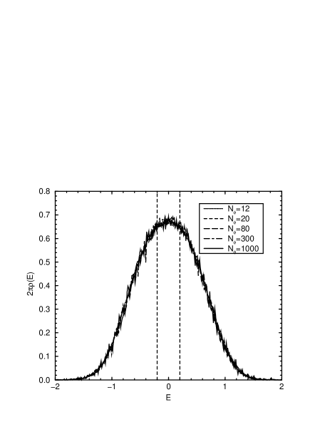
FIG. 5.: The density of states for a coupling $t=0.1$ between the two layers. $n_{p}=3N_{\phi}$ random pinning centers, modeled as random sign $\delta$-functions, were used in the calculation. The position of the pinning centers was taken to be random and independent in the two layers. The two dashed lines indicates the position of the two degenerate Landau levels in the absence of any disorder.

FIG. 6.: The Thouless number, $g_{s}$, for a coupling $t=0.1$ between the two layers. $n_{p}=3N_{\phi}$ random pinning centers, modeled as random sign $\delta$-functions, were used in the calculation. The position of the pinning centers was taken to be random and independent in the two layers. The two dashed lines indicates the position of the two states in the absence of any disorder. The results corresponds to the density of states in Fig. 5

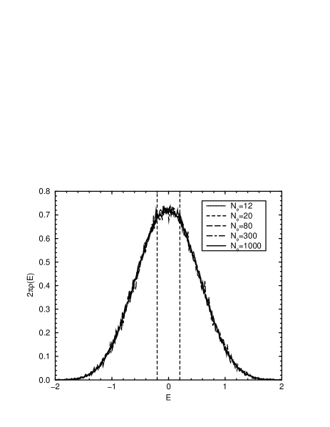
FIG. 7.: The density of states for a coupling $t=0.1$ between the two layers. $n_{p}=3N_{\phi}$ random pinning centers, modeled as random sign $\delta$-functions, were used in the calculation. The position of the pinning centers was taken to be random but the same in the two layers, corresponding to a form of correlated disorder. The two dashed lines indicates the position of the two degenerate Landau levels in the absence of any disorder.

FIG. 8.: The Thouless number, $g_{s}$, for a coupling $t=0.1$ between the two layers. $n_{p}=3N_{\phi}$ random pinning centers, modeled as random sign $\delta$-functions, were used in the calculation. The position of the pinning centers was taken to be random and but the same in the two layers, corresponding to a form of correlated disorder. The two dashed lines indicates the position of the two degenerate Landau levels in the absence of any disorder. The results corresponds to the density of states in Fig. 7

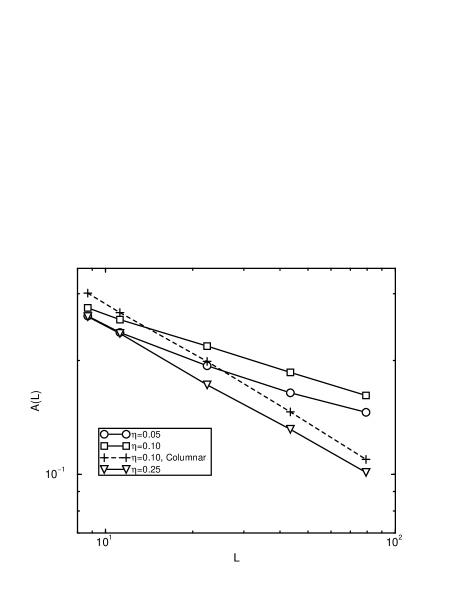
FIG. 9.: The integrated Thouless number as a function of $L$, for tunneling strenghts of $t=0.05,\ 0.1,\ 0.25$. The plusses denote results for $t=0.1$ with correlated disorder.

FIG. 10.: The reduced correlation length as a function of the energy $\gamma=\ln\sinh\theta$ for the double layer network model with a tunneling parameter of $\theta_{t}=0.05$.

FIG. 11.: Scaling collapse of the reduced correlation length for the double layer network model with a tunneling parameter of $\theta_{t}=0.05$.

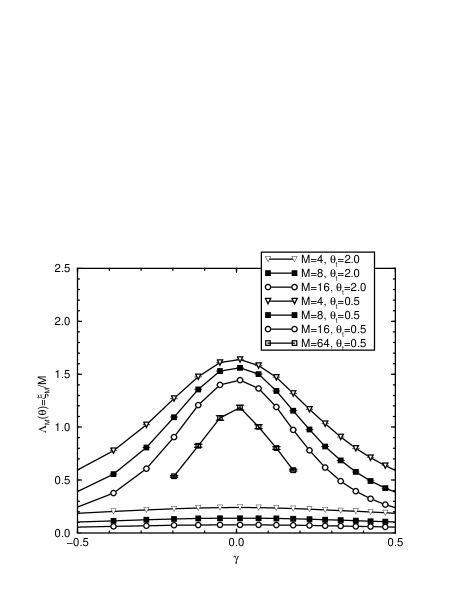
FIG. 12.: The reduced correlation length for two different values of $\theta_{t}=0.5$ and $2.0$. the results are for for the double layer network model.

- [1] D. E. Khmelnitskii, Pis’ma Zh. Eksp. Teor. Fiz. 38, 454 (1983) [JETP Lett. 38, 552 (1983)]; Helv. Phys. Acta 65, 164 (1992).
- [2] A. M. M. Pruisken, Phys. Rev. B 31, 416 (1985).
- [3] M. P. A. Fisher, Phys. Rev. Lett. 65, 923 (1990).
- [4] D. H. Lee, S. Kivelson, and S. C. Zhang, Phys. Rev. Lett. 68, 1375 (1992).
- [5] S. A. Trugman, Phys. Rev. B 27, 7539 (1983); S. Luryi and R. F. Kazarinov, Phys. Rev. B 27, 1386 (1983).
- [6] J. T. Chalker and P. D. Coddington, J. Phys. C 21, 2665 (1988).
- [7] G. V. Mil’nikov and M. Sokolov, Pis’ma Zh. Eksp. Fiz. 48, 494 (1988); JETP Lett. 48 536 (1988).
- [8] J. T. Chalker and G. J. Daniell, Phys. Rev. Lett. 61, 593 (1988).
- [9] S. Hikami, Phys. Rev. B 29, 3726 (1984); S. Hikami and E. Brézin, J. Phys. (Paris) 46, 2021 (1985); S. Hikami, Prog. Theor. Phys. 76, 1210 (1986).
- [10] R. R. P. Singh and S. Chakravarty, Nucl. Phys. BS265 [FS15], 265 (1986).
- [11] Y. Huo, R. E. Hetzel, and R. N. Bhatt, Phys. Rev. Lett. 70, 481 (1993).
- [12] D. Liu and S. Das Sarma, Phys. Rev. B 49, 2677 (1994).
- [13] H. Aoki and T. Ando, Sol. St. Comm. 38, 1079 (1981).
- [14] T. Ando, J. Phys. Soc. Jpn. 52, 1740 (1983).
- [15] H. Aoki and T. Ando, Phys. Rev. Lett. 54, 831 (1985).
- [16] T. Ando, Phys. Rev. B 40, 9965 (1989).
- [17] B. Huckestein and B. Kramer, Phys. Rev. Lett. 64, 1437 (1990).
- [18] Y. Huo and R. N. Bhatt, Phys. Rev. Lett. 68, 1375 (1992).
- [19] B. Huckestein, Rev. Mod. Phys. 67, 357 (1995).
- [20] B. Huckestein, Europhys. Lett. 20, 451 (1992).
- [21] H. P. Wei, and D. C. Tsui, M. A. Paalanen, and A. M. M. Pruisken, Phys. Rev. Lett. 61, 1294 (1988); A. M. M. Pruisken, Phys. Rev. Lett. 61, 1297 (1988).
- [22] S. Koch, R. J. Haug, K. v. Klitzing, and K. Ploog, Phys. Rev. B 43, 6828 (1991).
- [23] H. P. Wei, S. W. Hwang, D. C. Tsui, and A. M. M. Pruisken, Surf. Sci. 229, 34 (1990).
- [24] L. Engel, H. P. Wei, D. C. Tsui, and M. Shayegan, Surf. Sci. 229, 13 (1990).
- [25] L. W. Engel, D. Shahar, Ç. Kurdak, and D. C. Tsui, Phys. Rev. Lett. 71 2638 (1993).
- [26] This finding suggests that interaction effects must be important at some level since one would expect for truly non-interacting electrons.
- [27] S. W. Hwang, H. P. Wei, L. W. Engel, D. C. Tsui, and A. M. M. Pruisken, Phys. Rev. B 48, 11416 (1993).
- [28] H. W. Jiang, C. E. Johnson, K. L. Wang, S. T. Hannahs, Phys. Rev. Lett. 71, 1439 (1993).
- [29] K. Minakuchi, S. Hikami, Phys. Rev. B 53, 10898 (1996).
- [30] M. M. Fogler and B. I. Shklovskii, Phys. Rev. B 52, 17366 (1995).
- [31] D. E. Khmelnitskii, Phys. Lett. 106, 182 (1984); JETP Lett. 38, 556 (1983).
- [32] R. B. Laughlin, Phys. Rev. Lett. 52, 2304 (1984).
- [33] A. A. Shashkin, G. V. Kravchenko, and V. T. Dolgopolov, Pis’ma Zh. Eksp. Tero. Fiz. 58, 215 (1993) [JETP Lett. 58, 220 (1993)]; S. V. Kravchenko, W. Mason, J. .E. Furneaux, and V. M. Pudalov, Phys. Rev. Lett. 75, 910 (1995).
- [34] A. Glozman, C. E. Johnson, and H. W. Jiang, Phys. Rev. Lett. 74, 594 (1995).
- [35] T. V. Shahbazyan and M. E. Raikh, Phys. Rev. Lett. 75, 304 (1995).
- [36] K. Yang and R. N. Bhatt, Phys. Rev. Lett. 76, 1316 (1996).
- [37] D. Z. Liu, X. C. Xie, and Q. Niu, Phys. Rev. Lett. 76, 975 (1996).
- [38] T. Haavasoja, H. L. Störmer, D. J. Bishop, V. Narayanamurti, A. C. Gossard, and W. Wiegmann, Surf. Sci. 142 294 (1984).
- [39] H. L.Störmer, J. P. Eisenstein, A. C. Gossard, W. Wiegmann, and K. Baldwin, Phys. Rev. Lett. 56, 85 (1986).
- [40] S. E. Ulloa, Phys. Rev. Lett. 57, 2991 (1986).
- [41] C. A. Hoffman, J. R. Meyer, and F. J. Bartoli, J. Vac. Sci. Technol. B, 905 (1992).
- [42] H. L.Störmer, J. P. Eisenstein, A. C. Gossard, K. Baldwin, and J. H. English in 18th international conference on the physics of semiconductors Stockholm, Sweden, World Scientific, Singapore (1987), p. 385.
- [43] S. S. Murzin, Pis’ma Zh. Eksp. Fiz. 44, 45 (1986); JETP Lett. 44 56 (1986).
- [44] I. Laue, O. Portugal, and M. v. Ortenberg, Acta Phys. Pol. A 79, 359 (1991).
- [45] U. Zeitler, A. G. M. Jansen, P. Wyder, and S. S. Murzin, J. Phys. Cond. Matt. 6, 4289 (1994).
- [46] Y. J. Wang, B. D. McCombe, R. Meisels, F. Kuchar, and W. Schaff, Phys. Rev. Lett. 75, 906 (1995).
- [47] L. P. Gor’kov and A. G. Lebed’, J. Phys. Lett. 45, L-433 (1984).
- [48] L. Balents and M. P. A. Fisher, Phys. Rev. Lett. 76, 2782 (1996).
- [49] D. Poilblanc, G. Montambaux, M. Héritier, and P. Lederer, Phys. Rev. Lett. 58, 270 (1987); K. Machida, Y. Hasegawa, M. Kohmoto, V. M. Yakovenko, Y. Hori, and K. Kishigi, Phys. Rev. B 50 921 (1994); Y. Hasegawa, Phys. Rev. B 51, 4306 (1995).
- [50] U. M. Scheven, E. I. Chashechkina, A. Lee, and P. M. Chaikin, Phys. Rev. B 52, 3484 (1995); S. K. McKernan, S. T. Hannahs, U. M. Scheven, G. M. Danner, and P. M. Chaikin, Phys. Rev. Lett. 75, 1630 (1995); L. Balicas, G. Kriza, and F. I. B. Williams, Phys. Rev. Lett. 75, 2000 (1995).
- [51] T. Ohtsuki, B. Kramer, Y. Ono, Sol. State. Comm. 81, 477 (1992).
- [52] M. Henneke, B. Kramer, T. Ohtsuki, Europhys. Lett. 27, 389 (1994).
- [53] T. Ohtsuki, B. Kramer, Y. Ono, J. Phys. Soc. Jpn. 62, 224 (1993).
- [54] See B. Kramer and A. MacKinnon, Rep. Prog. Phys. 56, 1469 (1993) and references therein.
- [55] J. T. Chalker and A. Dohmen, Phys. Rev. Lett. 75, 4496 (1995).
- [56] T. Ohtsuki, Y. Ono, and B. Kramer, Surf. Sci. 263, 134 (1992).
- [57] D. K. K. Lee and J. T. Chalker, Phys. Rev. Lett. 72, 1510 (1994); D. K. K. Lee, J. T. Chalker, and D. Y. K. Ko, Phys. Rev. B 50 5272 (1994).
- [58] Z. Wang, D.-H. Lee, and X.-G. Wen, Phys. Rev. Lett. 72, 2454 (1994).
- [59] C. B. Hanna, D. P. Arovas, K. Mullen, and S. M. Girvin, Phys. Rev. B 52, 5221 (1995).
- [60] D. G. Polyakov and M. E. Raikh, Phys. Rev. Lett. 75, 1368 (1995).
- [61] K. Yang, K. Moon, L. Zheng, A. H. MacDonald, S. M. Girvin, D. Yoshioka, and S.-C. Zhang, Phys. Rev. Lett. 72, 732 (1994).
- [62] K. Moon, H. Mori, K. Yang, S. M. Girvin, A. H. MacDonald, L. Zheng, D. Yoshioka, and S.-C. Zhang, Phys. Rev. B 51, 5138 (1995).
- [63] K. Yang, K. Moon, L. Belkhir, H. Mori, S. M. Girvin, A. H. MacDonald, L. Zheng, and D. Yoshioka, submitted to Phys. Rev. B.
- [64] J. Hu and A.H. MacDonald, Phys. Rev. B 46, 12554 (1992).
- [65] S. Luryi, R. F. Kazarinov, Phys. Rev. B 27, 1386 (1983).
- [66] A. M. Tikofsky and S. A. Kivelson, unpublished, cond-mat/9507077. In this work interactions play an essential role.
- [67] L. W. Wong, H. W Jiang, N. Trivedi, E. Palm, Phys. Rev. B 51, 18033 (1995).
- [68] T. Wang, K. P. Clark, G. F. Spencer, A. M. Mack, and W. P. Kirk, Phys. Rev. Lett. 72, 709 (1994).
- [69] R. J. F. Hughes, J. T. Nicholls, J. E. F. Frost, E. H. Linfield, M. Pepper, C. J. B. Ford, D. A. Ritchie, G. A. C. Jones, E. Kogan, and M. Kaveh, J. Phys. Cond. Matt. 6, 4763 (1994).
- [70] D. G. Polyakov and B. I. Shklovskii, Phys. Rev. Lett. 70, 3796 (1993).
- [71] A. H. MacDonald, H. C. A. Oji, and K. L. Liu, Phys. Rev. B 34, 2681 (1986).
- [72] F. Wegner, Z. Phys. B 51, 279 (1983); E. Brézin, D. J. Gross, and C. Itzykson, Nucl. Phys. B235[FS11], 24 (1984).
- [73] D. J. Thouless, Phys. Rev. Lett. 39, 1167 (1977); D. J. Thouless and M. E. Elzain, J. Phys. C 11, 3425 (1978);
- [74] J. T. Edwards and D. J. Thouless, J. Phys. C 5, 807 (1972); D. C. Licciardello and D. J. Thouless, J. Phys. C 8, 4147 (1975); D. C. Licciardello and D. J. Thouless, Phys. Rev. Lett. 35, 1475 (1975).
- [75] E. Akkermans and G. Montambaux, Phys. Rev. Lett. 70, 481 (1993).
- [76] Q. Niu, D. J. Thouless, Y.-S. Wu, Phys. Rev. B 31, 3372 (1985).
- [77] D. P. Arovas, R. N. Bhatt, F. D. M. Haldane, P. B. Littlewood, and R. Rammal, Phys. Rev. Lett. 60, 619 (1988).
- [78] D.-H. Lee, Phys. Rev. B 50, 10788 (1994); D.-H. Lee and Z. Wang, unpublished; D.-H. Lee and Z. Wang, Phil. Mag. Lett. 73 145 (1996).
- [79] A. W. W. Ludwig, M. P.A. Fisher, R. Shankar, and G. Grinstein, Phys. Rev. B 50, 7526 (1994).
- [80] D.-H. Lee, Z. Wang, and S. Kivelson, Phys. Rev. Lett. 70, 4130 (1993).
- [81] A. MacKinnon, J. Phys. C 13, L1031 (1980); J. L. Pichard and G. Sarma, J. Phys. C 14, L127 (1981); ibid L617 (1981); A. MacKinnon and B. Kramer, Phys. Rev. Lett. 47, 1546 (1981); Z. Phys. B 53, 1 (1983).
- [82] We are grateful to D. K. K. Lee for suggesting this check to us.
- [83] H. A. Fertig and B. I. Halperin, Phys. Rev. B 36, 7969 (1987); H. A. Fertig, Phys. Rev. B 38 996, (1988).
- [84] L. Jaeger, J. Phys. Cond. Matt. 3, 2441 (1991).
- [85] As pointed out in Ref. [84], and later in Ref. [80], a fixed point described by classical percolation is only present in the network models if the intra-layer tunneling parameter, , is allow to be random. In our model we have taken all the intra-layer tunneling parameters to be uniform and independent of the site and this classical fixed point is therefore not presen and this classical fixed point is therefore not present.
- [86] D. Schoenberg, Magnetic Oscillations in Metals, (Cambridge University Press, Cambridge, 1984).
- [87] M. Stone (ed.), The Quantum Hall Effect, Singapore ; River Edge, N.J. : World Scientific, c1992.
- [88] Although the system would not be a bulk three-dimensional metal, as pointed out in recent work by Balents et al., Ref. [48], and Chalker et al., Ref. [55], the chiral surface states can show an unusual anisotropic two-dimensional metallic behavior.