Cluster Analysis for Percolation on Two Dimensional Fully Frustrated System

Abstract

The percolation of Kandel, Ben-Av and Domany clusters for 2d fully frustrated Ising model is extensively studied through numerical simulations. Critical exponents, cluster distribution and fractal dimension of percolative cluster are given.

I Introduction

A 2d fully frustrated (FF) Ising model is a model with Ising spins $\pm 1$ where the interactions between nearest neighbor spins have modulus $J>0$ and sign $\pm 1$ (ferro / antiferromagnetic interactions) and where the signs are chosen in such a way that every plaquette (i.e. the elementary cell of square lattice) is frustrated, i.e. every plaquette has an odd number of -1 interactions so that the four spins of the plaquette cannot simultaneously satisfy all four interactions. In Fig.1.1 we give an example of such a deterministic interaction configuration. In a plaquette of the FF model we can have only one or three satisfied interactions. The FF model has an analytical solution [1] and a critical temperature at $T_{c}=0$.

Since single-spin dynamics for FF suffers critical slowing down, a fast cluster dynamics was introduced by Kandel, Ben-Av and Domany (KBD) in Ref.[2].

The KBD-clusters are defined by choosing stochastically on each plaquette of a checkerboard partition of a square lattice one bond configuration between the three shown in Fig.1.2.

The probability of choice depends on spins configuration on the plaquette and it is a function of temperature (correlated site-bond percolation [3]). When there is only one satisfied interaction the zero-bond configuration is chosen with probability one. When three interactions are satisfied the zero-bond configuration is chosen with probability $P_{0}=e^{-4J/(kT)}$ (where $k$ is the Boltzmann constant and $T$ the absolute temperature), the bond configuration with two parallel bonds on two satisfied interactions is chosen with probability $P_{1}=1-P_{0}$ and the third bond configuration has zero probability. Two sites are in the same cluster if they are connected by bonds. For sake of simplicity from now on we choice $J/(kT)=1/T$.

Ref.[2] has stimulated several works [4, 5] that pay attention mainly to dynamics and to number of clusters and clusters sizes. In [5] numerical simulations on relatively large FF lattice sizes (number of sites $N=60^{2}\div 120^{2}$) supported the idea that the KBD-clusters represent spin correlated regions (like Coniglio-Klein clusters [6] do in Ising model) and consequently percolation temperature $T_{p}$ coincides with critical temperature $T_{c}$, percolation exponents coincide with critical ones and KBD-clusters at $T_{p}$ are 2d self-avoiding walks (SAW) at $\theta$ point. [7]

In this paper we extensively study percolative features of KBD-clusters, considering very large lattice sizes ($N=100^{2}\div 400^{2}$), and give numerical results on critical exponents, cluster distribution and fractal dimension at percolation point.

II Critical exponents and percolation point

We consider finite systems with increasing size ($L=100\div 400$) with periodic boundary conditions.

A cluster percolates when it connects two opposed system sides. For every size $L$ there is a percolation temperature $T_{p}(L)$. With $T_{p}$ (without any argument) we mean the percolation temperature in the thermodynamic limit i.e. $T_{p}(L)\rightarrow T_{p}$ for $L\rightarrow\infty$. In this limit percolating clusters are present at $T\leq T_{p}$ but not at $T>T_{p}$. In Fig.2 we show typical clusters at several temperatures for a finite system with size $L=60$.

For every $L$ we have studied the mean cluster size $S=\sum_{s}s^{2}n_{s}$ (where $s$ is the cluster size, $n_{s}$ the number of cluster of size $s$ per lattice site and the sum is extended over all finite clusters), the percolation probability $P=1-\sum_{s}sn_{s}$, the number of cluster $N_{c}=\sum_{s}n_{s}$, the number of bonds per lattice site $N_{b}$, the mean size of the largest (percolating) cluster $S_{I}$ and the mean size of the second largest (percolating) cluster $S_{II}$. These quantities are shown in Fig.3 for $L=100\div 400$. Let’s note that for $T\rightarrow 0$ the bonds cover 50% of lattice interactions (that is the random-bond percolation threshold on square lattice), $S_{II}$ goes to a finite value (like predicted by KBD [2] and already verified in Ref.[4]) and occupies almost 35% of the lattice, and that $S_{I}$ occupies almost 65% of the lattice. At $T=0$ only two clusters survive, as shown in Fig.2 e) and f).

Now we will give numerical estimates of critical exponents that characterize the KBD-cluster percolation.

We know [8] that in the thermodynamic limit the mean cluster size diverges for $T\rightarrow T_{p}$, the percolation probability goes to zero in the limit $T\rightarrow T_{p}^{-}$ and the number of cluster goes to zero for $T\rightarrow T_{p}^{+}$.

We assume that near $T_{p}$ the connectivity length $\xi$ (i.e. the typical linear cluster size) diverges like $\xi\sim|e^{-2/T}-e^{-2/T_{p}}|^{-\nu}$ , the mean cluster size diverges like $S\sim|e^{-2/T}-e^{-2/T_{p}}|^{-\gamma}$, the percolation probability goes to zero like $P\sim|e^{-2/T}-e^{-2/T_{p}}|^{\beta}$ and the number of cluster goes to zero like $N_{c}\sim|e^{-2/T}-e^{-2/T_{p}}|^{2-\alpha}$. The last relations are definitions of critical exponents $\alpha$, $\beta$, $\gamma$ and $\nu$.

By standard finite-size scaling considerations [8] we can make the ansatz

$$S\sim L^{\gamma/\nu}f_{S}(|e^{-2/T}-e^{-2/T_{p}}|L^{1/\nu})$$ (1)

$$P\sim L^{-\beta/\nu}f_{P}(|e^{-2/T}-e^{-2/T_{p}}|L^{1/\nu})$$ (2)

and

$$N_{c}\sim L^{(\alpha-2)/\nu}f_{N_{c}}(|e^{-2/T}-e^{-2/T_{p}}|L^{1/\nu})$$ (3)

where $f_{S}(x)$, $f_{P}(x)$ and $f_{N_{c}}(x)$ are universal functions, i.e. independent by $L$.

Via data-collapse (see Fig.4) we estimate the parameters $e^{-2/T_{p}}=0.0000$, $\alpha=0.1$, $\beta=0.00$, $\gamma=2.00$, and $\nu=1.00$ with error of one unit in the last given digit . Therefore the scaling relation $\alpha+2\beta+\gamma=2$ and the hyperscaling relation $2-\alpha=\nu d$ are satisfied with good approximation.

In Tab.1 we give numerical estimates of $T_{p}(L)$. The data are obtained taking for $L=100,200,300,400$ the values of $T_{p}(L)$ at which the $S$ data in a log-log plot vs. $|e^{-2/T}-e^{-2/T_{p}(L)}|$ follow two parallel straight lines (one above and one below $T_{p}(L)$) with slopes in good agreement with $\gamma=2$ and then best-fitting these values as $e^{-2/T_{p}(L)}\sim 1/L$.

III Fractal dimension and cluster distribution

Let’s now consider the fractal dimension $D$ of the percolating cluster. From the scaling invariance hypothesis [8] we know that $P\sim\xi^{D-d}$, then we obtain $D=d-\beta/\nu$ (hyperscaling). In present case we have $\beta=0$, then $D=d=2$. The same result is obtained from the scaling relation $\beta+\gamma=D\nu$.

This is confirmed by the analysis of cluster distribution (see Fig.5). The scaling invariance hypothesis [8, 9] gives for $T\rightarrow T_{p}$ and $s\rightarrow\infty$

$$n_{s}=s^{-\tau}f_{n_{s}}(|e^{-2/T}-e^{-2/T_{p}}|s^{\sigma})$$ (4)

with $\tau=1+d/D$, $\sigma=1/(\nu D)$ and $f_{n_{s}}(x)$ universal function.

From data-collapse for $n_{s}$ near $T_{p}$ (see Fig.6.a) we obtain numerical estimates of parameters. The data in Fig.6.a are chosen in such a way that the quantity $(e^{-2/T}-e^{-2/T_{p}})L^{1/\nu}$ (with $e^{-2/T_{p}}=0$ and $\nu=1$) is a constant with $T\simeq T_{p}(L)$ for every considered $L$. The results are $\tau=2.00$ and $\sigma=0.50$ (with error of one unit in the last digit), that, with the definitions of $\tau$ and $\sigma$, give $D=2$ and $\nu=1$. On the other hand these values of $\tau$ and $\sigma$ satisfies the relation $\sigma(2-\alpha)=\tau-1$, $\sigma\beta=\tau-2$, $\sigma\gamma=3-\tau$.[8]

From Fig.6.a we see that the universal function $f_{n_{s}}(x)$ is a bell-shaped curve for $T\simeq T_{p}(L)$. For temperatures slightly below $T_{p}(L)$ (Fig.6.b) $f_{n_{s}}(x)$ is shifted, while for temperatures slightly above $T_{p}(L)$ (Fig.6.c) $f_{n_{s}}(x)$ changes dramatically its shape.

Away from $T_{p}(L)$ we know [8] that is valid the relation

$$\log n_{s}\sim-s^{\zeta}$$ (5)

for $s\rightarrow\infty$, with $\zeta=1$ above $T_{p}(L)$ and $\zeta=1-1/d=1/2$ below $T_{p}(L)$. This relation is confirmed with reasonable approximation by our numerical simulations, as shown in Fig.7. Let’s note that, while the exponent $\zeta=1$ above $T_{p}(L)$ is good for a wide range of $s$ ($s=2000\div 8000$ for $L=100$), the exponent $\zeta=1/2$ below $T_{p}(L)$ is good for a smaller $s$ range ($s=2000\div 4400$ for $L=100$) since finite-size effect become more important below $T_{p}(L)$. The smaller $T$, the smaller $s$ range is.

A direct way to estimate the fractal dimension $D$ is given through its definition

$$s\sim R^{D}$$ (6)

for $T=T_{p}$, with $R$ radius of gyration of the cluster of size $s$. We know [8] that cluster dimension deviates from $D$ away from $T_{p}$, becoming the Euclidean dimension $d$ below $T_{p}$ and a value smaller than $D$ above $T_{p}$. This is true because eq.(6) is valid within the connectivity length $\xi$ for all temperatures, but $\xi$ goes to zero away from $T_{p}$. Unfortunately data about this relation are difficult to analyze. Indeed near $T_{p}(L)$ for every finite system with $L\leq 120$ it seems that $D$ is almost $7/4=1.75$ (the fractal dimension of a SAW at $\theta$ point), but for larger $L$ (see Fig.8 and Tab.1) the fractal dimension $D$ grows slowly to the asymptotic value 2.

IV Conclusions

We have numerically investigated the KBD-cluster percolation problem in 2d FF Ising model. From our simulation we found that, within numerical errors, this correlated site-bond percolation satisfies scaling and hyperscaling relations and have, in the thermodynamical limit, a percolation temperature $T_{p}=0$ and the exponents $\alpha=0$, $\beta=0$, $\gamma=2$, $\nu=1$, $\tau=2$, $\sigma=1/2$, $\zeta(T>T_{p}(L))=1$, $\zeta(T<T_{p}(L))=1/2$. Moreover at $T_{p}$ clusters are compact (fractal dimension $D=2$). Therefore now we can correct the conclusion of Ref.[5] and say that, since $T_{p}=T_{c}$ and $\nu$ is equal to spin correlation exponent [10], the site connectivity length $\xi$ goes like the spin correlation length diverging at zero temperature. Although the exponent $\gamma$ is different the coincidence between $\xi$ and correlation length is enough to give an efficient Monte Carlo cluster dynamics.[11]

TABLE I.: Numerical estimates of $T_{p}(L)$ and $D(L)$ for $L=60\div 400$. The way used to evaluate $T_{p}(L)$ and $D(L)$ give us confidence only on digit not in parentheses.

$L$	60	80	100	120	200	300	400
$T_{p}(L)$	0.51(7)	0.48(1)	0.45(6)	0.43(7)	0.39(2)	0.36(1)	0.34(2)
$D(L)$	1.7(2)	1.7(5)	1.7(7)	1.7(9)	1.8(2)	1.8(5)	1.8(6)

FIG. 1.: 1) Example of 2d FF lattice: the spin are on the vertices; solid lines represent ferromagnetic interactions ($+J$) and dashed lines antiferromagnetic interactions ($-J$). 2) Plaquette bond configurations: a) zero bond; b) two parallel vertical bonds; c) two parallel horizontal bonds.

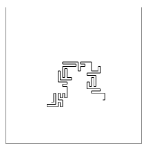
a b

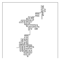
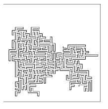
c d

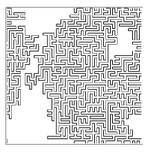
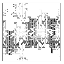
e f

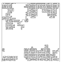
FIG. 2.: Typical KBD-clusters on a FF lattice with size $L=60$ with periodic boundary conditions: a) at $T=1$; b) at $T=0.65$; c) at $T=0.53$ slightly above $T_{p}(L)\simeq 0.52$; d) at $T=0.52\simeq T_{p}(L)$; e) at $T\simeq 0$ (largest cluster); f) at $T\simeq 0$ (the second cluster).

FIG. 3.: Mean cluster size $S$, percolation probability $P$, number of cluster $N_{c}$, number of bonds per lattice site $N_{b}$, mean size of largest cluster $S_{I}$ and mean size of second largest cluster $S_{II}$ vs. temperature $T$ for lattice sizes $L=100,200,300,400$. The error bars (often included in symbols) are the statistical errors.

FIG. 4.: Scaling for $S$, $P$ and $N_{c}$ following assumptions (1), (2) and (3) for data of systems with sizes $L=100,200,300,400$. The parameters $e^{-2/T_{p}}=0.0000\pm 0.0001$, $\alpha=0.1\pm 0.1$, $\beta=0.00\pm 0.01$, $\gamma=2.00\pm 0.01$ and $\nu=1.00\pm 0.01$ are such that the data for different sizes $L$ collapse on single curves (one for each graph). These curves are, respectively, the universal functions $f_{S}$, $f_{P}$ and $f_{N_{c}}$. The errors are estimated observing the range of parameters within which the data points collapse roughly well.

FIG. 5.: Cluster distribution $n_{s}$ vs. cluster size $s$ for a system with size $L=100$ at several temperatures $T$. Every bin is large 400 unities in cluster size. The percolation temperature for this system size is $T_{p}(L=100)\simeq 0.46$ then for all $T\geq 0.47$, even if the highest bin is not empty, there are only no percolating clusters. Let’s note that for all $T$ above $T_{p}(L)$ it is $n_{s}\sim e^{-s}$ and that the distribution become symmetric for $T\rightarrow 0$.

FIG. 6.: a) Scaling for $n_{s}$ following assumption (4) with parameter $\tau=2.00\pm 0.01$ and $\sigma=0.50\pm 0.01$ for data of systems with sizes $L=100,200,300,400$. Each set of data is chosen at a temperature near the corresponding $T_{p}(L)$. As consequence for each temperature the quantity $(e^{-2/kT}-e^{-2/T_{p}})L^{1/\nu}$ with $T_{p}=0$ and $\nu=1$ is equal to 2.084. Every point in the graph is an average over 500 consecutive values of $s$ for $L=100$, 2000 for $L=200$, 4500 for $L=300$, 8000 for $L=400$. b) As in part a) but for $(e^{-2/T}-e^{-2/T_{p}})L^{1/\nu}=0.823$ (below $T_{p}(L)$). c) As in part a) but for $(e^{-2/T}-e^{-2/T_{p}})L^{1/\nu}=3.567$ (above $T_{p}(L)$).

FIG. 7.: Fit of $\log(-\log n_{s}L^{2})$ vs. $\log(s/400)$ for a system with $L=100$ and $T_{p}(L)\simeq 0.46$: a) at $T\simeq 0.47>T_{p}(L)$ the slope is $\zeta\simeq 1$; b) at $T\simeq 0.45<T_{p}(L)$ the slope is $\zeta\simeq 1/2$.

FIG. 8.: Estimate of $D$ from definition (6) vs. $1/L$ (see Tab.1): at $T=0.517$ for $L=60$, at $T=0.481$ for $L=80$, at $T=0.450$ for $L=100$, at $T=0.437$ for $L=120$, at $T=0.389$ for $L=200$, at $T=0.360$ for $L=300$ and at $T=0.343$ for $L=400$. The error bars are probably underestimated. The arrow heads for the asymptotic value of $D$.

REFERENCES

- [1] J.Villain, J. Phys. C 10, 1717 (1977); G.Forgacs, Phys. Rev. B 22, 4473 (1980).
- [2] D.Kandel, R.Ben-Av and E.Domany, Phys. Rev. Lett. 65, 941 (1990); D.Kandel and E.Domany, Phys. Rev. B 43, 8539 (1991).
- [3] A.Coniglio, H.E.Stanley and W.Klein, Phys. Rev. Lett. 42, 518 (1979).
- [4] W.Kerler and P.Rehberg, Phys. Rev. B 49, 9688 (1994); P.D.Coddington and L. Han, Phys. Rev. B 50, 3058 (1994);
- [5] V.Cataudella, G.Franzese, M.Nicodemi, A.Scala and A.Coniglio, Phys. Rev. Lett. 47, 381 (1994) and Il Nuovo Cimento 16D N.8, 1259 (1994).
- [6] A.Coniglio and W.Klein, J. Phys. A 13, 2775 (1980).
- [7] A.Coniglio, N.Jan,I.Maijd and H.E.Stanley, Phys. Rev. B 35, 3617 (1987); B.Duplantier and H.Saleur, Phys. Rev. Lett. 59, 538 (1987).
- [8] D.Stauffer, Introduction to Percolation Theory (Taylor & Francis, London, 1985).
- [9] M.D’Onorio De Meo, D.W.Heermann and K.Binder, J. Stat. Phys., 60, 585 (1990).
- [10] as for clusters of parallel spin in 2d Ising model (Ref.[6]).
- [11] V.Cataudella, G.Franzese, M.Nicodemi, A.Scala and A.Coniglio, in print on Phys. Rev. E (cond-mat/9604169)