Computer simulation of crystallization kinetics with non-Poisson distributed nuclei

Abstract

The influence of non-uniform distribution of nuclei on crystallization kinetics of amorphous materials is investigated. This case cannot be described by the well-known Johnson-Mehl-Avrami (JMA) equation, which is only valid under the assumption of a spatially homogeneous nucleation probability. The results of computer simulations of crystallization kinetics with nuclei distributed according to a cluster and a hardcore distribution are compared with JMA kinetics. The effects of the different distributions on the so-called Avrami exponent $n$ are shown.
Furthermore, we calculate the small-angle scattering curves of the simulated structures which can be used to distinguish experimentally between the three nucleation models under consideration.

[Simulation of crystallization kinetics]

• Institut für Festkörper- und Werkstofforschung Dresden, PF 27 00 16, D-01171 Dresden, Germany

1 Introduction

The properties of metallic glasses and other amorphous materials may be impaired by even small amounts of crystalline phases. Crystallization can also improve the properties of some amorphous materials, e.g. glass ceramics. So the understanding of the crystallization process is very important. The analysis of experimental data is often made within the framework of the Avrami theory [1, 2] by means of the Johnson-Mehl-Avrami equation, which gives a relation between the fraction of transformed (i.e. crystallized) material $\chi(t)$ and the time at constant temperature. An equivalent approach was made by Kolmogorov [3].
Both models are based on the following assumptions:

1. Crystallization is considered in an unlimited medium.

2. Nucleation of crystals begins at time $t=0$ and occurs in a non-crystallized region. The nucleation rate per unit volume, $\alpha(t)$, is assumed to be independent of the coordinates.

3. The growth of crystals ceases at the points of mutual impingements, whereas it continues unchanged elsewhere. Before they touch each other, the crystals have a geometrically similar and convex shape (the Avrami approach is restricted to spherical crystals).

4. The growth rate $v(t)$ in a given direction is the same for all crystals and depends only on time.
   

Based on these assumptions, one can derive the following exact relation:

$$\chi(t)=1-\exp{\left[-\int\limits_{0}^{t}\alpha(\tau)V(\tau,t)\mbox{d}\tau\right]}$$ (1)

where

$$V(\tau,t)=V_{0}\left[\int\limits_{\tau}^{t}v(t^{\prime})\mbox{d}t^{\prime}\right]^{3}\hskip 25.0pt.$$ (2)

$V_{0}$ is a form factor, in the case of spherical crystals $V_{0}=4\pi/3$. An integration of equation (1) is only possible by making specific assumptions about the time dependence of the nucleation rate $\alpha(t)$.
If both $v$ and $\alpha$ are independent of time (interface controlled growth and continuous nucleation), then

$$\chi(t)=1-\exp\left[-\frac{1}{4}V_{0}\alpha v^{3}t^{4}\right]\hskip 25.0pt.$$ (3)

If only the growth rate $v$ is constant and all crystals are formed simultaneously at $t=0$ with a mean number density $\beta$ (instantaneous nucleation), the resulting nucleation rate $\alpha(t)=\beta\delta(t)$ can be substituted into equation (1). In this case

$$\chi(t)=1-\exp\left[-\beta V_{0}v^{3}t^{3}\right]\hskip 25.0pt.$$ (4)

Avrami proposed that for a three-dimensional nucleation and growth process with constant or decreasing nucleation rate, the general relation

$$\chi(t)=1-\exp(-kt^{n})$$ (5)

should describe the crystallized volume fraction. Equation (5) is the so-called Avrami equation with the Avrami exponent $n$, where $3\leq n\leq 4$.
This equation is often used to analyse experimental data by means of a logarithmic plot, where $\ln\left\{-\ln[1-\chi(t)]\right\}$ is plotted versus $\ln(t)$. The slope of the resulting straight line is the Avrami exponent $n$, which describes crystallization kinetics. But if the previously mentioned assumptions are not exactly satisfied, the resulting Avrami exponents $n$ may be misleading. We study cases where some of the assumptions (i-iv) are violated and no analytical results for the crystallization kinetics are available.
If the chemical composition of the two phases involved in the transformation is different, the growth rate is diffusion controlled. In this case, the radii $r$ of spherical crystals grow according to

$$r(t^{\prime},t)=g\cdot\sqrt{t-t^{\prime}}$$ (6)

where $g$ is a constant and $t$ and $t^{\prime}$ are the observation and nucleation times, respectively. Substituting (6) into equation (1) leads to an Avrami-exponent $n$ with $1.5\leq n\leq 2.5$. But if continuous nucleation occurs, assumption (iv) is violated, as the growth rate decreases with increasing life time of the crystal. As a consequence, crystals nucleated at different times have different growth rates. In the Johnson-Mehl method, the growth law (6) allows “phantom crystals” (crystals that are nucleated in an already crystallized area) to outgrow the real crystal. Therefore, the crystallized volume fraction is overestimated.
The assumption (ii) has no physical reasons. In practice, nucleation may occur preferentially in certain macroscopic regions (e.g. grain boundaries), so that the nucleation probability becomes dependent on the coordinates [4].
Furthermore, the grains have to reach a critical size $r_{\rm crit}$ to start growing.This critical radius is determined by the free energy and the surface energy. Therefore, in a sphere of radius $r_{\rm crit}$ only one crystal can nucleate [4]. This also violates assumption (ii).
In the present paper the influence of non-uniformly distributed nuclei and critical radii on crystallization kinetics is studied by computer simulation. We use methods of stochastic geometry [5, 6, 7], namely the germ-grain models. The models are explained in section 2 and the simulation technique is pointed out in section 3. The results are presented in section 4.

2 The models

A germ-grain model is defined by a point field $P_{1},P_{2},...$ with density $\lambda$ and a series of grains $A_{1},A_{2},...$ with finite size. The complete model $A$ is formed by the union of the grains $A_{n}$ shifted to the points $P_{n}$. Due to the diversity of point fields and types of possible grains there is a great variety of germ-grain models. In our study, we always use spherical grains of radius $r_{i}$.
To model the pure JMA case with assumptions (i-iv) fulfilled, we use a Poisson model for the underlying point field. The two fundamental properties of this point field are:

• The number, $N(G)$, of points lying in an arbitrary region $G$ with volume $V(G)$ is a random variable. The probability $P$ of finding $n$ points in the region $G$ is given by the Poisson distribution

  $$P(N(G)=n)=\frac{[\lambda V(G)]^{n}}{n!}\exp[-\lambda V(G)]\quad n=1,2,...\hskip 25.0pt.$$ (7)

• Considering disconnected regions $G_{1},G_{2},...$, the numbers $N(G_{1}),N(G_{2}),...$ are independent random variables.

Germ-grain models with an underlying Poisson point field and overlapping grains are also called Boolean models. For these models it is possible to calculate the volume fraction $\chi_{\rm A}$ analytically [5, 6, 7, 8]:

$$\chi_{\rm A}=1-\exp[-\lambda\bar{V}(A)]\hskip 25.0pt.$$ (8)

Here, $\lambda$ is the number density of the Poisson point field and $\bar{V}(A)$ is the mean volume of the grains. Equation (8) is equivalent to equations (3 - 5) if the corresponding nucleation and growth laws are inserted.
To model a system with increased nucleation probability in certain regions, we use a cluster point field. The nuclei are distributed uniformly and independently within spheres of radius $R_{\rm cl}$. These spheres are distributed according to a Poisson point field with parameter $\lambda_{\rm par}$, the numbers of points within the spheres are Poisson distributed with mean value $N_{\rm cl}$. Hence, the density of the cluster point field is $\lambda_{\rm cl}=\lambda_{\rm par}N_{\rm cl}$.
An appropriate set of parameters for characterizing the cluster model is $(\lambda_{\rm cl},N_{\rm cl},c)$ where $c=2R_{\rm cl}/\bar{r}_{1}$. Here, $\bar{r}_{1}$ is the mean distance of the midpoints of neighbouring clusters given by [7]:

$$\bar{r}_{1}=\left(\frac{3}{4\pi}\right)^{1/3}\Gamma(4/3)\lambda_{\rm par}^{-1/3}\approx 0.554\lambda_{\rm par}^{-1/3}\hskip 25.0pt.$$ (9)

For $c\gg 1$ the point field approaches a Poisson point field of density $\lambda_{\rm cl}$.
A hard-core point field is used to force a certain minimum distance between the nuclei. The distance between any points of the model with density $\lambda_{\rm hc}$ is forbidden to be smaller than a given value $R_{\rm hc}$. The essential property of the structure is described by the packing fraction $p_{\rm hc}=4\pi/3R_{\rm hc}^{3}\lambda_{\rm hc}$. For $p_{\rm hc}\rightarrow 0$ the point field approaches a Poisson point field.
Neither for the cluster model nor for the hard-core model analytical expressions are known that describe the volume fractions.
The small-angle scattering intensity $I(q)$ per unit volume is given by [9]:

$$I(q)=4\pi\int\limits_{0}^{\infty}r^{2}[C_{\rm A}(r)-\chi^{2}_{\rm A}(r)]\frac{\sin(qr)}{qr}{\mathrm{d}}r\hskip 25.0pt.$$ (10)

To calculate the small-angle scattering intensities of the germ-grain models, the covariance $C_{\rm A}(r)$ of the systems is needed. This is the probability $P$ of two random points $\vec{r}_{1},\vec{r}_{2}$ with distance $r$ both lying in the region covered by the model:

$$C_{\rm A}(r)=P(\vec{r}_{1}\in A,\vec{r}_{2}\in A)\>,\>r=\mid\vec{r}_{1}-\vec{r}_{2}\mid\hskip 25.0pt.$$ (11)

For Boolean models an analytical expression [8] exists:

$$C_{\rm A}=2\chi_{\rm A}-1+(1-\chi_{\rm A})^{2}\exp\left[\lambda\gamma^{0}(r)\right]$$ (12)

where $\gamma^{0}(r)$ is the mean distance probability function averaged over all spheres with density $f(x)$ of the radii distribution:

$$\gamma^{0}(r)=\frac{4\pi}{3}\int\limits_{r/2}^{\infty}x^{3}\left(1-\frac{3r}{4x}+\frac{r^{3}}{16x^{3}}\right)f(x){\mathrm{d}}x\hskip 25.0pt.$$ (13)

The constructional details of the point fields mentioned above are explained in the next section.

3 The simulation technique

The nucleation and growth processes are simulated in a cube of unit lenght $L_{0}$ and volume $V_{0}=L_{0}^{3}$. All lengths are scaled to $L_{0}$. To model an infinite structure, periodic boundary conditions are applied. We use spheres of equal (instantaneous nucleation) or different (continuous nucleation) size as grains. They grow according to the specified growth law and nuclei are generated randomly according to the underlying point field. In the case of instantaneous nucleation (INST), all grains start growing at $t=0$. If continuous nucleation (CONT) is considered, in every evolutionary step ${\mathrm{d}}t$ a mean number of nuclei starts growing according to the nucleation rate $\alpha(t)$. In this case, the nuclei that are created in an already transformed area have to be ommitted.
After every time step, the volume fraction $\chi_{\rm A}$ of the system is calculated. Optionally, the covariance $C_{\rm A}(r)$ of the structure can be calculated at a given volume fraction.
In every simulation, 500 - 700 nuclei are generated. To limit the influence of statistical fluctuations, the whole procedure is repeated 10 - 40 times and the average of the relevant quantities is evaluated.

3.1 Construction of the point fields

In a first step of the simulation the underlying point field has to be created.
To generate a Poisson point field, the number $N_{\rm nu}$ of nuclei is drawn from a Poisson distribution with parameter $\lambda V_{0}$. Then $N_{\rm nu}$ points with cartesian coordinates equally distributed in $(0,L_{0})$ are created.
A cluster point field is build by a two-step procedure. First, a Poisson point field of parent points with parameter $\lambda_{\rm par}$ is created in $V_{0}$. In a second step, spheres of radius $R_{\rm cl}$ are attached to these parent points. In each of these spheres, another Poisson process with parameter $N_{\rm cl}$ is created. Omitting the parent points, the remaining nuclei obey a cluster distribution with density $\lambda_{\rm cl}=\lambda_{\rm par}N_{\rm cl}$.
To construct a hardcore point field, single points with equally distributed coordinates are generated subsequently. New points are accepted only if their distance to all existing points is greater than $2R_{\rm hc}$. This procedure is repeteated until the desired number of nuclei (Poisson deviated with parameter $\lambda_{\rm hc}V_{0}$) is reached.

3.2 Nucleation and growth

After the definition of the point fields, the time evolution of the system starts.
In the case INST, all predefined grains start growing at $t=0$. In every time step, their radii are calculated as $r(t)=\int_{0}^{t}v(\tau){\mathrm{d}}\tau$. All grains have the same size.
If continuous nucleation is simulated, in every time step $N_{\rm act}$ nuclei start growing. $N_{\rm act}$ is Poisson deviated with the parameter $\alpha(t){\mathrm{d}}t$. The radii of the grains are different now, depending on the life time $t_{i}$ of each individual grain $i$:

$$r_{i}(t_{i})=\int\limits_{0}^{t_{i}}v(\tau){\mathrm{d}}\tau\hskip 25.0pt.$$ (14)

3.3 Calculation of the volume fraction and the covariance

To calculate the volume fraction, a fine grid of $N_{\rm test}$ test points is constructed in the unit cube. The coordinates of these test points are determined using a quasi-random sequence according to Sobol [10, 11, 12]. The volume fraction is given by the number of test points $N_{\rm in}$ that lie within the area covered by the spheres:

$$\chi_{\rm A}=\frac{N_{\rm in}}{N_{\rm test}}\hskip 25.0pt.$$ (15)

To evaluate the covariance, the distances between all the test points are calculated. The numbers $N(r)$ of test points that lie within discrete distance intervalls between $r$ and $r+{\mathrm{d}}r$ are determined. Then, the covariance is given as

$$C_{\rm A}(r)=\frac{N_{\rm in}(r)}{N(r)}$$ (16)

where $N_{\rm in}(r)$ denotes the number of test points in the distance intervall $(r,r+{\mathrm{d}}r)$ that are covered by a sphere.
The small-angle scattering intensities can now be calculated according to equation (10). To solve the integral, we use a Fourier transfom method and fit a polynomial to the discrete values of $C_{\rm A}(r)-\chi_{\rm A}^{2}$ in order to obtain the function to be integrated.

3.4 Test of accuracy

Due to the finite and discrete nature of the simulation, two sources of systematic errors have to be considered:

• The size of the system (i.e. the number of grains) has to be large enough in order to describe an infinite system.

• In the simulation of CONT, the nucleation proceeds in small but finite time steps ${\mathrm{d}}t$.

In order to check the accuracy of the simulation, we performed calculations using the Poisson point field and compared the results for the volume fraction and the covariance with the exact equations (3) and (4), respectively.
In figure 1, the results of simulations in the case of instantaneous and continuous nucleation are shown. The simulations were performed 10 times with a step size ${\mathrm{d}}t=10$ (INST) resp. ${\mathrm{d}}t=1$ (CONT) and $5\cdot 10^{4}$ test points were used. An Avrami analysis by means of linear regression yielded an Avrami exponent $n=2.96$ for the simulation of instantaneous nucleation, which is in good agreement with the exact value $n=3$.
In the case of continuous nucleation, the value of the Avrami exponent is $n=3.95$, compared with the exact value $n=4$.
The simulated small-angle scattering intensities of instantaneous nucleation (parameters as above) at different volume fractions are shown in figure 2. Here, quantitative differences between the simulated values and the exact ones calculated according to (10), (12) and (13) occur, although the covariance values are in quite good agreement, see figure 3. In both cases, the same numerical integration method was used. Because of the multiplication of $C_{\rm A}(r)-\chi_{\rm A}^{2}$ by $r$ in equation (10), very small differences between the simulated covariance values and the exact ones at large r-values yield substantial differences after integration.
Hence, with the present accuracy of our method, only qualitative statements concerning the small-angle scattering curves are possible. But the main features of the scattering intensities at different volume fractions are represented properly. The curve with low volume fraction shows well-resolved maxima and minima as the single spheres are still nearly isolated. With increasing volume fraction, the amplitudes of the oscillations decrease, at $\chi_{\rm A}=0.9$ there are only weak ripples left.

Figure 1: Comparison of the simulated volume fractions ($\bullet$) with the exact JMA-equation (–) in the case of instantaneous nucleation (INST) and homogeneous nucleation (CONT). The error bars denote the standard deviation of the results. INST: $\lambda=500$, $v=0.002$, CONT: $\alpha=5$, $v=0.002$, ${\mathrm{d}}t=1$.

Figure 2: Comparison of the simulated small-angle scattering values (dashed lines) with exact results (solid lines) for Poisson distributed nuclei at different volume fractions. The parameter $a$ denotes the radius of the grains. $\lambda=500$.

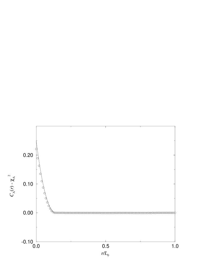
Figure 3: Comparison of the simulated covariance values ($\circ$) with exact results (–) according to (12). Parameters as in figure 1 (INST).

4 Results and discussion

We investigated the dependence of crystallization kinetics on the spatial distribution of the nuclei in the case of continuous nucleation (CONT) and instantaneous nucleation (INST). Additionally, for CONT the case of diffusion controlled growth was surveyed. The small-angle scattering intensities were calculated for instantaneous nucleation in order to check if it is possible to distinguish between the several grain distributions by means of small-angle scattering methods.

4.1 Instantaneous nucleation

In the case of instantaneous nucleation, we checked the influence of cluster- and hardcore-model on crystallization kinetics. The results were compared with the corresponding simulated values for the Poisson model. We used constant growth rates $v$ for calculations.
Furthermore, the covariance values and the resulting small-angle scattering intensities were evaluated.

4.1.1 Results on crystallization kinetics

In figure 4, Avrami plots of a cluster model and a hardcore model are compared with that of a Poisson model with equal point density $\lambda$. It is clearly shown that the distribution of the nuclei according to a cluster model leads to a reduced Avrami exponent $n$ compared with the value $n=3$ expected for the Poisson model. For small values of $c$, the simulated values deviate from a straight line in the Avrami plot, which means that the crystallization kinetics cannot be represented by an exponential law according to (5) in these cases. If $c$ is small enough, $n$ raises again and the deviations from the exponential law decrease again. The values of the simulated Avrami exponents (drawn from a linear regression analysis) are shown in table 1 for two simulations with ($\lambda_{\rm cl}=50,N_{\rm cl}=10,c$) and ($\lambda_{\rm cl}=25,N_{\rm cl}=20,c$), respectively.

Table 1: Avrami exponents for several parameter values of the cluster distribution and the hardcore model in case INST with $\lambda=500$. Poisson model: $n=2.97$

• Cluster, $N_{\rm cl}=10$			Cluster, $N_{\rm cl}=20$		Hardcore
  $c$	$n$	$c$	$n$	$p_{\rm hc}$	$n$
  2.66	2.36	2.11	2.08	0.26	3.56
  2.00	2.26	1.58	2.01	0.13	3.27
  1.33	2.26	1.06	2.07	0.06	3.07
  0.67	2.46	0.53	2.33	0.02	2.99
  0.33	2.43
  0.17	2.64
  0.08	2.80
  0.04	2.88

Simulation results in the case of a hardcore model with $\lambda_{\rm hc}=500$ and several hardcore radii $R_{\rm hc}$ are also listed. The simulation of the corresponding JMA case yields an Avrami exponent $n=2.97$. According to these simulation results, a distribution of the nuclei according to a hardcore model leads to an increased Avrami exponent $n$ compared with the one expected by the JMA theory. A deviation from the linear behaviour in the Avrami plot can also be observed for large values of $p_{\rm hc}$.

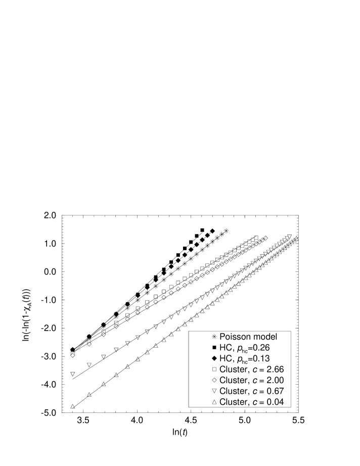
Figure 4: Influence of the parameter $c$ of the cluster model and the parameter $p_{\rm hc}$ of the hardcore model on the Avrami exponent in case INST. The straight lines are linear regression values. $\lambda=500,N_{\rm cl}=10$.

4.1.2 Results on small-angle scattering data

To check the possibility of distinguishing experimentally between the distributions under consideration, we investigated the small-angle scattering curves at several volume fractions.
The scattering curves of the Poisson model were already shown in figure 2. Figure 5 shows scattering curves of a germ-grain model with underlying hardcore distribution. For low volume fractions, the curves exhibit a significant first peak. This peak is characteristic for a hard-sphere model with non-overlapping spheres (see, e.g. [7]). With increasing volume fraction this peak disappears as the structure of the system is now far away from the structure of the generating nuclei and the overlapping of the grains becomes larger. The scattering curves of a cluster model with different volume fractions are shown in figure 6. Here, at low volume fractions no sharp peaks are present. With increasing volume fraction, the amplitude of the oscillations first increases and then decreases again.
Considering these results, it should be possible to distinguish between the three distributions of the nuclei by using small-angle scattering and observing the whole crystallization process.

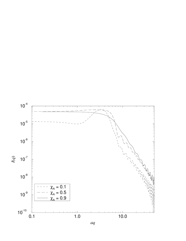
Figure 5: Simulated small-angle scattering curve of a harcore model with different volume fractions. $\lambda_{\rm hc}=500$, $R_{\rm hc}=0.045$. The parameter $a$ denotes the radius of the grains.

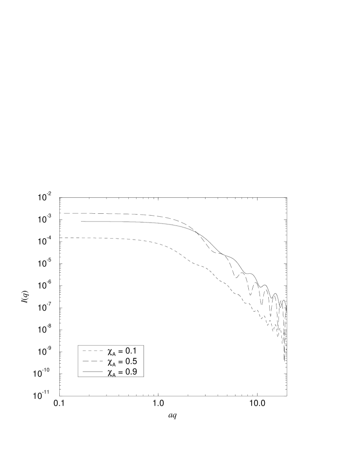
Figure 6: Simulated small-angle scattering curve of a cluster model with different volume fractions. $\lambda_{\rm cl}=50$, $N_{\rm cl}=10$, $c=2.0$. The parameter $a$ denotes the radius of the grains.

4.2 Continuous nucleation

The same investigations as in the case of instantaneous nucleation were also made for continuous nucleation and linear growth rate $v=\mbox{const.}$. In the case of diffusion controlled growth, we analysed the error that is made by applying the JMA equation.
In both cases, predefined point fields of density $\lambda=750$ and a nucelation rate $\alpha=5/{\mathrm{d}}t$ were used for the simulation.
In figure 7, the influence of a cluster and a hardcore point distribution on crystallization kinetics is shown (the given parameters describing the point fields refer to the predefined nuclei). Further simulation results are listed in table 2.

Table 2: Avrami exponents for several parameter values of the cluster distribution and the hardcore model in case CONT with $\alpha=5/{\mathrm{d}}t$. Poisson model: $n=3.95$

• Cluster, $N_{\rm cl}=10$			Cluster, $N_{\rm cl}=20$		Hardcore
  $c$	$n$	$c$	$n$	$p_{\rm hc}$	$n$
  4.57	3.72	3.63	3.56	0.27	4.04
  3.05	3.59	2.42	3.33	0.20	3.99
  1.52	3.40	1.21	3.14

As in the case of INST, a nuclei distribution according to the cluster model results in a decreased Avrami exponent compared with the JMA case and in deviations from the exponential behaviour. A hardcore distribution leads to an increased Avrami exponent, but the differences to the Poisson model are not as distinct as in case INST.

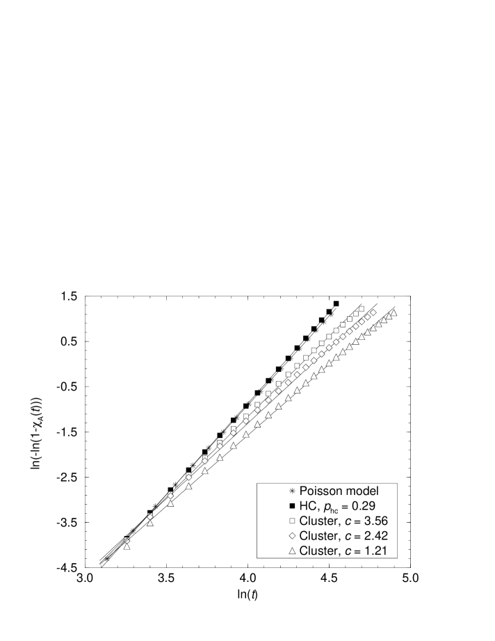
Figure 7: Influence of the parameter $c$ of the cluster model and the parameter $p_{\rm hc}$ of a hardcore model on the Avrami exponent in case CONT. The straight lines are linear regression values. $\lambda=750,N_{\rm cl}=20,\alpha=5/{\mathrm{d}}t$.

4.3 Discussion of crystallization kinetics

The deviations from the Poisson model in the cases INST and CONT can be explained by looking at the derivation of the JMA equation (see, e.g. [4]). To calculate the transformed volume fraction, a so-called extended volume is introduced, which is simply the sum of the volumes of all grains without considering their mutual overlappings. To get a connection between this extended volume and the real transformed volume, assumption (ii) is applied.
If the grains are distributed according to the cluster model, their overlapping is underestimated by the JMA model and hence the transformed volume fraction is overestimated. For $c\gg 1$ (clusters lose their cluster-like nature), $n$ is close to the JMA-value. With decreasing $c$ of the underlying cluster point field, the Avrami exponent $n$ gets smaller and substantial deviations from the exponential behaviour of the JMA-kinetics occur. If $c\rightarrow 0$, the Avrami exponent increases again and the Avrami plot shows a linear behaviour. In this case, the clusters are widely spaced and act like single Poisson-distributed nuclei. In between these two limiting cases ($c\gg 1$ and $c\rightarrow 0$), deviations from the JMA-behaviour occur. Values of $c$ with approximately $1<c<2$ give the maximum deviation (minimum $n$).
On the other side, a hardcore distribution leads to a smaller overlapping compared with a uniform distribution. The transformed volume fraction is larger than in the pure JMA case, since more of the space nuclei grow into is empty. Our simulations show an increase of the Avrami exponent $n$ with increasing packing fraction $p_{\rm hc}$ of the underlying point field. On the other hand, in the case of $p_{\rm hc}\rightarrow 0$ $n$ reaches the value of the pure JMA-case. Unfortunately, with our present algorithm we could not reach the limiting case of a close-packing of the underlying point field.
As outlined in section 1, in the case of diffusion controlled growth the crystallized volume fraction is overestimated. To check for this, we performed simulations with an underlying Poisson distribution of the nuclei. In a first series, the phantom nucleii that nucleated in an already crystallized region were discarded. Afterwards, they were treated like regular grains and contributed to the volume fraction. Doing so, we could estimate the error that is made in applying the JMA equation on diffusion controlled growth. The calculation of the differences $\Delta_{\rm abs}$ of the volume fractions yielded differences $\Delta_{\rm abs}\leq 9\cdot 10^{-3}$. These results are in good agreement with simulations made by Shepilov and Bochkarev [13].

5 Conclusions

Our simulations concernig the dependence of crystallization kinetics on the spatial nuclei distribution clearly showed that the analysis of experimental data by the JMA equation must be done with care. If the nuclei are not distributed equally, the use of the JMA equation can yield substantially wrong results. Therefore it should be checked if the JMA equation is applicable. One possibility to do so is the use of small-angle scattering. The scattering curves of the investigated nuclei distributions differ clearly from one another, especially in an early stage of the crystallization process.
On the other hand, the simulations showed that the error that is made by applying the JMA equation on diffusion controlled growth processes with continuous nucleation can be neglected.

References

References

- [1] Avrami M, J. Chem. Phys. 7, 1103 (1939).
- [2] Johnson W A and Mehl A, Trans. Am. Inst. Mining. Ing. 135, 416 (1939).
- [3] Shepilov M P and Baik D S, J. Non-Cryst. Solids 171, 141 (1994).
- [4] Christian J W, The Theory of Transformations in Metals and Alloys (Oxford Univ. Press, Oxford, 1985).
- [5] Stoyan D and Mecke J, Stochastische Geometrie. Eine Einführung. (Akademie-Verlag, Berlin, 1983).
- [6] Stoyan D, Kendall W S, and Mecke J, Stochastic Geometry and its Applications (Wiley & Sons, Chichester, 1987).
- [7] Hermann H, in Stochastic Models of Heterogeneous Materials, Materials Science Forum vol. 78, edited by G E Murch and F H Wöhlbier (Trans Tech Publications, Zürich, 1991).
- [8] Porod G, Kolloid-Z. 125, 51 (1952).
- [9] Sonntag U, Stoyan D, and Hermann H, Phys. Stat. Sol. (a) 68, 281 (1981).
- [10] Sobol I M, USSR Computational Mathematics and Mathematical Physics 7, 86 (1967).
- [11] Antonov I A and Saleev V M, USSR Computational Mathematics and Mathematical Physics 19, 252 (1979).
- [12] Press W H, Teukolsky S A, Vetterling W T, and Flannery B P, Numerical Recipes in FORTRAN: The Art of Scientific Computing (Cambridge University Press, Cambridge, 1992).
- [13] Shepilov M P and Bochkarev V B, Sov. Phys. Crystallogr. 32, 11 (1987).