Coherent patterns and self-induced diffraction of electrons on a thin nonlinear layer

The spontaneous formation of spatial structures (patterns) due to nonlinearity is well known for dissipative systems driven away from equilibrium. [2] In solid state physics those patterns have been mostly studied in the regime governed by classical macroscopic processes, [3] where quantum coherence effects were not important. In this paper we predict the spontaneous formation of quantum coherent non-dissipative patterns in semiconductor heterostructures with nonlinear properties.

Since the Schrödinger equation is linear, the nonlinearity appears in quantum systems due to the many-body effects and/or the coupling with the environment. In a mean-field approximation this problem can be traced to the self-consistent Schrödinger equation with the Hamiltonian $H=-\frac{\hbar^{2}}{2m}\nabla^{2}+V({\bf r})+V_{\rm eff}[|\psi({\bf r})|^{2}]$, where in addition to the external potential $V({\bf r})$ the self-consistent potential $V_{\rm eff}$ is introduced, representing a nonlinear response of the medium. [4] The potential $V_{\rm eff}$ depends on the probability $|\psi({\bf r})|^{2}$ of the carrier to be located at ${\bf r}$. When (in a weakly-nonlinear case) it is proportional to that probability, the resultant equation for a single-particle wave-function $\psi({\bf r})$ is the so-called nonlinear Schrödinger equation (NSE) with a cubic term [5] encountered in different contexts of the solid state physics: (i) the polaron problem, [6] where the strong electron-phonon interaction deformates the lattice thereby providing an attractive potential; [7] (ii) the magnetopolaron problem [8] in semimagnetic semiconductors, where the exchange interaction between the carrier spin and the magnetic impurities leads also to an effective attractive potential; [9, 10] (iii) Hartree-type interaction between electrons, giving a repulsive potential, [11] and others. [5]

Motivated by the great progress in heterostructure fabrication, some important results have been obtained recently in the framework of the cubic NSE for the situations when the nonlinearities are concentrated in thin semiconductor layers modeled by $\delta$-potentials. [9, 12, 13, 14] Among these results, we may mention the multiplicity of stable states found in different physical situations for which tunneling is important: an array of semimagnetic quantum dots, [9] a quantum molecular wire, [12] a doped superlattice formed by $\delta$-barriers. [13] Another is the oscillatory instability of the flux transmitted through the nonlinear layer. [14] It should be noted, however, that all these results are restricted to one-dimensional spatial supports, which means that the longitudinal and transverse degrees of motion are assumed to be decoupled. Disregarding that assumption in this paper, we show that considering additional spatial dimensions opens up the possibility of qualitatively new nonlinear phenomena – spontaneous formation of spatial transverse patterns, which are quantum-mechanically coherent.

Consider a thin layer in the $xy$-plane with the concentrated nonlinearity. We model the layer by using the $\delta$-function which simplifies greatly the calculations without modifying qualitatively the results. Keeping in mind possible pattern formation and analogy with the optics, the layer can be thought of as a screen. The steady-state scattering problem for the thin $\delta$-layer is governed by the NSE

$$-\frac{\hbar^{2}}{2m}\Delta\psi({\bf r})+(A+B|\psi({\bf r})|^{2})\;\delta(z)\;\psi({\bf r})=E\psi({\bf r}).$$ (1)

The external potential $A$ is allowed to be of the both signs, i.e., $A>0$ if it is a barrier and $A<0$ if it is a well. $B$ is the strength of the nonlinear potential: $B<0$ for the attractive and $B>0$ for the repulsive interaction. We do not specify the concrete physical model, because our results could be applicable to any of the above mentioned systems, although the most feasible candidates for the attractive case are believed to be semimagnetic heterostructures like CdTe/CdMnTe and CdTe/HgCdMnTe, where both, the height $A$ of the barrier and the strength $B$ can be varied by choosing the alloy composition. In addition, $A$ can be tuned by an external magnetic field. The expressions for $A$ and $B$ can be found elsewhere. [9] The repulsive case is an idealization of the situation considered in Ref. [11]; see Ref. [13].

We seek the solution in the form

$$\psi(x,y,z)=\left\{\begin{array}[]{lr}ae^{ikz}+b(x,y,z)\;e^{-ikz},&z<0\\ c(x,y,z)\;e^{ikz},&z>0\end{array}\right.$$ (2)

where the amplitude $a$ of the incident wave is fixed (real), and the electron energy $E=\frac{\hbar^{2}k^{2}}{2m}$. We assume that there is no current inflow along the screen (the only inflow into the system is from $z=-\infty$). Thus only those solutions satisfying the condition of zero inflow at $z$=0, $x,y\to\pm\infty$ will be considered.

It is convenient to write (2) and (1) in dimensionless form by means of the definitions: $\tilde{x}=\sqrt{2}kx,\tilde{y}=\sqrt{2}ky$, $\tilde{z}=kz$, $\tilde{b}=b/a$, $\tilde{c}=c/a$. Insertion of (2) into Equation (1) for $z\neq 0$ yields

$$\begin{array}[]{ll}\Delta_{\perp}\tilde{b}+\frac{1}{2}\,\partial_{\tilde{z}\tilde{z}}\tilde{b}-i\;\partial_{\tilde{z}}\tilde{b}=0,&\tilde{z}<0\\ \Delta_{\perp}\tilde{c}+\frac{1}{2}\,\partial_{\tilde{z}\tilde{z}}\tilde{c}+i\;\partial_{\tilde{z}}\tilde{c}=0,&\tilde{z}>0.\end{array}$$ (3)

By using the continuity of the wave-function $\psi$, one gets at $z$=0:

$$\partial_{\tilde{z}}\tilde{c}-\partial_{\tilde{z}}\tilde{b}+2i\;(\tilde{c}-1)=2(\alpha+\beta|\tilde{c}|^{2})\;\tilde{c},$$ (4)

and $\Delta_{\perp}\tilde{b}$=$\Delta_{\perp}\tilde{c}$. Here $\alpha$=$mA/(\hbar^{2}k)$ and $\beta$=$mBa^{2}/(\hbar^{2}k)$. Eqs. (3) and (4) have spatially uniform solutions $\tilde{c}$=$\xi+i\zeta$ such that $\zeta=-\alpha\xi-\beta\xi^{2}$, $|\tilde{c}|^{2}=\xi$, and

$$\beta^{2}\xi^{3}+2\alpha\beta\xi^{2}+(\alpha^{2}+1)\xi-1=0.$$ (5)

A straightforward analysis of this equation demonstrates that there is only one real root for $\alpha^{2}<3$ and there are three real roots under the conditions: $\alpha^{2}>3$, $\alpha\beta<0$, and $\beta^{-}<\beta<\beta^{+}$ with $\beta^{\mp}=\frac{2}{27}[\mp(\alpha^{2}-3)^{3/2}-\alpha^{3}-9\alpha]$. Thus multiple solutions are expected for two cases: the barrier ($\alpha>0$) with attractive nonlinearity ($\beta<0$) (case $\cal A$); the quantum well ($\alpha<0$) with repulsive nonlinearity ($\beta>0$) (case $\cal R$). Taking $\beta$ as a control parameter these solutions are depicted in Fig. 1 for different $\alpha$. Notice that we obtain up to three coexisting uniform solutions for different values of $\alpha$: $Z$-shaped curves $\xi(\beta)$ (if $\alpha>\sqrt{3}$) and $S$-shaped ($\sqrt{3}<\alpha<2$) or loop-shaped (if $\alpha>2$) curves $\zeta(\beta)$. At $\alpha$=2 there is a cusp of the maximum of the $\zeta(\beta)$ curve. The peaks in Fig. 1(a) correspond to maxima of the transmission for which $|\tilde{c}|^{2}$=$\xi$=1 and $\beta$=$-\alpha$. Since $\beta\propto a^{2}$, multiple solutions exist on a certain interval of incident wave amplitudes for any strength of the nonlinearity $B$. The threshold values $\alpha$=$mA/k\hbar^{2}$=$\pm\sqrt{3}$ for multiplicity of uniform solutions can be achieved by varying the barrier height (well depth) and/or the energy of the incident wave. Three uniform solutions coalesce at the tricritical parameter values: $\alpha_{0}$=$\pm\sqrt{3}$, $\beta_{0}$=$\mp 8\sqrt{3}/9$, $\xi_{0}$=3/4, $\zeta_{0}$=$\mp\sqrt{3}/4$. Hereafter we use the upper sign for case $\cal A$ and the lower sign for case $\cal R$.

We shall perform now a small-amplitude perturbation analysis of Eqs. (3) and (4) near the tricritical point. As a result we will find simple amplitude equations that will be solved in two particular cases of interest: (a) $y$-independent solutions, and (b) axisymmetric solutions.

Let $\alpha=\alpha_{0}\pm\delta$, $\beta=\beta_{0}\mp\gamma$ with $\delta>0$, $\gamma>0$ and $\delta,\gamma\ll 1$. We look for small nonuniform solutions: $\tilde{c}=\xi+i\zeta$, $\xi=\xi_{0}+\xi_{1}(\tilde{x},\tilde{y})$, $\zeta=\zeta_{0}+\zeta_{1}(\tilde{x},\tilde{y})$, where $\xi_{1}\ll\xi_{0}$, $\zeta_{1}\ll\zeta_{0}$. The richest distinguished limit corresponds to having $\gamma=\frac{4}{3}\delta+O(\delta^{3/2})$, $\xi_{1},\,\zeta_{1}=O(\sqrt{\delta})$, $\tilde{x},\,\tilde{y}=O(\delta^{-1/2})$, and $\tilde{z}=O(\delta^{-1})$. Inserting this Ansatz into Eqs. (3), the terms $\partial_{\tilde{z}\tilde{z}}\tilde{b}$ and $\partial_{\tilde{z}\tilde{z}}\tilde{c}$ are $O(\delta^{5/2})$ and can be ignored when compared with the others, which are $O(\delta^{3/2})$. Inserting the result into (4), we find

FIG. 1.: Real (a) and imaginary (b) parts of the transmitted amplitude $\tilde{c}$ as functions of $\beta$ for a uniform solution and different values of $\alpha$. Only case $\cal A$ is shown. The case $\cal R$ can be obtained by replacing $\alpha\to-\alpha$, $\beta\to-\beta$.

$$\partial_{\tilde{x}\tilde{x}}\xi_{1}+\partial_{\tilde{y}\tilde{y}}\xi_{1}=\frac{\delta}{\sqrt{3}}\;\xi_{1} - \frac{32}{27}\;\xi_{1}^{3}$$ (7)

$$+ \frac{\sqrt{3}}{4}\;(\frac{3}{4}\gamma-\delta)+O(\delta^{5/2}),$$ (9)

$$\zeta_{1}=\pm\xi_{1}/\sqrt{3}+O(\delta),$$

Notice that our Ansatz corresponds to weakly nonlinear perturbations of uniform solutions varying on a large spatial scale $\tilde{x}$=$\sqrt{2}kx=O(\delta^{-1/2})\gg 1$. The typical transverse length over which our solutions vary is thus much larger than the wavelength $1/k$.

With the substitutions: $\xi_{1}=\frac{3}{4}3^{1/4}\delta^{1/2}u$, $\tilde{x}=3^{1/4}\delta^{-1/2}X$, $\tilde{y}$=$3^{1/4}\delta^{-1/2}Y$, Eq. (7) can be written in the simpler form: $\partial_{XX}u+\partial_{YY}u=u-2u^{3}+\mu+O(\delta)$, $\mu=3^{-1/4}\delta^{-3/2}(\frac{3}{4}\gamma-\delta)=O(1)$. We report here only the results (for $y$-independent solutions and for the axisymmetric case) corresponding to the most symmetrical situation $\gamma=\frac{4}{3}\delta$ ($\mu$=0), where explicit formulas can be easily obtained. The results for the general non-symmetric case will be published elsewhere.

a Two-dimensional solutions depending on one transversal coordinate.

If $u$=$u(X)$ (two-dimensional solutions of the full problem depending on only one transversal coordinate), the parameter-free equation $\partial_{XX}u=u-2u^{3}$ can be integrated once yielding the result $(\partial_{X}u)^{2}=u^{2}-u^{4}+C$. This equation admits nonuniform solutions satisfying the condition of zero flux as $X\to\pm\infty$ only if $C$=0. In this case we obtain the solutions $u=\eta\;{\rm sech}(X-X_{0})$, with $\eta$=1 for the soliton and $\eta$=$-1$ for the antisoliton. Next we choose $X_{0}$=0. Finally, using relation (9) our solution for the transmitted and reflected amplitudes on the screen will be

$$\tilde{c}(\tilde{x}) = \frac{\sqrt{3}}{2}\;e^{\mp i\pi/6}[1+\sqrt{3}\eta\lambda\;{\rm sech}(\lambda\tilde{x})\;e^{\pm i\pi/3}],$$ (11)

$$\tilde{b}(\tilde{x}) = -\frac{1}{2}\;e^{\pm i\pi/3}[1-3\sqrt{3}\eta\lambda\;{\rm sech}(\lambda\tilde{x})\;e^{\mp i\pi/6}],$$ (12)

where $\lambda$=$3^{-1/4}\delta^{1/2}$ and the upper and lower signs refer to the cases $\cal A$ and $\cal R$, respectively. On the screen $z$=0 the difference between the cases $\cal A$ and $\cal R$ lies only in the phase of the wave function and not in the intensities: $|\tilde{c}(\tilde{x})|^{2}=\frac{3}{4}[1+\sqrt{3}\eta\lambda\;{\rm sech}(\lambda\tilde{x})]$, $|\tilde{b}(\tilde{x})|^{2}=\frac{1}{4}[1-3\sqrt{3}\eta\lambda\;{\rm sech}(\lambda\tilde{x})]$ (the small terms $\sim\lambda^{2}$ are dropped consistently with our scaling). The different phase factors give rise to drastic differences in the wave function outside the screen, as it will be shown below. We have also checked that the solutions are linearly stable when time evolution is considered subject to the boundary conditions discussed earlier.

The amplitudes of the transmitted and reflected waves outside the screen can be found from (3) using as the boundary conditions their values at $z$=0 and ignoring the small terms $\partial_{\tilde{z}\tilde{z}}\tilde{c}$ and $\partial_{\tilde{z}\tilde{z}}\tilde{b}$:

$$\tilde{c}(\tilde{x},\tilde{z})=\frac{1}{\sqrt{4\pi i\tilde{z}}}\int_{-\infty}^{\infty}\tilde{c}(\tilde{x}^{\prime},0)\;e^{i(\tilde{x}-\tilde{x}^{\prime})^{2}/(4\tilde{z})}\;d\tilde{x}^{\prime},$$ (13)

and the expression for $\tilde{b}(\tilde{x},\tilde{z})$ is the same once $\tilde{z}$ is replaced by $-\tilde{z}$.

In our 2D problem the intensities of the reflected and transmitted waves are nonuniform in space in contrast to the 1D problem, where they are constant. Denoting $|\tilde{c}(\tilde{x},\tilde{z})|^{2}=\Psi_{t}^{0}\{1+\Psi_{t}(\tilde{x},\tilde{z})\}$, $|\tilde{b}(\tilde{x},\tilde{z})|^{2}=\Psi_{r}^{0}\{1+\Psi_{r}(\tilde{x},\tilde{z})\}$, and using for $\tilde{c}(\tilde{x},0)$, $\tilde{b}(\tilde{x},0)$ the soliton-type solutions (a), we obtain $\Psi_{t}^{0}$=3/4, $\Psi_{r}^{0}$=1/4. The nonuniform parts of the intensities are given by

$$\Psi_{r,t} (\tilde{x},\tilde{z})=$$ (15)

$$\eta\frac{\sigma_{r,t}\lambda}{\sqrt{\pi|\tilde{z}|}}\int_{-\infty}^{\infty}\cos[\frac{(\tilde{x}-\tilde{x}^{\prime})^{2}}{4|\tilde{z}|}+\phi_{r,t}^{\pm}]\;{\rm sech}(\lambda\tilde{x}^{\prime})d\tilde{x}^{\prime}$$

where $\sigma_{r}$=$-3$, $\sigma_{t}$=$\sqrt{3}$, and the terms $\sim\lambda^{2}$ were dropped. The phase $\phi$ in the argument of cosine is different for the attractive and repulsive nonlinearities: (case $\cal A$): $\phi_{t}^{+}=\frac{1}{12}\pi$, $\phi_{r}^{+}=-\frac{5}{12}\pi$; (case $\cal R$): $\phi_{t}^{-}=-\frac{7}{12}\pi$, $\phi_{r}^{-}=-\frac{1}{12}\pi$.

Spatial distributions of the wave intensities are obtained by numerical integration of Eq. (15) and presented in Fig. 2 in terms of the scaled coordinates $X=\lambda\tilde{x}$, $Z=4\lambda^{2}\tilde{z}$. The off-screen wave intensities are shown starting from certain nonzero values of $Z$. The wave intensity on the screen is shown as a thin strip in the middle of Figs. 2(a),(b). The results can be interpreted as follows.

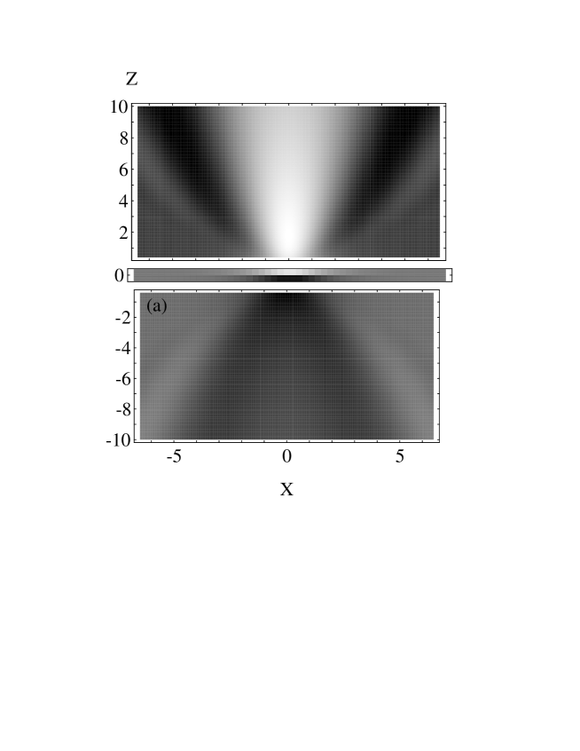
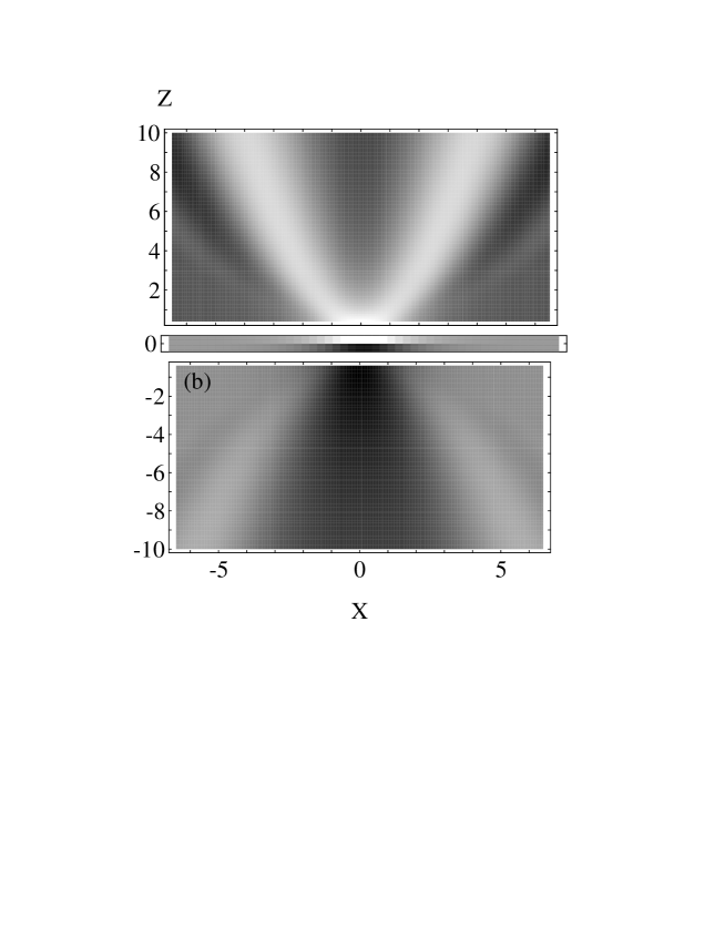
FIG. 2.: Density plots for the wave function intensities created by scattering off the self-induced nonuniform pattern on the screen at $Z$=0 with attractive (a) or repulsive (b) nonlinearities. White (black) color corresponds to the maximum (minimum) of the intensity for the soliton solution on the screen ($\eta=1$), and vice versa for the antisoliton solution ($\eta$=$-1$).

The uniform incident flow spontaneously produces a nonuniform soliton-type pattern on the screen and then is diffracted by it due to the nonlinear feedback in the equations. In particular, for the soliton solution ($\eta$=1) we observe local self-brightening of the transmitted wave with simultaneous local suppression of the reflected wave (Fig. 2). The diffraction pattern is crucially determined by the value of the phase factor $\phi^{\pm}$. For the case $\cal A$ the transmitted wave is focused into a “beam” of higher intensity with a maximum outside the screen at $Z\approx 1.7$ [Fig. 2(a)], whereas for the case $\cal R$ it is defocused and it “splits” into two “beams” [Fig. 2(b)]. Additional support for the importance of the phase factor is provided by the asymptotic behavior of the integral (15) in the remote zone $Z\gg 1$, $2X\ll Z$

$$\Psi_{r,t}(\tilde{x},\tilde{z})\approx\eta\;\sigma_{r,t}\sqrt{\frac{\pi}{|\tilde{z}|}}\cos(\frac{\tilde{x}^{2}}{4|\tilde{z}|}+\phi_{r,t}^{\pm}).$$ (16)

In the transverse direction the local maxima (minima) of the intensities are determined by the condition $\frac{\tilde{x}^{2}}{4|\tilde{z}|}+\phi_{r,t}^{\pm}=\pi m$, $m=0,\pm 1,\dots$. For instance $\phi_{t}^{+}>0$ for case $\cal A$, and the cosine in (16) reaches its maximum at $\tilde{x}$=0 providing a transmitted “beam” along the axes. $\phi_{t}^{-}<0$ for case $\cal R$, and the cosine is largest on the parabola $\tilde{z}=\frac{3}{7\pi}\tilde{x}^{2}$ yielding two transmitted “beams” as in Fig. 2(b). The behavior of the reflected wave is also nontrivial: for case ${\cal A}$ the reflected pattern contains “split traces”: the suppressed reflection forms the parabola $\tilde{z}=\frac{3}{5\pi}\tilde{x}^{2}$ [Fig. 2(a)], whereas for case ${\cal R}$ the reflection is suppressed within a single trace [Fig. 2(b)]. It should be noted, however, that for the antisoliton solution ($\eta$=$-1$) the maxima and minima are interchanged (with respect to the soliton solution), the “beams” become the suppressed traces and vice versa. Which type of solution (self-brightening or self-darkening of the transmission) will be realized in practice depends on additional conditions: type of the imperfections pinning the soliton, boundary conditions, past history, and so on.

b Two-dimensional axisymmetric solutions.

For this geometry, $u$=$u(R)$, $R^{2}=X^{2}+Y^{2}$, and the parameter-free equation becomes $\partial_{RR}u+\frac{1}{R}\partial_{R}u=u-2u^{3}$. There are infinitely many solutions which satisfy our boundary conditions $u(\infty)=0$ and $u_{R}(0)$=$u_{R}(\infty)$=0. We denote them by $S_{n}^{+}$ for the soliton case [$u(0)>0$] and $S_{n}^{-}$ for the antisoliton case [$u(0)<0$], where the subscript $n=0,1,\dots$ is the number of zeros of $S_{n}^{\pm}$ as shown in Fig. 3. Then $S_{n}^{-}$=$-S_{n}^{+}$.

In conclusion, spontaneous formation of spatial transverse patterns, which are quantum-mechanically coherent is expected to occur in semiconductor heterostructures with a thin nonlinear layer. Self-diffraction of the electron wave on the transverse patterns gives rise to interesting phenomena like self-brightening or darkening of the transmitted wave, beam splitting, etc.

This work has been supported by the DGICYT grants PB92-0248 and PB94-0375, and by the EU Human Capital and Mobility Programme contract ERBCHRXCT930413. O.M.B. acknowledges support from the Ministerio de Educación y Ciencia of Spain.

FIG. 3.: Axisymmetric solutions $S_{n}^{+}$ for the transmitted amplitude on the screen when n=1,2,3. Recall that $S_{n}^{-}$=$-S_{n}^{+}$.

REFERENCES

- [1] Present address: Dept. Física Fonamental, Universitat de Barcelona, Av. Diagonal 647, E-08028 Barcelona, Spain.
- [2] M. Cross and P. C. Hohenberg, Rev. Mod. Phys. 65, 851 (1993).
- [3] Nonlinear Dynamics and Pattern Formation in Semiconductors and Devices, edited by F.-J. Niedernostheide (Springer-Verlag, Berlin, 1995).
- [4] J. Callaway, Quantum Theory of the Solid State, 2nd. ed., (Academic, San Diego, 1991).
- [5] See, e.g., the review: V. G. Makhankov and V. K. Fedyanin, Phys. Rep. 104, 1 (1984), and references therein.
- [6] M. F. Deigen and S. I. Pekar, Sov. Phys. JETP, 21, 803 (1951); S. I. Pekar, Untersuchungen uber die Elektronentheorie der Kristalle (Akademie-Verlag, Berlin, 1954); V. A. Kochelap, V. N. Sokolov, and B. Yu. Vengalis, Phase Transitions in Semiconductors with Deformation Electron-Phonon Interaction, (Naukova Dumka, Kiev, 1984).
- [7] M. A. Smondyrev, P. Vansant, F. M. Peeters, and J. T. Devreese, Phys. Rev. B 52, 11231 (1995).
- [8] J. K. Furdyna, J. App. Phys. 64, R29 (1988).
- [9] P. Hawrylak, M. Grabowski, and J. J. Quinn, Phys. Rev. B 44, 13082 (1991).
- [10] C. Benoit à la Guillaume, Yu. G. Semenov, and M. Combescot, Phys. Rev. B 51, 14124 (1995).
- [11] C. Presilla, G. Jona-Lasinio, and F. Capasso, Phys. Rev. B 43, 5200 (1991); G. Jona-Lasinio, C. Presilla, and F. Capasso, Phys. Rev. Lett. 68, 2269 (1992); G. Jona-Lasinio, C. Presilla, and J. Sjöstrand, Ann. Phys. (NY) 240, 1 (1995).
- [12] L. I. Malysheva and A. I. Onipko, Phys. Rev. B 46, 3906 (1992).
- [13] N. G. Sun and G. P. Tsironis, Phys. Rev. B 51, 11221 (1995).
- [14] B. A. Malomed and M. Ya. Azbel, Phys. Rev. B 47, 10402 (1993).