The Ising-Kondo lattice with transverse field:
an $f$-moment Hamiltonian for URu₂Si₂?

Abstract

We study the phase diagram of the Ising-Kondo lattice with transverse magnetic field as a possible model for the weak-moment heavy-fermion compound URu₂Si₂, in terms of two low-lying $f$ singlets in which the uranium moment is coupled by on-site exchange to the conduction electron spins. In the mean-field approximation for an extended range of parameters, we show that the conduction electron magnetization responds logarithmically to $f$-moment formation, that the ordered moment in the antiferromagnetic state is anomalously small, and that the Néel temperature is of the order observed. The model gives a qualitatively correct temperature-dependence, but not magnitude, of the specific heat. The majority of the specific heat jump at the Néel temperature arises from the formation of a spin gap in the conduction electron spectrum. We also discuss the single-impurity version of the model and speculate on ways to increase the specific heat coefficient. In the limits of small bandwidth and of small Ising-Kondo coupling, we find that the model corresponds to anisotropic Heisenberg and Hubbard models respectively.
PACS numbers: 71.10.Fd, 71.27.+a, 71.70.Ch, 75.30.Mb

I Introduction

As the large specific heat jump of URu₂Si₂ at its Néel temperature of $T_{N}=17.5$ K is difficult to reconcile with its anomalously small staggered magnetization[1, 2], some authors[3, 4, 5] have speculated that there is some hidden order parameter. Recent neutron experiments indicate, however, that the weak Bragg peaks of the ordered phase break time reversal symmetry as would be the case if the order were magnetic dipolar[6]. In addition the hidden multispin order parameters proposed to account for the large specific heat jump have been shown to give the opposite field-dependence for the Bragg peaks to that observed in experiment [7]. To date, neither the small moments (about 1% of the full uranium moment[1, 2]) nor the large specific heat jump[8] $\Delta C/C\approx 1$ at $T_{N}$ have been explained. In this paper, we present a model which may account for the small moments, and discuss additional requirements needed to attain sufficiently large specific heat jump $\Delta C$ and linear specific heat coefficient $\gamma$.

The sharp, dispersive spin excitations in URu₂Si₂ are longitudinal, and are well described in terms of a transition between two crystal-field singlets[1, 2]; no sharp higher energy levels have been observed, consistent with the highly anisotropic susceptibility. The low transverse susceptibility ($\chi^{z}/\chi^{x,y}\sim 5$ as $T\to 0$) indicates that the next higher degenerate crystal-field levels are at energies an order of magnitude higher than the $\Delta=2.4$ THz of the first excited singlet state. A broad longitudinal continuum has been observed at higher energies, but we focus here on the sharp crystal-field-like features of the spectrum. Although a doublet crystal-field ground state has been proposed[9] for U diluted in ThRu₂Si₂ with its different cell parameters, we follow the evidence from neutron scattering that URu₂Si₂ has two low-lying singlets separated by a gap $\Delta$.

In an attempt to describe the magnetism of URu₂Si₂, we consider the following Hamiltonian which is an Ising-Kondo lattice model with transverse field:

$$H=\sum_{\vec{k}}\epsilon_{\vec{k}}^{\ }\psi^{\dagger}_{\vec{k}}\psi^{\ }_{\vec{k}}+I\sum_{i}S^{z}_{i}\psi^{\dagger}_{i}{\textstyle\frac{1}{2}}\sigma^{z}\psi^{\ }_{i}-\Delta\sum_{i}S^{x}_{i}$$ (1)

where $\psi^{\dagger}_{i}\equiv(c^{\dagger}_{i\uparrow},c^{\dagger}_{i\downarrow})$ (with $\psi^{\dagger}_{\vec{k}}$ as its Fourier transform), and $c^{\dagger}_{i\sigma}$ creates a conduction electron of spin $\sigma=\uparrow,\downarrow$ at lattice site $i$; $\epsilon_{\vec{k}}$ is the conduction band energy, with width $2W$. The $S=1/2$ operators $\vec{S}_{i}$, normalized so $\vec{S}_{i}^{2}=3/4$, correspond to the two-level system consisting of the two low-lying singlets which are separated by an energy $\Delta$, and we thus regard it as the spin operator for $f$ electrons: the isotropic Kondo exchange $I\sum_{i}\vec{S}_{i}\cdot(\psi^{\dagger}_{i}{\textstyle\frac{1}{2}}\vec{\sigma}\psi^{\ }_{i})$ reduces to the above Ising form when the true $f$-spin is projected onto the lowest two singlet states. Details about the crystal-field splitting are given in Appendix A.

In Ref. [[10]], parameters of this Hamiltonian were estimated that agreed with the expected 6$d$ conduction-electron bandwidth $2W\approx 500$ THz, on-site exchange $I\approx 25$ THz comparable to that in other heavy-fermion systems, and the singlet-singlet gap $\Delta\approx 2.4$ THz observed in neutron scattering at low T. These authors also reported an order-of-magnitude mass enhancement from spin fluctuations above $T_{N}$, but as discussed in Sec. IV, a lowest order perturbative calculation shows that the mass enhancement is small unless I/W is $O(1)$.

While URu₂Si₂ does not necessarily correspond exactly to half-filling, in this paper we restrict attention to the half-filled case, to one-dimensional (1D) and centred tetragonal[11] (ct) lattices, and a conduction-electron band constructed from inter-sublattice hopping:

$$\sum_{\vec{k}}\epsilon_{\vec{k}}^{\ }\psi^{\dagger}_{\vec{k}}\psi^{\ }_{\vec{k}}=-t\sum_{\langle ij\rangle,\sigma}c_{i\sigma}^{\dagger}c_{j\sigma}^{\ }+{\rm h.c.}$$ (2)

where $\langle ij\rangle$ denotes bonds between nearest neighbours on opposite sublattices. Specifically,

$$\epsilon_{\vec{k}}=\left\{\begin{array}[]{ll}-2t\cos(ka),&\mbox{1D}\\ -8t\cos(k_{x}a/2)\cos(k_{y}a/2)\cos(k_{z}c/2),&\mbox{{\sc ct}}\end{array}\right.$$ (3)

so that the bandwidth $2W$ is $4t$ ($16t$) in the 1D (ct) lattice. Here the conventional ct unit cell, considering the ct lattice to be bct, measures $a\times a\times c$.

This paper proceeds as follows. We study the model mainly in the mean-field approximation, and find an extensive low-moment regime as well as reasonable Néel temperature, although the specific heat, while showing a jump at $T_{N}$, is not of sufficient magnitude. Using a single-impurity model for the specific heat, we speculate on ways to obtain a large specific heat coefficient $\gamma$. We also find that in the limits of small bandwidth and low coupling, direct comparisons with other electron correlation models are possible.

II Mean-Field Approximation

We present mean-field results for our Hamiltonian which naturally provide a region of parameter space in which the required small moments occur.

Taking as our mean-field ansatz $S^{z}_{j}=(-1)^{j}m_{f}+\delta S^{z}_{j}$ for the $f$-electron spins and $\psi^{\dagger}_{j}{\textstyle\frac{1}{2}}\sigma^{z}\psi^{\ }_{j}\equiv s^{z}_{j}=(-1)^{j+1}m_{c}+\delta s^{z}_{j}$ for the conduction-electron spins, where $(-1)^{j}\equiv\exp(i\vec{Q}\cdot\vec{R}_{j})$ alternates between opposite sublattices, our Hamiltonian becomes, upon dropping the product of fluctuations,

$$H_{\rm MF} = \sum_{\vec{k}}(\psi^{\dagger}_{\vec{k}},\psi^{\dagger}_{\vec{k}+\vec{Q}})\!\left(\!\begin{array}[]{cc}\epsilon_{\vec{k}}&Im_{f}{\textstyle\frac{1}{2}}\sigma^{z}\\ Im_{f}{\textstyle\frac{1}{2}}\sigma^{z}&\epsilon_{\vec{k}+\vec{Q}}\end{array}\!\right)\!\left(\!\begin{array}[]{c}\psi^{\ }_{\vec{k}}\\ \psi^{\ }_{\vec{k}+\vec{Q}}\end{array}\!\right)$$ (9)

$$-\sum_{j}[(-1)^{j}Im_{c}S_{j}^{z}+\Delta S_{j}^{x}]+{\cal N}Im_{f}m_{c}\>\>,$$

where ${\cal N}$ is the number of uranium atoms, and $\vec{k}$ runs over the magnetic Brillouin zone. Minimizing the free energy, we obtain self-consistent mean-field equations for the $f$- and conduction-electron moments $m_{f}$ and $m_{c}$, given here for bands $\epsilon_{\vec{k}}$ satisfying the generalized nesting condition $\epsilon_{\vec{k}}=-\epsilon_{\vec{k}+\vec{Q}}$ for all $\vec{k}$ (which occurs, for example, for nearest-neighbour inter-sublattice hopping in 1D, square, and ct lattices):

$$m_{f} = {Im_{c}\over 2\tilde{\Delta}}\tanh(\beta\tilde{\Delta}/2)\>\>,$$ (10)

$$m_{c} = {Im_{f}\over{\cal N}}\sum_{\vec{k}}\frac{\tanh(\beta\tilde{\epsilon}_{\vec{k}}/2)}{2\tilde{\epsilon}_{\vec{k}}}\>\>,$$ (11)

where $\pm\tilde{\epsilon}_{\vec{k}}^{\ }\equiv\pm\sqrt{\epsilon_{\vec{k}}^{2}+({\textstyle\frac{1}{2}}Im_{f})^{2}}$ and $\tilde{\Delta}\equiv\sqrt{\Delta^{2}+(Im_{c})^{2}}$ are the mean-field energy levels, and $\beta$ is the inverse temperature. We note that the mean-field moments $m_{f}$ and $m_{c}$ both have mean-field critical exponent ${1\over 2}$ and are therefore proportional to each other near the Néel temperature $T_{N}$, which is obtained by the solution of

$$\coth(\Delta/2k_{B}T_{N})={I^{2}\over{\cal N}}\sum_{\vec{k}}{\tanh(\epsilon_{\vec{k}}/2k_{B}T_{N})\over 4\Delta\epsilon_{\vec{k}}}\>\>.$$ (12)

The specific heat per uranium atom is

$$C = \frac{k_{B}}{{\cal N}}\sum_{\vec{k}}\left[(\beta\tilde{\epsilon}_{\vec{k}})^{2}-\frac{I^{2}}{k_{B}^{2}8T}{\partial m_{f}^{2}\over\partial T}\right]{\rm sech}^{2}(\beta\tilde{\epsilon}_{\vec{k}}/2)$$ (14)

$$+{k_{B}\over 4}\left[(\beta\tilde{\Delta})^{2}-\frac{I^{2}}{2k_{B}^{2}T}{\partial m_{c}^{2}\over\partial T}\right]{\rm sech}^{2}(\beta\tilde{\Delta}/2)\>\>.$$

For comparison to experiment, we note that a staggered magnetization $m_{f}=0.5$ in our $S_{f}={\textstyle\frac{1}{2}}$ model corresponds to a true moment of 1.2$\mu_{B}$, as this is the observed matrix element of the true $S^{z}$ operator between the two singlets[2]. In Fig. 1 we show that small $f$-moments naturally arise from the mean-field approximation in a region of parameter space not too far from the values of Ref. [[10]] quoted above. Mean-field theory also gives a Néel temperature of appropriate order. We expect that in a full calculation fluctuation effects would reduce both the moments and Néel temperature. Thus the values of the parameters could differ from those derived by matching mean-field theory to experiment.

It is difficult within mean-field theory to obtain both the Néel temperature and moments of experiment since we do not have freedom to simply scale all parameters: the singlet-singlet spacing cannot be very different from $\Delta=2.4$ THz.

Since the Fermi surface is perfectly nested (in the generalized sense defined above) by the antiferromagnetic wave-vector — this is true for nearest-neighbour inter-sublattice hopping in 1D, square, and ct lattices — we find that, as expected, the conduction electrons exhibit logarithmic response to the field produced by the $f$-system: if $Im_{f}\ll W$, then $m_{c}\sim m_{f}|\log m_{f}|^{d}$ in $d$ dimensions. This behaviour is caused by the sharp corners found in the Fermi surface only at half-filling, and is therefore not present away from half-filling, or for more general Fermi surfaces.

The temperature-dependence of the $f$-moment and specific heat for selected parameters are given in Fig. 2 for the 1D case, showing a jump $\Delta C/C\approx 15$% with $C$ too small by a factor of 6 to fit experiment. The jump arises mainly from the formation of a spin gap $Im_{f}$ in the conduction electron spectrum.

III Analytic Behaviour in Two Limits

We now study our Hamiltonian in two relatively simple limits, namely those of small bandwidth and small coupling which to first order lead, respectively, to the Heisenberg model with Ising anistropy and the Hubbard model. It is clear that the inclusion of additional terms in our Hamiltonian to model the real system will dominate some of the terms we find in the effective Hamiltonians in these limits. For example, had we included a nearest-neighbour Coulomb interaction between conduction electrons, the $U$ term we obtain for the Hubbard model in Sec. III B below would be negligible[12]. So while we do not believe that these limits pertain to the real material URu₂Si₂, we study them to obtain a more global picture of our Hamiltonian and hopefully understand more about its behaviour in the real, relatively complicated, parameter regime. Fig. 3 depicts a summary of the results of this section.

A Small Bandwidth Limit

If $t=0$, then our Hilbert space breaks up into an independent-site description which is easily diagonalized to give the degenerate energy-level diagram for each site shown in Fig. 4. In the small $t$ limit, we are restricted to the ground state doublet in Fig. 4, in the sector of the Hilbert space in which there is exactly one conduction electron per site. Taking the standard strong-coupling approach for

$$t\ll{\textstyle\frac{1}{4}}\sqrt{I^{2}+4\Delta^{2}}-{\textstyle\frac{1}{2}}\Delta,$$ (15)

we obtain in second-order degenerate perturbation theory (similar to that for the large-$U$ Hubbard model[13]) the Heisenberg Hamiltonian with Ising anisotropy:

$$H_{\rm eff}=\sum_{\langle ij\rangle,a}J^{a}s^{a}_{i}s^{a}_{j}$$ (16)

where

$$J^{x,y} = \frac{8t^{2}}{I^{2}(I^{2}+4\Delta^{2})^{3/2}}\left(10I^{2}\Delta^{2}+32\Delta^{4}\right)$$ (17)

$$J^{z} = \frac{8t^{2}}{I^{2}(I^{2}+4\Delta^{2})^{3/2}}\left(I^{4}+10I^{2}\Delta^{2}+32\Delta^{4}\right)$$ (18)

In the limit $\Delta/I\to 0$ we have $J^{x,y}\to 0$, which gives the pure Ising Hamiltonian. The opposite limit $I/\Delta\to 0$ results in the Heisenberg Hamiltonian with

$$J^{x,y,z}\to{32t^{2}\Delta\over I^{2}}$$ (19)

and Ising anisotropy

$$J^{z}-J^{x}\to{t^{2}I^{2}\over\Delta^{3}}\to 0.$$ (20)

B Low Coupling Limit

Using a path-integral method, we integrate out the localized $f$-spins in the limit $I\ll\Delta$, and we find the imaginary-time effective Lagrangian for the conduction electrons to be

$${\cal L}_{\rm eff}^{I}=\sum_{\vec{k}\sigma}c^{\dagger}_{\vec{k}\sigma}\left(\partial_{\tau}+\epsilon_{\vec{k}}\right)c_{\vec{k}\sigma}-\frac{I^{2}}{4\Delta}\sum_{j}\left(s^{z}_{j}(\tau)\right)^{2}+\frac{I^{2}}{4\Delta^{3}}\sum_{j}\left(\partial_{\tau}s_{j}^{z}(\tau)\right)^{2}+\cdots$$ (21)

where $\cdots$ represents terms of higher order in derivatives and in $I/\Delta$.

With just the first correction term (the one proportional to $I^{2}/\Delta$), noting that $(s^{z}_{j})^{2}=\frac{1}{4}n_{j}-\frac{1}{2}n_{j\uparrow}n_{j\downarrow}$, we have an effective Hubbard Hamiltonian with

$$U=\frac{I^{2}}{8\Delta}$$ (22)

which in the strong-coupling limit $t\ll U$ gives a $t$–$J$ model with

$$J=\frac{4t^{2}}{U}=\frac{32t^{2}\Delta}{I^{2}}$$ (23)

which agrees with our small $t$ limit in the special case of $I/\Delta\to 0$ shown in Eq. (19).

At half-filling, the Hubbard model is believed, on the basis of mean-field theory, to exhibit a Mott-Hubbard transition at infinitesimal $U$ to an antiferromagnetic phase[14]. In $d$ dimensions, the staggered magnetization is

$$m_{c}\propto\frac{t}{U}\exp\left[-(at/U)^{1/d}\right],$$ (24)

with the singularity arising from the Fermi surface corners[13]. For the model of current interest in the ($d=3$) ct lattice, we determine the coefficient in the exponential to be $a=3\pi^{3}/2$.

We now interpret

$$\partial_{\tau}s_{j}^{z}=[H,s_{j}^{z}]\approx[H_{0},s_{j}^{z}]+O(I/\Delta),$$ (25)

where $H_{0}$ is the Hamiltonian with $I=0$. This results in an effective Hamiltonian which has interaction terms

$$H_{\rm int} = -\frac{I^{2}}{4\Delta}\sum_{j}(s^{z}_{j})^{2}-\frac{t^{2}I^{2}}{2\Delta^{3}}\left\{2\sum_{\langle ij\rangle}\left(s^{+}_{i}s^{-}_{j}+c^{\dagger}_{i\uparrow}c^{\dagger}_{i\downarrow}c_{j\downarrow}^{\ }c_{j\uparrow}^{\ }+{\rm h.c.}-\sum_{\sigma}n_{i\sigma}n_{j\sigma}\right)\right.$$ (27)

$$\left.-\sum_{\langle ijk\rangle}\left(c^{\dagger}_{j\uparrow}c^{\dagger}_{j\downarrow}(c_{i\downarrow}^{\ }c_{k\uparrow}^{\ }+c_{k\downarrow}^{\ }c_{i\uparrow}^{\ })+c^{\dagger}_{j\uparrow}c_{j\downarrow}^{\ }(c^{\dagger}_{i\downarrow}c_{k\uparrow}^{\ }+c^{\dagger}_{k\downarrow}c_{i\uparrow}^{\ })\sum_{\sigma}n_{j\sigma}c^{\dagger}_{i\sigma}c_{k\sigma}^{\ }+{\rm h.c.}\right)\right\}.$$

where $\sum_{\langle ijk\rangle}\equiv\sum_{j(i=j-1,k=j+1)}$ (valid only in 1D) and the hermitian conjugate ${\rm h.c.}$ applies to all terms to the left within the brackets.

We note that in the small $t$ limit, in which we project onto the singly-occupied subspace, all but the first two terms disappear and the result agrees precisely with the Ising anisotropy found in Eq. (20).

IV Large Effective Mass

While the mean-field approximation gives experimentally interesting (and hopefully accurate) values for the zero-temperature moment and Néel temperature, in addition to not predicting a large specific heat jump, it does not account for another fundamental property of URu₂Si₂: the large value of $\gamma\approx 180$ mJ/mol-K², the zero-temperature intercept of $C/T$ above $T_{N}$, i.e. the heavy-fermion mass. This is because, once the moments have gone to zero, the mean-field specific heat simply becomes that of free conduction electrons plus a Schottky term from the $f$-moments.

One possible way of improving on mean-field theory above $T_{N}$ is to extrapolate known or conjectured results on the single-moment version of the problem to the lattice version. That is, we consider the Hamiltonian of Eq. (1) with a single spin, located at the origin. This model may be recognized as a particular realization of the well-studied problem of a spin coupled to a heat bath. Assuming a spherically symmetric dispersion relation, and expanding the fermion fields in spherical harmonics, only one harmonic interacts with the impurity spin so the problem is effectively one-dimensional[15]. This one-dimensional spin-fermion problem may be bosonized at low energies, giving the spin-boson problem. This model has been used to study the effect of dissipation on tunneling. The dimensionless strength of the dissipation is measured by $I/W$; $\Delta$ corresponds to the tunneling matrix element. Since we are apparently in the weak dissipation limit, $I/W\ll 1$, the spin has a unique ground state with $\langle S^{x}\rangle\neq 0$. (At stronger dissipation there are two ground states with $\langle S^{z}\rangle=\pm m\neq 0$.) The spin-boson problem in turn is equivalent, at low energies, to the Kondo problem. The weak dissipation case corresponds to antiferromagnetic Kondo coupling with a screened ground state.

According to Ref. [[16]], this connection with the spin dissipation problem gives $\delta\gamma\propto f(I/W)/\Delta$ with $f(x)\to x^{2}$ as $x\to 0$ and $f(1)\approx 1$. Using perturbation theory to second order in $I/W$, we indeed find that

$$\gamma=\gamma_{0}+\frac{\pi^{2}I^{2}\rho^{2}_{0}}{12\Delta}+\cdots,$$ (28)

where $\rho_{0}=1/2W$ is the density of states at the Fermi level. But we need $\gamma\approx\Delta^{-1}$ to fit experiment; with $I/W\approx.1$ this is two orders of magnitude too small. In order to obtain a large enough $\gamma$ we would apparently have to choose $I/W\approx 1$, in which case the moment would not be small according to Fig. 1.

Thus, making the non-interacting impurity approximation, we cannot explain the large $\gamma$ value without assuming a large value of $I/W$. It is possible that treating our model more accurately, including rkky interactions, will lead to a sufficiently large $\gamma$. Alternatively, the model may be missing some important physics. Recall that we have thrown away the uranium crystal field levels which are an order of magnitude higher; reinstating them brings the spin-flip part of the Kondo interaction back into play.

The huge mass enhancement of the charge carriers in many heavy-fermion compounds is often explained in terms of the Kondo effect. Besides the bare conduction-electron bandwidth, the Kondo effect introduces a much smaller energy scale, namely the Kondo temperature $T_{K}$, below which the local moment degrees of freedom are frozen. The same small energy scale also gives rise to an effective narrow band with an enhanced density of states: if the Kondo temperature is of order $\Delta$ (the crystal-field splitting) or larger, the spin-flip parts of the Kondo coupling can renormalize to the strong-coupling fixed point producing a $\gamma$ per ion of $O(1/T_{K})$. In URu₂Si₂, we expect this renormalization to be cut off at a scale of order $\Delta$; however, one still expects the same kind of Kondo screening process over a wide range of energy scales from the order of the bare bandwidth down to $O(\Delta)$. While this effect is clearly not included when we write down the low-energy effective Ising-Kondo lattice model, a semi-phenomenological way of treating it is to use our model with a greatly reduced effective bandwidth of $O(T_{K})$. This effective low-energy theory is valid at low energy scales after the higher crystal-field levels have been integrated out and the associated Kondo effect has been taken into account.

V Discussion

We have shown that within the mean-field approximation, small moments are predicted for a range of parameters because of a logarithmic response of the conduction electrons at half-filling. A specific heat jump is obtained mainly from the formation of a conduction-electron spin gap at $T_{N}$.

The question remains as to the nature of the dynamical narrowing of the bandwidth.

We have given comparisons of our model in various limits to other models, such as the Hubbard, Heisenberg, and Ising models. Because anisotropy is maintained in these limits, we expect that the one-dimensional system will still order at zero temperature.

A Details of the Crystal-Field Splitting in URu₂Si₂

We take the uranium ion to have total angular momentum $J=4$, and the crystal-field Hamiltonian which splits the 9-fold degeneracy has the form[17]

$$H_{\rm CF}=B_{2}^{0}\hat{O}_{2}^{0}+B_{4}^{0}\hat{O}_{4}^{0}+B_{4}^{4}\hat{O}_{4}^{4}+B_{6}^{0}\hat{O}_{6}^{0}+B_{6}^{4}\hat{O}_{6}^{4}$$ (A1)

where $\hat{O}_{m}^{n}$ are the Steven’s angular momentum operators for centred tetragonal symmetry; $B_{m}^{n}$ are the coefficients for URu₂Si₂. With the coefficients we choose in an attempt to match the neutron-scattering experiments, this Hamiltonian results in two low-lying singlets as well as two high-lying doublets and three singlets. We represent what we consider the important structure in Fig. 5. The two low-lying singlets are

$$|0\rangle = |\Gamma^{1}_{t1}\rangle\equiv\epsilon(|4,4\rangle+|4,-4\rangle)+\gamma|4,0\rangle,$$ (A2)

$$|1\rangle = |\Gamma_{t2}\rangle\equiv\frac{1}{\sqrt{2}}(|4,4\rangle-|4,-4\rangle)$$ (A3)

where $|J,m_{J}\rangle$ are the states of total angular momentum $J$ and azimuthal quantum number $m_{J}$. The operators $J^{\pm}$ bring $|0\rangle$ and $|1\rangle$ into the high-energy states, while $\langle 0|J^{z}|1\rangle=8\epsilon/\sqrt{2}$. Writing $\vec{s}$ for the conduction electron spin, the Kondo interaction $\vec{J}\cdot\vec{s}=J^{z}s^{z}+{\textstyle\frac{1}{2}}(J^{+}s^{-}+J^{-}s^{+})$ reduces to just its Ising part $J^{z}s^{z}$ when considering only the two low-lying singlets. Now we define a dimensionless and normalized spin-${\textstyle\frac{1}{2}}$ operator $S^{z}$ such that $J^{z}=(8\epsilon/\sqrt{2})S^{z}$. In order to implement the separation $\Delta$ between the two low-lying singlets, we introduce an operator $S^{x}$ which is diagonal in this subspace:

$$S^{x}|0\rangle = -{\textstyle\frac{1}{2}}|0\rangle;$$ (A4)

$$S^{x}|1\rangle = +{\textstyle\frac{1}{2}}|1\rangle.$$ (A5)

Thus we obtain the terms $I\sum_{i}S^{z}_{i}s^{z}_{i}+\Delta\sum_{i}S^{x}_{i}$ in our Hamiltonian (1).

FIG. 1.: Zero-temperature $f$-moments and Néel temperatures for 1D (dashed lines) and ct (solid lines) lattices as functions of the bandwidth, singlet spacing, and Ising-Kondo coupling. In each case we fix two of the parameters and vary the other. Experimental values $m_{f}=0.04\mu_{B}$ and $T_{N}=17.5$ K are indicated on the axes.

FIG. 2.: Selecting parameters for the 1D lattice, we plot $f$-moments and the specific heat divided by temperature against $T^{2}$. The conduction-electron part, $C_{c}/T$, is the dotted line.

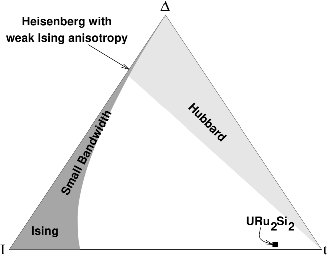
FIG. 3.: Since overall scaling is irrelevant, the space of points $(t,I,\Delta)$ is two-dimensional. Here the points are represented in such a way that $t:I:\Delta=d_{I\Delta}:d_{t\Delta}:d_{tI}$ where $d_{ab}$ is the distance from the point to the line joining $a$ and $b$. The regions we have examined are the shaded ones. (For the purposes of this figure, we interpret $a\ll b$ as $a<b/3$.)

	Energy	States
	$+{\textstyle\frac{1}{4}}\sqrt{I^{2}+4\Delta^{2}}$	$|\!\uparrow\rangle|\!\nearrow\rangle$ ,	$|\!\downarrow\rangle|\!\searrow\rangle$
	$+{\textstyle\frac{1}{2}}\Delta$	$|0\rangle|\!\rightarrow\rangle$ ,	$|\!\uparrow\!\downarrow\rangle|\!\rightarrow\rangle$
	$-{\textstyle\frac{1}{2}}\Delta$	$|0\rangle|\!\leftarrow\rangle$ ,	$|\!\uparrow\!\downarrow\rangle|\!\leftarrow\rangle$
	$-{\textstyle\frac{1}{4}}\sqrt{I^{2}+4\Delta^{2}}$	$|\!\uparrow\rangle|\!\swarrow\rangle$ ,	$|\!\downarrow\rangle|\!\nwarrow\rangle$

FIG. 4.: Spectrum of the independent-site Hamiltonian for $t=0$. Here the first ket represents the conduction electrons: $|\sigma\rangle=c_{\sigma}^{\dagger}|0\rangle$ for $\sigma=\uparrow,\downarrow$; $|\!\uparrow\!\downarrow\rangle=c_{\uparrow}^{\dagger}c_{\downarrow}^{\dagger}|0\rangle$; $|0\rangle$ is the “vacuum”. The second ket represents the state of the localized $f$ electron: $|\!\nearrow\rangle=|\eta_{\theta}\rangle;|\!\searrow\rangle=|\eta_{\pi-\theta}\rangle;|\!\rightarrow\rangle=|\eta_{\pi/2}\rangle;|\!\leftarrow\rangle=|\eta_{-\pi/2}\rangle;|\!\nwarrow\rangle=|\eta_{-\theta}\rangle;|\!\swarrow\rangle=|\eta_{\theta-\pi}\rangle$, and $|\eta_{2\phi}\rangle=(f_{\uparrow}^{\dagger}\cos\phi+f_{\downarrow}^{\dagger}\sin\phi)|0\rangle$ is the state in which the $f$-electron spin lying in the $x$-$z$ plane makes an angle $2\phi$ with the positive $z$-axis measured toward the positive $x$-axis — note that $\langle\eta_{2\phi}|\eta_{2\phi^{\prime}}\rangle=\cos(\phi-\phi^{\prime})$. It is easy to see that here $\theta=\tan^{-1}(2\Delta/I)$ is the tilt produced by the “transverse magnetic field” $\Delta$.

FIG. 5.: Spectrum of the crystal-field Hamiltonian, showing states related to the low-lying singlets by application of the operator $\vec{J}$.

REFERENCES

- [1] C. Broholm, J.K. Kjems, W.J.L. Buyers, P. Matthews, T.T.M. Palstra, A.A. Menovsky, & J.A. Mydosh, Phys. Rev. Lett. 58 (1987) 1467.
- [2] C. Broholm, H. Lin, P.T. Matthews, T.E. Mason, W.J.L. Buyers, M.F. Collins, A.A. Menovsky, J.A. Mydosh, & J.K. Kjems, Phys. Rev. B 43 (1991) 12809.
- [3] A.P. Ramirez, P. Coleman, P. Chandra, E. Brück, A.A. Menovsky, Z. Fisk, & E. Bucher, Phys. Rev. Lett. 68 (1992) 2680.
- [4] V. Barzykin & L.P. Gor’kov, Phys. Rev. Lett. 70 (1993) 2479.
- [5] D.L. Cox, Phys. Rev. Lett. 59 (1987) 1240.
- [6] M.B. Walker, W.J.L. Buyers, Z. Tun, W. Que, A.A. Menovsky, & J.D. Garrett, Phys. Rev. Lett. 71 (1993) 2630; W.J.L. Buyers, Z. Tun, T. Petersen, T.E. Mason, J.-G. Lussier, B.D. Gaulin, & A.A. Menovsky, Physica B 199&200 (1994) 95; M.B. Walker, Z. Tun, W.J.L. Buyers, A.A. Menovsky, & W. Que, Physica B 199&200 (1994) 165.
- [7] T.E. Mason, W.J.L. Buyers, T. Petersen, A.A. Menovsky, & J.D. Garrett, J. Phys.: Cond. Mat. 7 (1995) 5089.
- [8] T.T.M. Palstra, A.A. Menovsky, J. van den Berg, A.J. Dirkmaat, P.H. Kes, G.J. Nieuwenhuys, & J.A. Mydosh, Phys. Rev. Lett. 55 (1985) 2727.
- [9] H. Amitsuka, T. Hidano, T. Honma, H. Mitamura, & T. Sakakibara, Physica B 186-188 (1993) 337.
- [10] T.E. Mason & W.J.L. Buyers, Phys. Rev. B 43 (1991) 11471.
- [11] Note that there is only one centred tetragonal lattice; bct and fct are identical.
- [12] We thank T. Maurice Rice for bringing this to our attention in a private discussion.
- [13] For a review, see I. Affleck, in Fields, Strings and Critical Phenomena, E. Brézin and J. Zinn-Justin, eds., Les Houches XLIX (North-Holland, Amsterdam, 1990) p. 563.
- [14] See, for example, E. Fradkin, Field theories of condensed matter systems, (Redwood City: Addison-Wesley, 1991), p. 32.
- [15] Alternatively, equal-energy surfaces may be used, removing the assumption of sphericity; see I. Affleck, A.W.W. Ludwig, & B.A. Jones, Phys. Rev. B 52 (1995) 9528 (cond-mat/9409100).
- [16] A.J. Leggett, S. Chakravarty, A.T. Dorsey, M.P.A. Fisher, A. Garg, & W. Zwerger, Rev. Mod. Phys. 59 (1987) 1.
- [17] G. Amoretti, A. Blaise, & J. Mulak, J. Mag. Mag. Mat. 42 (1984), 65; G. Amoretti, A. Blaise, R.O.A. Hall, M.J. Mortimer, & R. Troć, J. Mag. Mag. Mat. 53 (1986) 299.