Monte Carlo study of the growth of
$L1_{2}$ ordered domains in fcc $A_{3}B$ binary alloys

Abstract

A Monte Carlo study of the late time growth of $L1_{2}$ ordered domains on a fcc $A_{3}B$ binary alloy is presented. The energy of the alloy has been modeled by a nearest neighbor interaction Ising hamiltonian. The system exhibits a fourfold degenerated ground-state and two kinds of interfaces separating ordered domains: flat and curved antiphase boundaries. Two different dynamics are used in the simulations: the standard atom-atom exchange mechanism and the more realistic vacancy-atom exchange mechanism. The results obtained by both methods are compared. In particular we study the time evolution of the excess energy, the structure factor and the mean distance between walls. In the case of atom-atom exchange mechanism anisotropic growth has been found: two characteristic lengths are needed in order to describe the evolution. Contrarily, with the vacancy-atom exchange mechanism scaling with a single length holds. Results are contrasted with existing experiments in $Cu_{3}Au$ and theories for anisotropic growth.

I Introduction

Kinetics of phase transitions is a problem of great interest not only because of its fundamental importance in non-equilibrium Statistical Physics, but also because its many implications in different areas of Material Science and Technology [1, 2]. The phenomenon is a consequence of the far from-equilibrium initial conditions induced by the sudden change of the imposed thermodynamic parameters on time scales much shorter than the time scales characterizing the process towards the new equilibrium situation. Typically, the system is quenched through its equilibrium ordering temperature. Immediately after the quench, domains of the new phase appear. As time goes on, they grow in size in order to reduce the excess free energy of the walls. This growth shows distinct regimes from early to late times. At late times, in the so called domain growth regime, it is usually assumed that the domain size is much larger than all microscopic lengths in the system. Then, inspired by the situation in equilibrium critical phenomena, it is assumed that the system shows dynamical scaling [3]. This means that at different times the domain structure looks the same when lengths are measured in units of the characteristic length. Furthermore, the average domain size is supposed to increase with time according to a power law with an exponent $x$ characteristic of the universality class to which the system is supposed to belong [4]. If these universality classes really exist, the important point is to identify the distinctive features of a given class. In the simplest case, they are supposed to depend only on whether or not the order parameter is conserved. A typical example for the conserved case is a phase separation process while an order-disorder transition in a binary alloy corresponds to the non-conserved situation. In the first case $x=1/3$ has been predicted while $x=1/2$ is the expected value in the second case [1]. Nevertheless, the concept of universality is not firmly established and is still under discussion. The above classification, just based on the order parameter conservation property, seems to apply only when no disorder is present in the system and the excitations are homogeneously distributed. For instance it is well acknowledged that quenched disorder gives rise to logarithmic growth laws [5], and that excitations localized on the interfaces give rise to exponents greater than 1/2 and 1/3 for the non-conserved and conserved cases respectively [6, 7]. Moreover other parameters like the ground state degeneracy, non-stoichiometry or anisotropic effects could modify the exponents. The exponent $x=1/2$ in non-conserved order parameter systems is theoretically based on a curvature driven interface motion [8]. This is the well known Allen-Cahn law for domain growth. A special curvature driven case leading to an exponent $x=1/4$ has been found for anisotropic systems with a mixture of perfectly flat and curved domain walls [9].

In this paper we will focus on the domain growth problem in a fcc $A_{3}B$ binary alloy undergoing an order-disorder transition from a disordered to a $L1_{2}$ structure. This has been the system most widely used to perform experiments intended to study ordering kinetics in non-conserved order parameter systems [10, 11, 12, 13, 14, 15, 16, 17, 18]. In spite of that, theoretical studies of domain growth in fcc systems are really scarce and, as far as we know, only a recent paper by Lai [19] is specifically devoted to the study of such kind of systems. Concerning computer simulation no data has, to our knowledge, been published. This is a rather surprising fact taking into account that Monte Carlo numerical studies have been of seminal importance in providing much of the quantitative insight into ordering kinetic problems. This is probably due to the inherent complexity of ordering problems in fcc lattices. Actually the ground state is fourfold degenerate and there exist two different kinds of antiphase boundaries: high and low excess energy boundaries. Then, two characteristic lengths may grow following different laws (anisotropic growth) and this can, in some way, question the validity of scaling properties in such a system. In fact, related problems have been considered in $2d$ lattices. For example, the fcc problem has some similarities with the problem of island growth in a system of hydrogen adsorbed on a $(110)$ iron surface with coverage 2/3 [20]. In this case it has been found an exponent smaller than 1/2 which is associated to interface diffusion effects. Also some indications on anisotropic growth are reported in the same reference [20]. Concerning the experimental situation, among a rich literature, it is worth mentioning a pioneer x-ray diffraction work by Cowley [21] devoted to the study of the superstructure peak in $Cu_{3}Au$ single crystals close to equilibrium. Much more recently, a very complete time-resolved x-ray scattering study in a single crystal of $Cu_{3}Au$ [18], has been published. The authors obtain $x=1/2$ with a high degree of accuracy for the growth of the high energetic boundaries and with less degree for the low energetic ones. This leads them to the conclusion that scaling holds in this anisotropic system in agreement with the theoretical predictions by Lai [19].

Our interest in this paper is to present extensive Monte Carlo simulations of the domain growth process performed on a fcc $A_{3}B$ alloy. Since we modelize the system assuming pairwise interactions between nearest neighbor atoms only, the low-energy boundaries have exactly zero excess energy. We expect that this extreme situation emphasize any tendency of the system to show anisotropic growth effects. In addition we will perform simulations in systems either with and without vacancies (in this last case only vacancy-atom exchanges will be allowed) in order to investigate the effect of the vacancy mechanism in the kinetics of ordering in fcc lattices. This mechanism has, recently, been shown to play a very important role in bcc lattices [22].

The paper is organized as follows. In the next section we introduce the model and describe some of the features of the ground state and the domain walls. In section III we explain the details of the Monte Carlo simulations and define the different magnitudes used to describe the ordering process. The results are sequentially presented in section IV and discussed in section V. Finally, in section VI, we give a summary of the main conclusions.

II Model and ground state

The binary alloy is modeled by a set of $N_{A}$ $A$-atoms, $N_{B}$ $B$-atoms and $N_{V}$ vacancies on a “perfect” fcc lattice with lattice spacing $a$, linear size $a\,L$ and periodic boundary conditions. The number of lattice sites is $N=4L^{3}=N_{A}+N_{B}+N_{V}$. Assuming nearest neighbors (n.n.) interactions only, a general ABV model hamiltonian [23] can be rewritten as a Blume-Emery-Griffiths [24] one, as explained in Refs. [22, 25]:

$${\cal H}=J\sum_{\left\langle i,j\right\rangle}^{\rm n.n.}S_{i}S_{j}+K\sum_{\left\langle i,j\right\rangle}^{\rm n.n.}S_{i}^{2}S_{j}^{2}+L\sum_{\left\langle i,j\right\rangle}^{\rm n.n.}\left(S_{i}^{2}S_{j}+S_{i}S_{j}^{2}\right)+{\cal H}_{0},$$ (1)

where the sums extend over all n.n. pairs and $i$ and $j$ are generic indexes sweeping all the lattice ($i,j=1,\dots N$). The spin variables $S_{i}$ can take three values: $+1$, $-1$ and $0$ when the $i$-th position of the lattice is occupied by an $A$-atom, a $B$-atom or a vacancy respectively. The parameters $J$, $K$ and $L$ are coupling parameters and ${\cal H}_{0}$ is a function of the concentration. In the case of low vacancy concentrations ($N_{V}\ll N_{A},N_{B}$) this hamiltonian can be approximated by a spin-1 Ising model:

$${\cal H}=J\sum_{\left\langle i,j\right\rangle}^{\rm n.n.}S_{i}S_{j},$$ (2)

except for an irrelevant additive constant. This is the hamiltonian that we have used in the present simulations.

We have focused on the case $N_{A}\simeq 3N_{B}\gg N_{V}$ in order to simulate an $A_{3}B$ alloy like $Cu_{3}Au$, $Ni_{3}Mn$ or $Ni_{3}Fe$, with little concentration of vacancies. It is well known that for $J>0$ and no vacancies ($N_{V}=0$) this system presents a discontinuous order-disorder phase transition when temperature is increased [26, 27, 28]. The ordered phase is the so called $L1_{2}$ structure. The fcc lattice can be regarded as four inter-penetrated simple cubic sublattices (named $\alpha$, $\beta$, $\gamma$ and $\delta$ in Fig. 1); the perfect $L1_{2}$ order consists in three sublattices full of $A$-atoms and the other one full of $B$-atoms so that it is fourfold degenerated. The four equivalent kinds of ordered domains will be called $\alpha$-, $\beta$-, $\gamma$- and $\delta$-domains according to the sublattice which contains the minority specie $B$. The order is described by means of the three following long-range order parameters [19]:

$$\Psi_{1} = \frac{2}{N}\sum_{ijk\;\xi\eta\zeta}S_{ijk\;\xi\eta\zeta}(-1)^{\xi}$$ (3)

$$\Psi_{2} = \frac{2}{N}\sum_{ijk\;\xi\eta\zeta}S_{ijk\;\xi\eta\zeta}(-1)^{\eta}$$ (4)

$$\Psi_{3} = \frac{2}{N}\sum_{ijk\;\xi\eta\zeta}S_{ijk\;\xi\eta\zeta}(-1)^{\zeta}$$ (5)

where $S_{ijk\;\xi\eta\zeta}$ is the spin-variable at position $\vec{r}_{ijk\;\xi\eta\zeta}=a(i+\xi/2,j+\eta/2,k+\zeta/2)$, and $i,j,k$ range from $1$ to $L$ and the vector $(\xi,\eta,\zeta)$ take values $(0,0,0)$, $(0,1,1)$, $(1,0,1)$ and $(1,1,0)$ pointing to the position of the four sublattices $\alpha$, $\beta$, $\gamma$ and $\delta$ respectively.

After a quench through the equilibrium transition temperature $T_{0}$, the four possible degenerated domains appear and compete during the domain growth regime. It is well known [11, 18, 19, 29, 30] that two kinds of antiphase domain boundaries (APDB) exist (see Fig. 2):

1. The first type (named type-1 or “half diagonal glide” walls) of APDB corresponds to a displacement vector contained in the plane of the APDB. This kind of boundaries maintain the same number of $A-B$ n.n. bonds as in the ordered bulk. Hence, in our model with n.n. interactions only, such boundaries do not suppose any excess of energy. It is also interesting to remark that they can only appear in specific directions depending on the two adjacent domains: for instance they can appear perpendicular to direction [100] between $\alpha$- and $\beta$-domains and between $\gamma$- and $\delta$-domains. Table I shows the directions of the type-1 walls for all the possible neighboring domains. Moreover, it is possible to build up a structure combining the different kinds of ordered domains with only type-1 walls, i.e. without excess of energy. At low temperatures, such structure would not evolve in time.

2. The second type of APDB (type-2 walls) corresponds to a displacement vector not contained in the boundary plane. Since it does not maintain the same number of $A-B$ n.n. bonds as in the bulk, it contributes with a positive excess of energy. It should also be mentioned that these boundaries contain a local excess of particles (either $A$ or $B$) and they are wider than the type-1 walls.

III Monte Carlo simulation details

A Dynamics

We have performed two kind of simulation studies:

1. The first kind includes the simulations of the ordering processes without vacancies ($N_{V}=0$), which have been performed using the standard Kawasaki dynamics proposing exchanges between n.n. atoms.

2. The second kind includes the simulations with vacancies. In this case we have used a restricted Kawasaki dynamics proposing n.n. vacancy-atom exchanges (vacancy jumps) only. This dynamics is more realistic in studying ordering kinetics in binary alloys. The concentration of vacancies has been taken the same in all the simulations ($c_{V}\equiv N_{V}/N\simeq 3.1\,10^{-5}$).

The concentration of particles is preserved by both dynamics while the order parameters are not. In both cases we have accepted or refused the proposed exchange using the usual Metropolis acceptance probability:

$$p(\Delta{\cal H})=\left\{\begin{array}[]{ll}1&{\rm if}\;\Delta{\cal H}\leq 0\\ exp\left\{-\frac{\Delta{\cal H}}{k_{B}T}\right\}&{\rm if}\;\Delta{\cal H}>0\end{array}\right.,$$ (6)

where $\Delta{\cal H}$ is the energy change associated to the proposed exchange. We define the unit of time, the Monte Carlo step ($mcs$), as the trial of $N$ exchanges (either atom-atom or vacancy-atom exchanges). In all the cases we have started the simulations from a completely disordered state, as would correspond to a system at $T=\infty$. The system is then suddenly quenched into a final temperature $T_{q}$ below the transition temperature $T_{0}$. To prepare the disordered states we fill up the system with $A$-atoms and randomly replace $N/4$ of these $A$-atoms by $B$ ones; when it is necessary, we also choose at random $N_{V}$ lattice sites to place the vacancies.

B Measurements

Our main interest is the description of the time evolution of the ordered domains. Usually, the domain size is measured as the inverse of the excess energy, which is proportional to the amount of interface [31]. Nevertheless, in our case, there are two coexisting types of interfaces and only the amount of type-2 walls might be related to the excess energy as has been discussed in section II. Consequently for fcc lattices with $L1_{2}$ order it is convenient to simultaneously measure both the excess energy and the structure factor. These two quantities are defined as follows:

1. Excess energy per site:

   $$\Delta E(t)\equiv\frac{1}{N}\left[{\cal H}(t)-{\cal H}(t\rightarrow\infty)\right],$$ (7)

   where ${\cal H}(t\rightarrow\infty)$ is the equilibrium energy at the quenching temperature $T_{q}$.

2. Structure factor:

   $$S(\vec{k},t)\equiv\left|\frac{1}{N}\sum_{ijk\;\xi\eta\zeta}S_{ijk\;\xi\eta\zeta}\exp\left\{{\bf i}\frac{2\pi}{a}\vec{k}\cdot\vec{r}_{ijk\;\xi\eta\zeta}\right\}\right|^{2},$$ (8)

   where the sum extends over the whole lattice, ${\bf i}$ is the imaginary constant and $\vec{k}$ is the dimensionless reciprocal vector. The discreteness of the real space makes the structure factor to be invariant under the $\langle 200\rangle$ translations in the reciprocal space. The periodic boundary conditions imply that the reciprocal space is discrete on a cubic lattice on the $\vec{k}$-space with lattice spacing ${\displaystyle\frac{1}{L}}$. Figure 3 shows the reciprocal space with the position of the fundamental and the superstructure peaks.

C Domains and superstructure peak

The temporal evolution of the domain structure is illustrated in Fig. 4(a,b,c). Three snapshots, at selected times, corresponding to a section parallel to the (100) planes are presented. The four possible ordered regions are indicated with different colors. Flat (type-1) and curved (type-2) interfaces can be observed. The mean distance between such walls is related to the shape of the superstructure peaks of the structure factor. Discrepancies in the shape of these peaks have been reported in the literature. Old x-ray measurements by Cowley [21] suggested that the peaks are square shaped. More recently it has been insinuated that the peaks are disk shaped [18]. Our simulations give square (or even star-like) shaped peaks as it can be seen in the temporal sequence presented in Fig. 4(d,e,f). Such anisotropy in the peak shape does not necessarily imply that the ordered domains are needle shaped, but arises from the correlation between the ordered domains. For instance the superstructure peak at (100) position accounts for the long range order parameter $\Psi_{1}$. This order parameter does not discriminates between $\alpha$- and $\beta$-domains (both having $\Psi_{1}=-1$) nor between $\gamma$- and $\delta$-domains (both having $\Psi_{1}=1$). The tendency of the domains to locate in such a way that the interfaces does not have extra energy favors the formation of $\alpha$-$\beta$ and $\gamma$-$\delta$ boundaries (type-1) perpendicular to the [100] direction. Therefore the regions with a high value of the order parameter $\Psi_{1}$ are anisotropic, producing the anisotropy of the $(100)$ peak. The same happens for the other peaks at $(010)$ and $(001)$.

The inverse of the amplitudes of the superstructure peak along both, the radial ($\sigma_{r}$) and the transverse ($\sigma_{t}$) directions, are related to the mean distance between type-2 and type-1 walls respectively. The measurement of $\sigma_{r}$ has been done by analyzing the profile of:

$$S_{r}(q,t) = \frac{1}{3}\left[S\left((1,0,0)-\frac{1}{L}(q,0,0),t\right)+\right.S\left((0,1,0)-\frac{1}{L}(0,q,0),t\right)+$$ (10)

$$\left.S\left((0,0,1)-\frac{1}{L}(0,0,q),t\right)\right],$$

where $q=0,1,\dots,L$ is the distance from the superstructure peak (in units of ${\displaystyle\frac{1}{L}}$). Following the notation in Ref. [18], we will refer to this profile as the radial scan of the structure factor. It corresponds to the average on the three thick continuous lines of Fig. 3. The measurement of $\sigma_{t}$ has been done by analyzing the profile of:

$$S_{t}(q,t) = \frac{1}{6}\left[S\left((1,0,0)+\frac{1}{L}(0,0,q),t\right)+S\left((1,0,1)-\frac{1}{L}(0,0,q),t\right)+\right.$$ (13)

$$S\left((0,1,0)+\frac{1}{L}(q,0,0),t\right)+S\left((1,1,0)-\frac{1}{L}(q,0,0),t\right)+$$

$$\left.S\left((0,0,1)+\frac{1}{L}(0,q,0),t\right)+S\left((0,1,1)-\frac{1}{L}(0,q,0),t\right)\right],$$

where $q=0,1,\dots,L/2$. We will refer to it as transverse scan of the structure factor. It corresponds to the average on the two symmetric parts of the three thick dashed lines of Fig. 3. It can be easily shown that due to the symmetries of the structure factor the average over the continuous (dashed) thick lines is equal to the average over all the continuous (dashed) lines of the Fig. 3. In addition, at every time both profiles have been averaged over a certain number of independent runs (about 25 for $L=64$ and 40 for the other system sizes). This last average is indicated by means of angular brackets ($\langle\cdots\rangle$). The finite size effects have been studied by simulating systems of linear sizes $L=$ 20, 28, 36 and 64 ($N=$ 32000, 87808, 186624 and 1048576 sites respectively). We have also studied the effect of the quenching temperature performing simulations at $T_{q}=1.0J/k_{B}$ ($T_{q}/T_{0}\simeq 0.55$) and $T_{q}=1.5J/k_{B}$ ($T_{q}/T_{0}\simeq 0.83$).

D Fitting procedure for $\sigma_{r}$ and $\sigma_{t}$

We have measured $\sigma_{r}$ and $\sigma_{t}$ using the two following methods.

1. The first method is based on the evaluation of the second moment of the scan:

   $$\sigma^{2}(t)\equiv\frac{\displaystyle\sum_{q=0}^{q_{max}}q^{2}\langle S(q,t)\rangle}{\displaystyle\sum_{q=0}^{q_{max}}\langle S(q,t)\rangle}$$ (14)

   where $S$ represents either $S_{r}$ or $S_{t}$, and $q_{max}$ is the first $q$-value for which $\langle S(q,t)\rangle$ is lower than a background threshold. The value of this background has been taken double of the mean value of the structure factor of a completely disordered system (excluding the fundamental peak).

2. The second method is based on the fitting of a lorentzian function to the data of the corresponding scan. In order to account for the large-$q$ tail of the structure factor we have fitted $\log\langle S(q,t)\rangle$ to the three-parameters ($a$, $\sigma$, $B$) function:

   $$\log\langle S(q,t)\rangle\simeq\log\left\{\frac{a}{\left[1+{\displaystyle\left(\frac{q}{\sigma(t)}\right)^{2}}\right]^{\alpha}}+B\right\},$$ (15)

   where $\sigma$ is the estimation of the width, $B$ is the background, $a$ is the fitted intensity and $\alpha$ is an exponent (not fitted) that we discuss in the next paragraph.

We have analyzed the validity of both methods for the two scans of the structure factor. The first method turns out to be adequate only for the radial scans. This is because the large-$q$ tail of the transverse scan decays very slowly and, therefore, $\sigma_{t}$ is strongly affected by the choice of $q_{max}$. The second method can be used for both scans. Moreover, both methods render equivalent results for radial scans. Therefore we will estimate $\sigma_{r}$ using method 1 and $\sigma_{t}$ using method 2. Concerning the exponent $\alpha$ we have tried $\alpha=1,2$ and $3/2$ for both scans. In general the best fits to the radial scan have been obtained with $\alpha=3/2$, while for the transverse scans $\alpha=1$ gives the best results.

E Scaling

We have tested the existence of dynamical scaling in both the radial and the transverse directions by plotting the corresponding scaling function $\tilde{S}(\tilde{q})$ defined from the following expression:

$$\langle S(q,t)\rangle=\frac{1}{\sigma(t)^{d}}\tilde{S}(\tilde{q}),$$ (16)

where $\displaystyle\tilde{q}=\frac{q}{\sigma(t)}$ is the scaling variable and $d$ is the space dimensionality. Scaling has been tested by checking the overlap of the data corresponding to different times and also to different system sizes. Theoretical predictions for the scaling function $\tilde{S}(\tilde{q})$ exist [3, 19], specially concerning the behaviour for large values of $q$.

IV Results

For the sake of clarity the results are presented in the following order: first, the results corresponding to equilibrium simulations (subsection A); second, those concerning the evolution of the system using the atom-atom exchange mechanism (subsection B); and third, the results obtained by means of the vacancy-atom exchange mechanism (subsection C). The results in subsections B and C are always given at quenching temperatures $T_{q}=1.0J/k_{B}$ and $T_{q}=1.5J/k_{B}$. The structure factor profiles are only presented for $L=64$ although data corresponding to smaller $L$ have also been analyzed.

A Equilibrium

Starting from perfectly ordered systems with $L=20$, we have step-by-step heated them from $T=0.5J/k_{B}$ to $T=3.0J/k_{B}$ and cooled them again down to $T=0.5J/k_{B}$. At each temperature we have let the system to reach equilibrium (after $\sim 12\;10^{3}mcs$) and have obtained the equilibrium energy ${\cal H}(t\rightarrow\infty)$ and the mean long range order parameter defined as:

$$\Psi\equiv\frac{|\Psi_{1}|+|\Psi_{2}|+|\Psi_{3}|}{3}.$$ (17)

The temporal average of this order parameter is presented in Fig. 5 as a function of temperature. No differences can be observed between the cases corresponding to $N_{V}=0$ (with the atom-atom exchange mechanism) and $N_{V}=1$ (with the vacancy-atom exchange mechanism). We have found that the transition is first order and that the heating-cooling cycle shows hysteresis. The transition temperature has been estimated to be $T_{0}=1.81\pm 0.03J/k_{B}$ compatible with the Monte Carlo results given in Ref. [28].

B Atom-atom exchange mechanism

Figures 6(a) and 6(b) show the profiles, at different times, of the radial scan of the structure factor for the two studied quenching temperatures. The corresponding structure factors, scaled according to eq. (16), are shown in Fig. 7. In general, the overlap of the different curves is quite good. It has been checked that data corresponding to different system sizes also fall on the same curve. Nevertheless, deviations from this scaling can be well appreciated at $q=0$ in Fig. 7(a) ($T_{q}=1.0J/k_{B}$). We will come back to this point in the discussion. The continuous lines show fits of lorentzian functions [eq. (15)] with $\alpha=3/2$ and $\sigma=1$ which corroborates the validity of such kind of fitting function for all the individual profiles. The insets in Fig. 7(a) and Fig. 7(b) display log-log plots of the scaled radial scans: for large $\tilde{q}$-values $\tilde{S}_{r}(\tilde{q})$ decays as $\tilde{q}^{-3}$, as indicated by a continuous line.

Figures 8(a) and 8(b) show log-log plots of the time evolution of $\langle\Delta E(t)\rangle$ and $\sigma_{r}(t)$ for different system sizes and the two studied quenching temperatures. Solid straight lines are the following fitted power-laws:

$$\langle\Delta E(t)\rangle \sim t^{-x}$$ (18)

$$\sigma_{r}(t) \sim t^{-y}.$$ (19)

The behaviour of the growth-exponents $x$ and $y$ for the two quenching temperatures are presented in Fig. 9 in front of $1/L$. The corresponding numerical values are listed in Table II. The estimations of the two growth exponents, $x$ and $y$, are coincident within the errors bars. A general tendency of the exponent to increase when temperature is increased and to decrease when increasing the system size is observed. Extrapolation to $L\rightarrow\infty$, following the method explained in section V, renders $x\simeq y\simeq 0.40$ for $T_{q}=1.0J/k_{B}$ and $x\simeq y\simeq 0.44$ for $T_{q}=1.5J/k_{B}$

Figure 10 shows linear-log plots of the transverse scan of the structure factor for the two studied quenching temperatures, at different times. The corresponding scaled transverse scans are shown in Fig. 11. The overlap of the curves is rather satisfactory, however it is not as broaden in time as for the radial scan case. Note that in Fig. 11(b) lack of scaling at $q=0$ is clearly evident. As for the radial scan case, we have also verified the overlap of the data corresponding to systems with different sizes. The continuous lines show fits of lorentzian functions [eq. (15)] with $\alpha=1$ and $\sigma=1$. The insets display log-log plots of these scaled transverse scans: in this case $\tilde{S}_{t}(\tilde{q})$ decays as $\tilde{q}^{-2}$ for large $\tilde{q}$, as indicated by the continuous line.

Log-log plots of the time evolution of $\sigma_{t}(t)$ for different system sizes and the two studied quenching temperatures are presented in Fig. 12. Solid straight lines correspond to the fitted power-law:

$$\sigma_{t}(t)\sim t^{-z}$$ (20)

The values of the growth exponents are listed in Table II and plotted in front of $1/L$ in Fig. 9. In this case, the extrapolations to $L\rightarrow\infty$ render $z\simeq 0.26$ for $T_{q}=1.0J/k_{B}$ and $z\simeq 0.47$ for $T_{q}=1.5J/k_{B}$. The time evolution of the order parameter, i.e. the structure factor at $q=0$ ($\langle{\displaystyle S_{r}(q=0,t)\rangle=\langle S_{t}(q=0,t)\rangle=\left\langle\frac{\Psi_{1}^{2}+\Psi_{2}^{2}+\Psi_{3}^{2}}{3}\right\rangle}$), is shown in Fig. 13.

C Vacancy-atom exchange mechanism

The profiles of the radial scans of the structure factor can be seen in Fig. 14. The same data scaled according eq. (16) are shown in Fig. 15. The overlap of the different curves corroborates the scaling hypothesis. It is worth noting that scaling holds even at $q=0$, contrarily to the case of atom-atom exchange mechanism at low quenching temperature. Scaling of data corresponding to different system sizes has also been checked. The continuous lines show fits of lorentzian functions [eq. (15)] with $\alpha=3/2$ and $\sigma=1$. The log-log plots shown in the insets of Fig. 15 reveal that, for large $\tilde{q}$, $\tilde{S}_{r}(\tilde{q})$ decays as $\tilde{q}^{-3}$, as indicated by the continuous line.

Figure 16 shows a log-log plot of the time evolution of $\sigma_{r}(t)$, $\langle\Delta E(t)\rangle$ and the best fits of the power laws defined by eq. (19). The resulting $x$ and $y$ exponents, are listed in Table III, and plotted in front of $1/L$ in Fig. 17. Extrapolations to $L\rightarrow\infty$ render $x\simeq y\simeq 0.36$ for $T_{q}=1.0J/k_{B}$ and $x\simeq y\simeq 0.44$ for $T_{q}=1.5J/k_{B}$.

The profiles of the transverse scan of the structure factor are plotted in Fig. 18. The same data is presented in scaled form in Fig. 19. Notice that the scaling is again satisfied at $q=0$. Scaling also holds for data corresponding to different system sizes. The continuous lines show fits of lorentzian functions [eq. (15)] with $\alpha=1$ and $\sigma=1$. The behavior of the tail is $\tilde{S}_{t}(\tilde{q})\propto\tilde{q}^{-2}$, as we obtained for the atom-atom exchange case.

The time evolution of $\sigma_{t}(t)$ can be seen in Fig. 20 and the fitted exponents according to eq. (20) are plotted in Fig. 17 and listed in Table III. The extrapolations to $L\rightarrow\infty$ render $z\simeq 0.34$ for $T_{q}=1.0J/k_{B}$ and $z\simeq 0.44$ for $T_{q}=1.5J/k_{B}$. Finally, the time evolution of the order parameter is shown in Fig. 21.

V Discussion

The analysis of the growth exponents for finite $L$ reveals that, independently of the exchange mechanism and temperature, the exponents $x$ and $y$ corresponding to $\langle\Delta E(t)\rangle$ and $\sigma_{r}(t)$ respectively, coincide within errors bars: the obtained numerical value is, at low temperature, lower than the Allen-Cahn growth exponent $1/2$; nevertheless it raises towards such value when approaching the order-disorder transition temperature. The value $y=1/2$ has been obtained experimentally [18] with high accuracy at quenching temperatures $T_{q}$ ranging from $0.96T_{0}$ to $0.99T_{0}$ (our greatest simulated value is $T_{q}=0.83T_{0}$). Concerning the exponent $z$, characterizing the growth of $\sigma_{t}$, we obtain $z\simeq x\simeq y$ for the case of vacancy-atom exchange mechanism and $z<x\simeq y$ for the case of atom-atom exchange mechanism. In the later case, the difference becomes more important with decreasing temperature. We expect that, even in this case, $z$ will reach the value $1/2$ when $T_{q}$ approaches $T_{0}$. Experimentally, no clear differences have been observed between $y$ and $z$. This could be due either to the fact that the relevant physical mechanism for the growth is the vacancy-atom exchange, or that the experiments are performed at temperatures too close to $T_{0}$. Nevertheless our simulation results, at low temperatures, suggest that the evolution of $\sigma_{t}$ cannot be described by the standard Allen-Cahn growth law. Additional physical considerations are needed in order to describe the evolution of such flat interfaces in the case of atom-atom exchange mechanism.

From the values of the exponents corresponding to different system sizes we have performed a finite size analysis following the method proposed in Ref. [22]. This analysis assumes a first order correction to the growth law according to:

$$R(t)\sim t^{n}\left(1-\frac{b}{t}\right),$$ (21)

where $n$ stands for any of the growth exponents $x$, $y$ or $z$. This implies that the finite size dependence of the exponent $n_{L}$ follows:

$$n_{L}=n_{\infty}+bL^{-1/n_{\infty}}.$$ (22)

Fits of this equation to the obtained exponents are plotted (solid lines) in Figs. 9 and 17. The resulting values of $n_{\infty}$ are shown in Tables II and III. These extrapolated values confirm the points discussed in the previous paragraph. The values of the first order correction coefficient $b$ are shown in Table IV. For the case of atom-atom exchange mechanism the sign of the coefficients $b$ corresponding to the exponents $z$ are negative reinforcing the suggestion that the standard Allen-Cahn growth law does not hold in this case. It is also interesting to remark that, in general, the coefficient $b$ is greater for the vacancy-atom exchange mechanism than for the atom-atom exchange one. This confirms that in the former case the exponents exhibit a greater dependence with finite size. This is in agreement with previous results reported for 2-d square lattices [25].

Concerning the scaling of the structure factor, it is worth noting that it holds in a broad range of time for all the studied cases indicating that the domain growth regime, in which the evolution of the system is governed by two characteristic lengths proportional, respectively, to $\sigma_{r}^{-1}$ and $\sigma_{t}^{-1}$, is clearly reached in our simulations. Whether or not both lengths obey the same growth law can be detected by the scaling of the structure factor at $q=0$. At this $q$-position, scaling holds only if $\sigma_{r}(t)\propto\sigma_{t}(t)$. For the case of vacancy-atom exchange mechanism scaling at $q=0$ is definitively satisfied, indicating that a single growth law governs the evolution of the system consistently with an unique value of the growth exponents ($x\simeq y\simeq z$). Contrarily, for the case of atom-atom exchange mechanism, a lack of scaling at $q=0$ can be clearly seen in Figs. 7 and 11 (compare with Figs. 15 and 19 at $q=0$). This indicates that the two lengths are needed to characterize the evolution of the system in this case.

The time evolution of the order parameter [$\langle S(q=0)\rangle$] shown in Figs. 13 and 21 is in qualitative good agreement with the experimental results for $Cu_{3}Au$ (see Fig. 18 in Ref. [18]). Even the existence of a possible delay time due to an incubation period for nucleation, that has been found experimentally, can be observed as an inflexion point in our curves. In our model the disordered phase is metastable down to zero temperature due to frustration effects [28]. Therefore the evolution, in our simulations, initiates via nucleation, as expected [32, 33] for $Cu_{3}Au$ in the experimentally studied temperature range [18]. Also in agreement with experiments, the delay time increases with increasing $T_{q}$. The experimentalists [18] suggest an explanation for this delay based on the influence of the elastic energy in the nucleation process. Despite not containing elastic effects our model reproduces such results, indicating that a full explanation cannot rely only on elasticity arguments. Moreover, comparing Figs. 13(b) and 21(b) it seems that the delay is more important in the case of the vacancy mechanism. This problem will be studied in a future work.

The behaviour of the tail of the structure factor along the radial and the transverse directions is markedly different. This can be clearly seen by comparing the insets of Figs. 7 and 15 corresponding to the radial scans and those in Figs. 11 and 19 corresponding to the transverse scans. For such anisotropic peaks, the Porod’s Law [34], $\langle S(q)\rangle\sim q^{-(d+1)}$, ($d+1=4$ in our case) is not expected to be satisfied. Independently of the dynamical exchange mechanism we have found that for large values of $q$, $\langle S_{r}(q)\rangle\sim q^{-3}$ and $\langle S_{t}(q)\rangle\sim q^{-2}$. This is in agreement with the fact that the best lorentzian fits are obtained for $\alpha=3/2$ and $\alpha=1$ for radial and transverse scans respectively, as explained in section III. We have also studied the dependence of $\langle S(q)\rangle$ for large $q$ along the diagonal direction [$\vec{k}=(1,1,0)+\frac{1}{L}(q,q,0)$]. Figure 22 compares the decay along this direction with the transverse and radial ones. For the diagonal direction, results are consistent with a $q^{-3}$ decay. This reveals the singular character of the behaviour along the transverse direction. It is interesting to remark that the present simulation results are not in agreement with the theory for ordering dynamics in $Cu_{3}Au$ proposed by Lai [19]. In that theory it is found that the Porod’s Law is satisfied for both radial and transverse scans. This important difference between Lai’s theory and the present simulation probably arises from the fact that in our model type-1 walls have zero excess energy.

Concerning the previous studies of the order-disorder dynamics by means of the vacancy-atom exchange mechanism some important differences must be pointed out. Firstly, for two dimensional square [35] and bcc lattices [22] vacancies are known to accelerate the growth leading, at low temperatures, to exponents $x>1/2$. This is due to the fact that the vacancy prefers to move along the interfaces, increasing the number of accepted exchanges. Such acceleration only appears if the vacancy is allowed to jump to next-nearest neighbor (n.n.n.) positions. Such jumps prevent the vacancy to be trapped in the ordered regions. When only jumps to n.n. positions are permitted, the growth law becomes logarithmic. Although in the present simulations on fcc lattices we only allow vacancy jumps to n.n. positions, trapping does not appear since for such fcc lattices the ordered regions can be crossed without energy barriers. We have tested, by performing a number of simulations allowing the vacancy to jump to n.n.n. positions, that the growth exponents do not change significantly. Secondly, for the present simulations the acceleration of the domain growth process compared to the atom-atom exchange mechanism does not appear. This is due to the fact that the tendency for the vacancy to sit on the interfaces is quite low in this case: some of the interfaces are non energetic and, among the energetic ones, only those with an excess of the majoritary specie represent an energy gain for the vacancy compared to the bulk. Consequently the vacancy path in this case is much more homogeneous (close to a random walk) than for the case of a bcc lattice (close to a self-avoiding walk) [22].

Finally, there is still a very important question to be answered: Why, in the case of vacancy-atom exchange mechanism, the growth can be described by a single length whereas two different lengths are needed in the atom-atom exchange mechanism case? Actually, for the case of atom-atom exchange mechanism the need of two characteristic lengths is expected, as has been found in several studies of anisotropic growth. For instance, in a two-dimensional model for a martensitic transition [9], the existence of two relevant lengths arises as a consequence of the coexistence of flat and curved interfaces, that can only evolve in a hierarchical way: the curved interfaces have to wait for the planar interfaces to disappear before they can decrease in length. It is worth mentioning that in such model the anisotropy is explicitly introduced in the hamiltonian, while in the present case anisotropy appears due to the topology of the fcc lattice. It is found, in agreement with our result using the atom-atom (at low $T_{q}$) exchange mechanism, that the mean distance between planar interfaces grows as $t^{1/4}$ and that the mean distance between curved interfaces grows as $t^{1/2}$. Also, in a model for island growth [20], the anisotropic growth appears as a consequence of the coexistence of two kinds of interfaces. The surprising result is that the vacancy-atom exchange mechanism destroys the expected anisotropic growth. We cannot provide a definitive explanation for this question at present; nevertheless, we believe that the sequentiality of the vacancy path modifies the hierarchical motion of the planar and curved interfaces existing in the system.

VI Summary and conclusions

In this paper extensive Monte Carlo simulations of $L1_{2}$ ordering kinetics on a fcc $A_{3}B$ binary alloy are presented. We have focused on the study of the evolution of the superstructure peak and the excess energy. We have followed the growth up to $10^{4}\;mcs$ in systems with linear size ranging from $L=20$ to $L=64$. Two different dynamics have been used: first the standard Kawasaki atom-atom exchange mechanism and second, the more realistic vacancy-atom exchange mechanism. In this last case a very small concentration of vacancies is introduced in the system. Finite size scaling techniques have been used in order to extrapolate to $L\rightarrow\infty$ the growth exponents evaluated at finite $L$. We have obtained that finite-size effects are more important in the case of the vacancy-atom exchange mechanism. For the atom-atom exchange mechanism we have found evidences of anisotropic growth: the width of the superstructure peak in the transverse direction evolves according to $\sigma_{t}\sim t^{-z}$ with $z$ smaller than the exponent $y$ characterizing the evolution of the width in the radial direction $\sigma_{r}\sim t^{-y}$. Such anisotropy arises from the hierarchical interface motion of the two different domain walls. As proposed in a recent theory [9], this leads to $y=1/2$ and $z=1/4$ in rather good agreement with our experimental results. Contrarily, for the vacancy-atom mechanism, the two relevant lengths $\sigma_{t}^{-1}$ and $\sigma_{r}^{-1}$ evolve following the same power law. The disappearance of the anisotropic growth with the vacancy-atom exchange mechanism may arise from the fact that the sequentiality of the vacancy path destroys the hierarchical evolution of the two different interfaces existing in the system.

The effect of the temperature has also been studied. For both mechanism the exponents $y$ and $z$ tend to 1/2 when the transition temperature is approached from below. To our knowledge, all the experiments have been performed at $T_{q}\sim T_{0}$, so that no conclusive results about the relevant ordering mechanisms can be deduced. The results in this paper suggest that more experimental studies of the ordering dynamics, specially at low temperatures, are desirable in order to clarify the existence of such anisotropic growth and which is the relevant mechanism for ordering. Synchrotron radiation facilities seem to be very promising for the obtention of the needful structure factor maps in the late time regime.

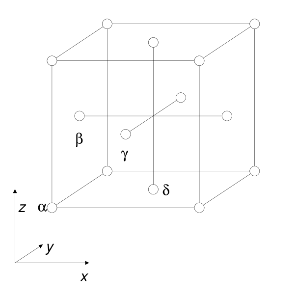
FIG. 1.: The four sublattices $\alpha$, $\beta$, $\gamma$ and $\delta$ in to which the fcc lattice can be divided.

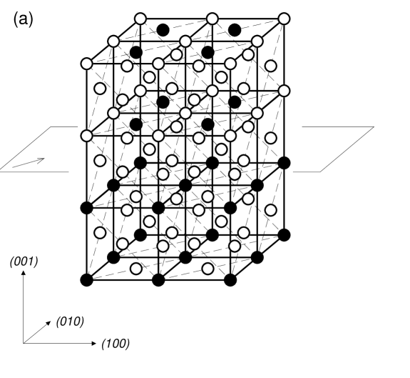
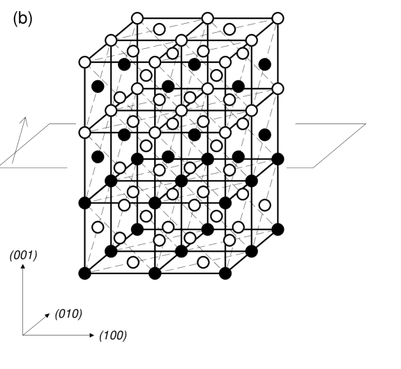
FIG. 2.: Schematic picture of the two kinds of APDB explained in the text, (a) type-1 wall conserving the energy of the system, (b) type-2 wall with an excess of unsatisfied bonds. The arrows indicate one of the four equivalents directions in which the displacement can be made.

FIG. 3.: Reciprocal $\vec{k}$-space showing the fundamental (filled circles) and the superstructure (squares) peaks. The average of the structure factor on the thick solid lines is $S_{r}(q,t)$ and the average on the thick dashed lines is $S_{t}(q,t)$.

FIG. 4.: Snapshots of the system evolution in real space [(a), (b) and (c)] and in reciprocal space [(d), (e) and (f)]. The real space pictures, corresponding to a section perpendicular to (100) direction, show in four different colors the structure of ordered domains. The reciprocal space plots show the structure factor maps in the plane (100) with color scale increasing logarithmically from violet to yellow. Data corresponds to a simulation using the atom-atom exchange mechanism at $T_{q}=1.0$, system size $L=64$, and times $t=18\;mcs$ [(a) and (d)], $t=198\;mcs$ [(b) and (e)] and $t=1998\;mcs$ [(c) and (f)].

FIG. 5.: Equilibrium order parameter as a function of temperature for $L=20$ with (a) $N_{V}=0$ (atom-atom exchanges) and (b) $N_{V}=1$ (vacancy-atom exchanges). The insets show in detail the hysteresis due to the discontinuous character of the transition. From both figures it can be concluded that $k_{B}T_{c}/J=1.81\pm 0.03$. Squares correspond to a heating process while circles to a cooling one.

FIG. 6.: Linear-log plot of the averaged radial scan of the structure factor at different times and quenching temperatures $T_{q}=1.0J/k_{B}$ (a) and $T_{q}=1.5J/k_{B}$ (b). Both graphs correspond to systems of linear size $L=64$ for the atom-atom exchange mechanism.

FIG. 7.: Linear-log and log-log (insets) plots of the scaled radial scan of the structure factor at different times and quenching temperatures $T_{q}=1.0J/k_{B}$ (a) and $T_{q}=1.5J/k_{B}$ (b). Data corresponds to systems of linear size $L=64$ for the atom-atom exchange mechanism. The solid thick line corresponds to a fit of expression (3.7) with $\alpha=1.5$ and $\sigma=1$. The dashed lines in the insets show the Porod’s law $\tilde{S}_{r}(\tilde{q})\sim\tilde{q}^{-4}$, while solid lines show the slope of $\tilde{q}^{-3}$.

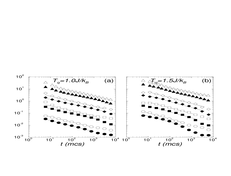
FIG. 8.: Time evolution, in the case of atom-atom exchange mechanism, of $\langle\Delta E(t)\rangle$ (filled symbols) and of $\sigma_{r}(t)$ (open symbols), for $T_{q}=1.0J/k_{B}$ (a) and $T_{q}=1.5J/k_{B}$ (b) for systems of $L=20$ (circles), $L=28$ (squares), $L=36$ (diamonds) and $L=64$ (triangles). The solid lines are the best power-law fits. Data corresponding to different sizes have been vertically shifted to clarify the picture.

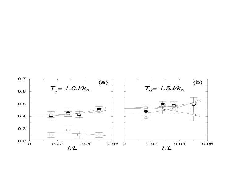
FIG. 9.: Exponents $x$ ($\bullet$) from the excess energy per site ($\Delta E$), $y$ ($\circ$) from the second moment of the radial scan of the superstructure peak $\sigma_{r}$ and $z$ ($\Box$) from the fitted amplitude of the transverse scan of the superstructure peak $\sigma_{t}$, as a function of $1/L$ with the atom-atom exchange mechanism. Data corresponds to temperature $T_{q}=1.0J/k_{B}$ (a) and $T_{q}=1.5J/k_{B}$ (b). Solid lines show the best fits of eq. (5.2).

FIG. 10.: Linear-log plot of the averaged transverse scan of the structure factor at different times and quenching temperatures $T_{q}=1.0J/k_{B}$ (a) and $T_{q}=1.5J/k_{B}$ (b) with the atom-atom exchange mechanism. Data correspond to systems of linear size $L=64$.

FIG. 11.: Linear-log and log-log (insets) plots of the scaled transverse scan of the structure factor at different times and quenching temperatures $T_{q}=1.0J/k_{B}$ (a) and $T_{q}=1.5J/k_{B}$ (b) with atom-atom exchange mechanism. Data correspond to systems of linear size $L=64$. The solid thick lines correspond to fits of expression (3.7) with $\alpha=1$ and $\sigma=1$. The dashed lines in the insets show the Porod’s law $\tilde{S}(\tilde{q})\sim\tilde{q}^{-4}$, while the solid lines show the slope of $\tilde{q}^{-2}$.

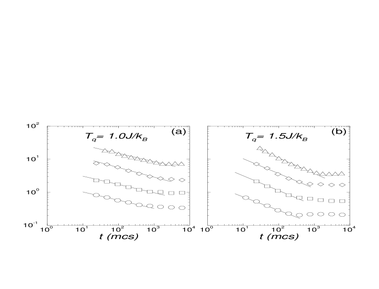
FIG. 12.: Log-log plot of the mean distance between type-1 walls for $L=20$ ($\circ$), $L=28$ ($\Box$), $L=36$ ($\Diamond$), $L=64$ ($\triangle$) with atom-atom exchange mechanism. Data correspond to quenching temperatures $T_{q}=1.0J/k_{B}$ (a) and $T_{q}=1.5J/k_{B}$ (b). Solid lines show the best power-law fits.

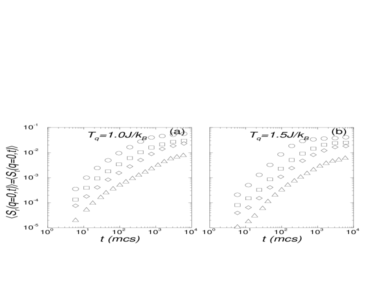
FIG. 13.: Log-log plot of the value of the structure factor at the superstructure peak $q=0$ for different system sizes ($L=20$ ($\circ$), $L=28$ ($\Box$), $L=36$ ($\Diamond$), $L=64$ ($\triangle$) and different quenching temperatures with the atom-atom exchange mechanism. The curves corresponding to different $L$ have been vertically shifted in order to clarify the picture.

FIG. 14.: Linear-log plot of the averaged radial scan of the structure factor at different times and quenching temperatures $T_{q}=1.0J/k_{B}$ (a) and $T_{q}=1.5J/k_{B}$ (b) for the vacancy-atom exchange mechanism. Both figures correspond to systems of linear size $L=64$.

FIG. 15.: Linear-log and log-log (insets) plots of the scaled radial scan of the structure factor at different times and quenching temperatures $T_{q}=1.0J/k_{B}$ (a) and $T_{q}=1.5J/k_{B}$ (b) for the vacancy-atom exchange mechanism. Data correspond to systems of linear size $L=64$. The solid thick line corresponds to a fit of expression (3.7) with $\alpha=1.5$ and $\sigma=1$. The dashed lines in the insets show the Porod’s law $\tilde{S}_{r}(\tilde{q})\sim\tilde{q}^{-4}$, while solid lines show the slope of $\tilde{q}^{-3}$.

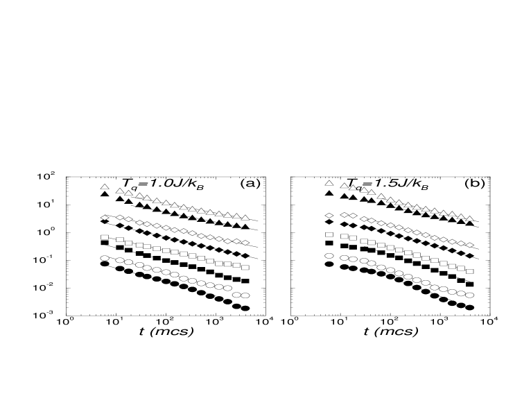
FIG. 16.: Time evolution, in the case of vacancy-atom exchange mechanism, of $\langle\Delta E(t)\rangle$ (filled symbols) and of $\sigma_{r}(t)$ (open symbols), for $T_{q}=1.0J/k_{B}$ (a) and $T_{q}=1.5J/k_{B}$ (b) for systems of $L=20$ (circles), $L=28$ (squares), $L=36$ (diamonds) and $L=64$ (triangles). The solid lines are the best power-law fits. Data corresponding to different sizes have been vertically shifted to clarify the picture.

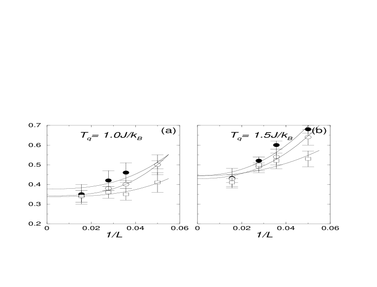
FIG. 17.: Exponents $x$ ($\bullet$) from the excess energy per site ($\Delta E$), $y$ ($\circ$) from the second moment of the radial scan of the superstructure peak $\sigma_{r}$ and $z$ ($\Box$) from the fitted amplitude of the transverse scan of the superstructure peak $\sigma_{t}$, as a function of $1/L$ with the vacancy-atom exchange mechanism. Data corresponds to temperature $T_{q}=1.0J/k_{B}$ (a) and $T_{q}=1.5J/k_{B}$ (b). Solid lines show the best fits of eq. (5.2).

FIG. 18.: Linear-log plot of the averaged transverse scan of the structure factor at different times and quenching temperatures $T_{q}=1.0J/k_{B}$ (a) and $T_{q}=1.5J/k_{B}$ (b) with the vacancy-atom exchange mechanism. Data correspond to systems of linear size $L=64$.

FIG. 19.: Linear-log and log-log (insets) plots of the scaled transverse scan of the structure factor at different times and quenching temperatures $T_{q}=1.0J/k_{B}$ (a) and $T_{q}=1.5J/k_{B}$ (b) with vacancy-atom exchange mechanism. Data correspond to systems of linear size $L=64$. The solid thick lines correspond to fits of expression (3.7) with $\alpha=1$ and $\sigma=1$. The dashed lines in the insets show the Porod’s law $\tilde{S}(\tilde{q})\sim\tilde{q}^{-4}$, while the solid lines show the slope of $\tilde{q}^{-2}$.

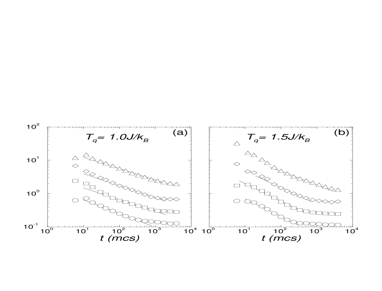
FIG. 20.: Log-log plot of the mean distance between type-1 walls for $L=20$ ($\circ$), $L=28$ ($\Box$), $L=36$ ($\Diamond$), $L=64$ ($\triangle$) with vacancy-atom exchange mechanism. Data correspond to quenching temperatures $T_{q}=1.0J/k_{B}$ (a) and $T_{q}=1.5J/k_{B}$ (b). Solid lines show the best power-law fits.

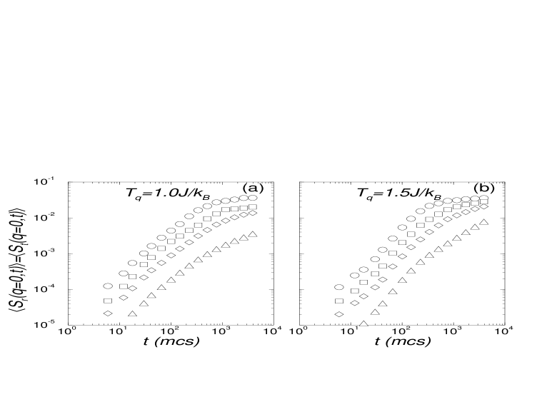
FIG. 21.: Log-log plot of the value of the structure factor at the superstructure peak $q=0$ for different system sizes ($L=20$ ($\circ$), $L=28$ ($\Box$), $L=36$ ($\Diamond$), $L=64$ ($\triangle$) and different quenching temperatures with the vacancy-atom exchange mechanism. The curves corresponding to different $L$ have been vertically shifted in order to clarify the picture.

FIG. 22.: Log-log plot of the structure factor decay in the radial ($\Box$), transversal($\triangle$) and diagonal ($\circ$) directions. Data, obtained with the atom-atom exchange mechanism, correspond to $t=1998mcs$, $T_{q}=1.0J/k_{B}$ and $L=64$.

TABLE I.: Directions of the non-energetic type-1 walls between possible pairs of neighboring domains.

$(\Psi_{1},\Psi_{2},\Psi_{3})$	$\alpha$ $(-1,-1,-1)$	$\beta$ $(-1,1,1)$	$\gamma$ $(1,-1,1)$	$\delta$ $(1,1,-1)$
$\alpha$		$[100]$	$[010]$	$[001]$
$\beta$	$[100]$		$[001]$	$[010]$
$\gamma$	$[010]$	$[001]$		$[100]$
$\delta$	$[001]$	$[010]$	$[100]$

TABLE II.: Fitted exponents of the power-law evolution of the excess energy per site ($\Delta E$), of the second moment of the radial scan ($\sigma_{r}$) and of the fitted amplitude of the transverse scan ($\sigma_{t}$). Data correspond to simulations with the atom-atom exchange mechanism.

$L$ $k_{B}T_{q}/J$	20	28	36	64	$L\rightarrow\infty$
1.0 $\Delta E$ $\sigma_{r}$ $\sigma_{t}$	$0.46\pm 0.02$ $0.44\pm 0.02$ $0.25\pm 0.03$	$0.41\pm 0.03$ $0.42\pm 0.03$ $0.25\pm 0.04$	$0.43\pm 0.03$ $0.42\pm 0.02$ $0.29\pm 0.02$	$0.40\pm 0.02$ $0.41\pm 0.02$ $0.25\pm 0.03$	$0.40\pm 0.02$ $0.41\pm 0.02$ $0.26\pm 0.02$
1.5 $\Delta E$ $\sigma_{r}$ $\sigma_{t}$	$0.50\pm 0.06$ $0.50\pm 0.05$ $0.41\pm 0.05$	$0.49\pm 0.03$ $0.48\pm 0.03$ $0.45\pm 0.04$	$0.50\pm 0.02$ $0.48\pm 0.03$ $0.45\pm 0.06$	$0.44\pm 0.03$ $0.39\pm 0.02$ $0.47\pm 0.05$	$0.46\pm 0.03$ $0.42\pm 0.02$ $0.47\pm 0.02$

TABLE III.: Fitted exponents of the power-law evolution of the excess energy per site ($\Delta E$), of the second moment of the radial scan ($\sigma$), and of the fitted amplitude of the transverse scan ($\sigma_{t}$). Data correspond to simulations with the vacancy-atom exchange mechanism.

$L$ $k_{B}T_{q}/J$	20	28	36	64	$L\rightarrow\infty$
1.0 $\Delta E$ $\sigma_{r}$ $\sigma_{t}$	$0.50\pm 0.02$ $0.50\pm 0.02$ $0.41\pm 0.03$	$0.46\pm 0.03$ $0.40\pm 0.03$ $0.35\pm 0.04$	$0.42\pm 0.03$ $0.38\pm 0.02$ $0.36\pm 0.02$	$0.35\pm 0.02$ $0.34\pm 0.02$ $0.34\pm 0.03$	$0.38\pm 0.02$ $0.34\pm 0.03$ $0.34\pm 0.02$
1.5 $\Delta E$ $\sigma_{r}$ $\sigma_{t}$	$0.68\pm 0.05$ $0.64\pm 0.03$ $0.53\pm 0.05$	$0.60\pm 0.05$ $0.54\pm 0.02$ $0.52\pm 0.04$	$0.52\pm 0.04$ $0.49\pm 0.02$ $0.50\pm 0.06$	$0.43\pm 0.05$ $0.43\pm 0.02$ $0.41\pm 0.05$	$0.44\pm 0.02$ $0.43\pm 0.01$ $0.44\pm 0.04$

TABLE IV.: Fitted coefficients $b$ of Eq. (5.2)

$k_{B}T_{q}/J$	atom-atom mechanism	vacancy-atom mechanism
$1.0$ $\Delta E$ $\sigma_{r}$ $\sigma_{t}$	98.7 45.4 -1271.5	386.1 1003.9 495.6
$1.5$ $\Delta E$ $\sigma_{r}$ $\sigma_{t}$	31.2 106.2 -34.7	212.3 233.3 88.4