[

Correlated ground states with (spontaneously) broken time-reversal symmetry

Abstract

We propose a self-consistent scheme for the determination of the ground-state (GS) properties of interacting electrons in a magnetic field, and of systems whose GS’s time-reversal-symmetry (TRS) is spontaneously broken. It is based on a newly-developed many-body perturbation theory that is valid, irrespective of the strength of correlation, provided the GS number densities $n_{\uparrow}({\bf r})$, $n_{\downarrow}({\bf r})$, and the total paramagnetic particle flux density are pure-state non-interacting $v$-representable. Our approach can in particular be applied to (modulated) two-dimensional electron systems in the fractional quantum-Hall regime.

]

Consider the following Hamiltonian that in the non-relativistic limit governs the behaviour of a general system of interacting electrons (we employ the SI units):

$$\widehat{H}{=} \sum_{\sigma}\int d^{3}r\;\widehat{\psi}_{\sigma}^{{\dagger}}({\bf r})\left\{{1\over 2m_{e}}\left[-i\hbar\mbox{\boldmath$\nabla$}+e\mbox{\boldmath$A$}({\bf r})\right]^{2}\right.$$ (2)

$$+\left.v({\bf r})+{1\over 2}g\mu_{B}B({\bf r})\sigma_{z}(\sigma)\right\}\widehat{\psi}_{\sigma}({\bf r})+\widehat{V},$$

with $\widehat{V}{=}(1/2)\sum_{\sigma,\sigma^{\prime}}\int d^{3}rd^{3}r^{\prime}$ $\widehat{\psi}_{\sigma}^{{\dagger}}({\bf r})\widehat{\psi}_{\sigma^{\prime}}^{{\dagger}}({\bf r}^{\prime})$ $v_{c}({\bf r}-{\bf r}^{\prime})$ $\widehat{\psi}_{\sigma^{\prime}}({\bf r}^{\prime})\widehat{\psi}_{\sigma}({\bf r})$ the interaction part (the quantities in these expressions are defined in Ref. [1]). Here for simplicity we have assumed that the magnetic field $\mbox{\boldmath$B$}({\bf r})\equiv\mbox{\boldmath$\nabla$}\wedge\mbox{\boldmath$A$}({\bf r})$, with $A$ the external vector potential, points in a definite direction, i.e. $\mbox{\boldmath$B$}({\bf r})=B({\bf r})\mbox{\boldmath$e$}_{z}$.

Efforts for determining the electron-electron interaction effects on the physical properties of systems described by $\widehat{H}$ include, e.g., use of the many-body perturbation theory at some level of approximation, various quantum Monte-Carlo techniques and exact-diagonalisation methods. Application of the (ordinary) perturbation theory is considered to be limited to so-called ‘weakly-correlated’ systems, and although suitable for dealing with ‘strongly-correlated’ systems, the latter two categories of mentioned methods are applicable only to systems consisting of relatively small number of particles or those whose Hilbert space is small. In this Communication we introduce a self-consistent many-body perturbation theory that, in principle, can be applied to weakly as well as strongly correlated systems. Here our attention will be mainly focussed towards some GS properties. In order to be able to describe GS’s with spontaneously broken TRS, we retain $A$ in Eq. (2) and identify the case of zero external magnetic field with $B({\bf r})\to 0$.

In a previous work [2] we have discussed a fundamental problem from which any perturbation theory can suffer: that despite the possible convergence of a perturbation series, the ultimate results may not even approximately be related to the quantities of interest. The reason for this type of breakdown of the perturbation theory lies in that the GS of the non-interaction Hamiltonian $\widehat{H}_{0}{=}\widehat{H}-\widehat{V}$ (possibly modified by some effective one-body term), may not be adiabatically connected with that of the fully interacting system [3].

Our analysis in Ref. [2] shows that a perturbation theory based on a non-interacting Hamiltonian $\widehat{H}_{0}^{{}^{\prime}}$ whose ground state $|\Phi_{0}^{{}^{\prime}}\rangle$ satisfies $\langle\Phi_{0}^{{}^{\prime}}|\widehat{{\cal O}}_{i}|\Phi_{0}^{{}^{\prime}}\rangle$ $=\langle\Psi_{0}|\widehat{{\cal O}}_{i}|\Psi_{0}\rangle$ ${\equiv}{\cal O}_{i}$, $i=1,2,\dots,{\cal N}$, with $|\Psi_{0}\rangle$ the GS of the fully interacting system and $\{\widehat{{\cal O}}_{i}|i=1,2,\dots,{\cal N}\}{\equiv}S_{\cal N}$ a specified set of quantities that uniquely determine the ground state of the system (see following paragraph), is an unconditionally valid perturbation theory [4]. We observe that for ${\cal O}_{i}$ $=\langle\Phi_{0}^{{}^{\prime}}|\widehat{{\cal O}}_{i}|\Phi_{0}^{{}^{\prime}}\rangle$ to be satisfied it is necessary that ${\cal O}_{i}$ be pure-state non-interacting $v$-representable (for definition see Ref. [5]).

For the work that we present in this Communication we rely on a theorem due to Vignale and Rasolt (VR) [6] according to which the GS of the Hamiltonian given in Eq. (2) is a unique functional of the number densities $n_{\sigma}({\bf r})$, $\sigma\in\{\uparrow,\downarrow\}$, and the total paramagnetic particle flux density $\mbox{\boldmath$j$}_{p}({\bf r}){=}\mbox{\boldmath$j$}_{p;\uparrow}({\bf r})+\mbox{\boldmath$j$}_{p;\downarrow}({\bf r})$. If the external vector potential $A$ were spin dependent, denoted by $\mbox{\boldmath$A$}_{\sigma}$, then the GS would become [6] a unique functional of $n_{\sigma}({\bf r})$ and $\mbox{\boldmath$j$}_{\sigma}({\bf r})$ for $\sigma=\uparrow,\downarrow$. To keep our approach general, so that both $\mbox{\boldmath$j$}_{p;\uparrow}$ and $\mbox{\boldmath$j$}_{p;\downarrow}$, pertaining to the interacting system, can be calculated [6], in what follows we formally assume to have a spin-dependent external vector potential; for the actual calculations we take $\mbox{\boldmath$A$}_{\uparrow}$ $\equiv$ $\mbox{\boldmath$A$}_{\downarrow}$ $\equiv$ $A$. Thus for the present case we have $S_{\cal N}$ $=S_{4}\equiv$ $\{\widehat{n}_{\sigma},$ $\widehat{\mbox{\boldmath$j$}}_{p;\sigma}|$ $\sigma=\uparrow,\downarrow\}$ in which $\widehat{n}_{\sigma}({\bf r})$ ${=}\widehat{\psi}_{\sigma}^{{\dagger}}({\bf r})\widehat{\psi}_{\sigma}({\bf r})$, and $\widehat{\mbox{\boldmath$j$}}_{p;\sigma}({\bf r})$ ${=}(-i\hbar/[2m_{e}])$ $\{\widehat{\psi}_{\sigma}^{{\dagger}}({\bf r})$ $[\mbox{\boldmath$\nabla$}\widehat{\psi}_{\sigma}({\bf r})]$ $-[\mbox{\boldmath$\nabla$}\widehat{\psi}_{\sigma}^{{\dagger}}({\bf r})]$ $\widehat{\psi}_{\sigma}({\bf r})\}$. The Hamiltonian $\widehat{H}_{0}^{{}^{\prime}}$ for the case at hand coincides with the Kohn-Sham (KS) Hamiltonian as introduced by VR [6]. We have $\widehat{H}_{KS}=\sum_{\sigma}\int d^{3}r\;\widehat{\psi}_{\sigma}^{{\dagger}}({\bf r})H_{KS;\sigma}({\bf r})\widehat{\psi}_{\sigma}({\bf r})$, in which [7]

$$H_{KS;\sigma}({\bf r}){\equiv} {1\over 2m_{e}}\left(-i\hbar\mbox{\boldmath$\nabla$}+e[\mbox{\boldmath$A$}({\bf r})+\mbox{\boldmath$A$}_{xc;\sigma}({\bf r})]\right)^{2}$$ (4)

$$-{{e^{2}}\over 2m_{e}}\left(A_{xc;\sigma}^{2}({\bf r})+2\mbox{\boldmath$A$}({\bf r})\cdot\mbox{\boldmath$A$}_{xc;\sigma}({\bf r})\right)$$

$$+v({\bf r}) +{1\over 2}g\mu_{B}B({\bf r})\sigma_{z}(\sigma)+v_{H}({\bf r})+v_{xc;\sigma}({\bf r}).$$ (5)

Let now $G_{\sigma}({\bf r}t,{\bf r}^{\prime}t^{\prime})$ denote the single-particle Green function corresponding to $\widehat{H}$, and $G_{KS;\sigma}$ that corresponding to $\widehat{H}_{KS}$. Making use of the results

$$\begin{array}[]{ll}n_{\sigma}({\bf r})=-iG_{\sigma}({\bf r}t,{\bf r}t+0^{+}),\\ \\ \mbox{\boldmath$j$}_{p;\sigma}({\bf r})={{-\hbar}\over 2m_{e}}\lim_{{\bf r}^{\prime}\to{\bf r}}\left(\mbox{\boldmath$\nabla$}-\mbox{\boldmath$\nabla$}^{\prime}\right)G_{\sigma}({\bf r}t,{\bf r}^{\prime}t+0^{+}),\end{array}$$ (6)

which, provided $n_{\sigma}$ and $\mbox{\boldmath$j$}_{p;\sigma}$ are pure-state non-interacting $v$-representable, are by construction also valid for $G_{\sigma}\to G_{KS:\sigma}$, and a perturbation expansion for $G_{\sigma}$ in terms of $G_{KS;\sigma}$, we obtain for a $d$-dimensional system a set of $2(d+1)$ coupled non-linear equations which we have diagrammatically represented in Fig. 1. From these equations the two $(d+1)$-vectors $(v_{xc;\sigma},\mbox{\boldmath$A$}_{xc;\sigma})$, $\sigma\in\{\uparrow,\downarrow\}$, can be determined and consequently the $\widehat{H}_{KS}$ on the basis of which an unconditionally valid perturbation theory can be set up [2]. The unfamiliar Feynman diagrams in Fig. 1 have their origin in the specific choice for the “unperturbed” Hamiltonian. For $\widehat{H}_{1}\equiv\widehat{H}-\widehat{H}_{KS}$ we have

$$\widehat{H}_{1} =-e\sum_{\sigma}\int d^{3}r\;\mbox{\boldmath$A$}_{xc;\sigma}({\bf r})\cdot\widehat{\mbox{\boldmath$j$}}_{p;\sigma}({\bf r})$$ (7)

$$- \sum_{\sigma}\int d^{3}r\;\widehat{\psi}_{\sigma}^{{\dagger}}({\bf r})\left\{v_{H}({\bf r})+v_{xc;\sigma}({\bf r})\right\}\widehat{\psi}_{\sigma}({\bf r})+\widehat{V}.$$ (8)

For casting $\widehat{H}_{1}$ into a form that makes application of the standard procedures of the many-body perturbation theory [8] possible, we define the following operator-valued non-local potential:

$$u_{xc;\sigma}({\bf r},{\bf r}^{\prime}){\equiv}{{ie\hbar}\over 2m_{e}}\delta({\bf r}-{\bf r}^{\prime})\mbox{\boldmath$A$}_{xc;\sigma}({\bf r})\cdot\left(\mbox{\boldmath$\nabla$}-\mbox{\boldmath$\nabla$}^{\prime}\right).$$ (9)

Through this the first term on the right-hand side of Eq. (7) can be written as $[-\sum_{\sigma}$ $\int d^{3}rd^{3}r^{\prime}$ $u_{xc;\sigma}({\bf r},{\bf r}^{\prime})$ $\widehat{\psi}_{\sigma}^{{\dagger}}({\bf r})\widehat{\psi}_{\sigma}({\bf r}^{\prime})]$. In Fig. 1 the directed wiggly lines, pointing from ${\bf r}^{\prime}\sigma$ to ${\bf r}\sigma$, stand for $(-i/\hbar)[-u_{xc;\sigma}({\bf r},{\bf r}^{\prime})]$. For the rules concerning evaluation of contribution of diagrams see Ref. [8].

Earlier Sham [9], by imposing $G=G_{KS}$ at ${\bf r}^{\prime}={\bf r}$, $t^{\prime}=t+0^{+}$ for systems of spin-less electrons (with no broken TRS), obtained an implicit expression for $v_{xc}$. Sham, however, did not address the problem concerning the validity of the many-body perturbation theory which is central to our present work.

Let the contributions of diagrams $(a_{1})$, $(b_{1})$ and $(c_{1})$ in Fig. 1 be denoted by $n_{\sigma}^{(x)}({\bf r})$ and $\mbox{\boldmath$j$}_{p;\sigma}^{(x)}({\bf r})$, with $x=a_{1},b_{1},c_{1}$. The non-linear equations associated with these first-order diagrams read (with $\sigma\in\{\uparrow,\downarrow\}$)

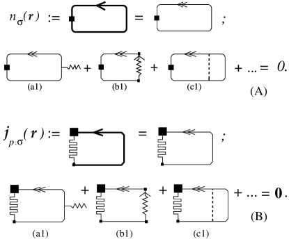
FIG. 1.: Diagrammatic representation of Eq. (6) with $G_{\sigma}$ (thick line with single arrow) and $G_{KS;\sigma}$ (double-arrowed thin line) on the right-hand sides (upper parts of (A) and (B)). Contributions of diagrams $(a_{1})$, $(b_{1})$, $(c_{1})$, $\dots$ add to zero for the correct $v_{xc;\sigma}$ (wiggly line with one loose end; the associated expression equals $(-i/\hbar)[-v_{xc;\sigma}]$) and ${\bf A}_{xc;\sigma}$ which defines $u_{xc;\sigma}$ (directed wiggly line) according to Eq. (9). The pulse-train-like line in (B) implies the non-local operation $(-\hbar/[2m_{e}])$ $\lim_{{\bf r}^{\prime}\to{\bf r}}$ $(\nabla-\nabla^{\prime})$ in Eq. (6). Lower parts of (A) and (B) correspond, respectively, to the first and the second equation in Eq. (10). Note that in first order only one diagram (i.e. $(c_{1})$) explicitly depends on the Coulomb interaction, represented by the broken line (corresponding to $(-i/\hbar)v_{c}$); this line can be taken to represent also the dynamically screened interaction function.

$$\begin{array}[]{ll}n_{\sigma}^{(a_{1})}({\bf r})+n_{\sigma}^{(b_{1})}({\bf r})+n_{\sigma}^{(c_{1})}({\bf r})=0,\\ \\ \mbox{\boldmath$j$}_{p;\sigma}^{(a_{1})}({\bf r})+\mbox{\boldmath$j$}_{p;\sigma}^{(b_{1})}({\bf r})+\mbox{\boldmath$j$}_{p;\sigma}^{(c_{1})}({\bf r})={\bf 0},\end{array}$$ (10)

in which

$$\begin{array}[]{ll}n_{\sigma}^{(x)}({\bf r})\equiv-2{\rm Re}\left\{\sum_{s}^{>}\sum_{s^{\prime}}^{<}U_{\sigma;s,s^{\prime}}^{(x)}\varrho_{\sigma;s^{\prime},s}({\bf r})\right\},\\ \\ \mbox{\boldmath$j$}_{p;\sigma}^{(x)}({\bf r})\equiv-2{\rm Re}\left\{\sum_{s}^{>}\sum_{s^{\prime}}^{<}U_{\sigma;s,s^{\prime}}^{(x)}\mbox{\boldmath$J$}_{\sigma;s^{\prime},s}({\bf r})\right\};\end{array}$$ (11)

$$\begin{array}[]{ll}U_{\sigma;s,s^{\prime}}^{(a_{1})}{\equiv}\int d^{3}r^{\prime}\;v_{xc;\sigma}({\bf r}^{\prime})\varrho_{\sigma;s,s^{\prime}}({\bf r}^{\prime})/(\varepsilon_{\sigma;s^{\prime}}-\varepsilon_{\sigma;s}),\\ \\ U_{\sigma;s,s^{\prime}}^{(b_{1})}{\equiv}e\int d^{3}r^{\prime}\;\mbox{\boldmath$A$}_{xc;\sigma}({\bf r}^{\prime})\cdot\mbox{\boldmath$J$}_{\sigma;s,s^{\prime}}({\bf r}^{\prime})/(\varepsilon_{\sigma;s^{\prime}}-\varepsilon_{\sigma;s}),\\ \\ U_{\sigma;s,s^{\prime}}^{(c_{1})}{\equiv}\sum_{s^{\prime\prime}}^{<}\int d^{3}r^{\prime}\;\varrho_{\sigma;s,s^{\prime\prime}}({\bf r}^{\prime})\\ \\ \times\left[\int d^{3}r^{\prime\prime}\;v_{c}({\bf r}^{\prime}-{\bf r}^{\prime\prime})\varrho_{\sigma;s^{\prime\prime},s^{\prime}}({\bf r}^{\prime\prime})\right]/(\varepsilon_{\sigma;s^{\prime}}-\varepsilon_{\sigma;s}),\\ \\ \varrho_{\sigma;s,s^{\prime}}({\bf r}){\equiv}\psi_{\sigma;s}^{*}({\bf r})\psi_{\sigma;s^{\prime}}({\bf r});\;\;\mbox{\boldmath$J$}_{\sigma;s,s^{\prime}}({\bf r}){\equiv}(-i\hbar/[2m_{e}])\\ \\ \;\;\;\times\{\psi_{\sigma;s}^{*}({\bf r})[\mbox{\boldmath$\nabla$}\psi_{\sigma;s^{\prime}}({\bf r})]-[\mbox{\boldmath$\nabla$}\psi_{\sigma;s}^{*}({\bf r})]\psi_{\sigma;s^{\prime}}({\bf r})\}.\end{array}$$ (12)

We have $n_{\sigma}({\bf r})=\sum_{s}^{<}\varrho_{\sigma;s,s}({\bf r})$, $\mbox{\boldmath$j$}_{p;\sigma}({\bf r})=\sum_{s}^{<}\mbox{\boldmath$J$}_{\sigma;s,s}({\bf r})$. For $\mbox{\boldmath$A$}\equiv\mbox{\boldmath$A$}_{xc}\equiv{\bf 0}$, the first equation in Eq. (10) reduces to one embodying the ‘optimised-potential method’ [10].

Above $\sum_{s}^{<}$ $(\sum_{s}^{>})$ stands for $\sum_{s=1}^{N_{\sigma}}$ $(\sum_{s=N_{\sigma}+1}^{\infty})$ and $\psi_{\sigma;s}$ denotes an eigenfunction of $H_{KS;\sigma}$ in Eq. (4), with $\varepsilon_{\sigma;s}$ the corresponding eigenvalue ($\varepsilon_{\sigma;s}$ $\leq$ $\varepsilon_{\sigma;s+1}$). Thus, Eq. (10) not only explicitly depends on $v_{xc;\sigma}$ and $\mbox{\boldmath$A$}_{xc;\sigma}$ (via Eqs. (11), (12)), but also implicitly, through $\{\psi_{\sigma;s},\varepsilon_{\sigma;s}\}$. Since in solving Eq. (10) we exactly diagonalise the KS Hamiltonian corresponding to any $(v_{xc;\sigma},\mbox{\boldmath$A$}_{xc;\sigma})$, the self-consistent $(v_{xc;\sigma},\mbox{\boldmath$A$}_{xc;\sigma})$ takes account of the electron-electron interaction effects, in so far as present in the employed diagrammatic expansion for $G_{\sigma}$, to infinite order. Moreover, it can be shown (cf. Ref. [2]) that a solution $(v_{xc;\sigma},\mbox{\boldmath$A$}_{xc;\sigma})$ of Eq. (10) based on a finite-order perturbation expansion for $G_{\sigma}$ annihilates the combined contributions to $n_{\sigma}$ and $\mbox{\boldmath$j$}_{p;\sigma}$ of all higher-order diagrams that have a common part in addition to one of the lower-order number-density diagrams (Fig. 1 (A)) that have been taken into account. Note that in solving Eq. (10), $N_{\uparrow}$ and $N_{\downarrow}$, satisfying $N_{\uparrow}+N_{\downarrow}=N_{e}$, must be calculated self-consistently: for a given $N_{e}$, $N_{\uparrow}$, or $N_{\downarrow}$, is determined by the requirement that $\varepsilon_{\uparrow;1},\dots,\varepsilon_{\uparrow;N_{\uparrow}}$, $\varepsilon_{\downarrow;1},\dots,\varepsilon_{\downarrow;N_{\downarrow}}$ are the lowest $N_{e}$ eigenvalues of $\{H_{KS;\sigma}\}$.

The non-linearity of Eq. (10) implies that there is a multiplicity of solutions. The uniqueness theorem of VR [6] implies, however, that only one of the solutions corresponds to the GS (solutions $\alpha+v_{xc;\uparrow}$, $\alpha+v_{xc;\downarrow}$, with $\alpha$ a constant, are identical). It is important that all solutions of Eq. (10) correspond to some [2] eigenstate of $\widehat{H}$. To single out the GS solution $(v_{xc;\sigma},\mbox{\boldmath$A$}_{xc;\sigma})$, let the GS of the system corresponding to the external potential $v=v_{0}$ and the external magnetic field strength $B=B_{0}$ (and therefore $\mbox{\boldmath$A$}_{0}$, in some gauge) be known. For the actual potential $v$ and magnetic field strength $B$ we define: $v^{(\lambda)}$ ${=}v_{0}$ $+\lambda(v-v_{0})$ and $\mbox{\boldmath$A$}^{(\lambda^{\prime})}$ ${=}\mbox{\boldmath$A$}_{0}$ $+\lambda^{\prime}(\mbox{\boldmath$A$}-\mbox{\boldmath$A$}_{0})$. For determining the GS solution of the non-linear equations we choose some trajectory on the $(\lambda,\lambda^{\prime})$-plane connecting $(0,0)$ with $(1,1)$. By starting from $(0,0)$, at small steps along the trajectory we solve Eq. (10) to self-consistency. In doing so, at each step we take the SC solution of the immediately earlier step as the trial solution. In the event of encountering degeneracy (level crossing at, say, $(\lambda_{0},{\lambda^{\prime}}_{0})$), we can easily select out the GS solution by realizing that at the point of degeneracy the energies of the degenerate states have discontinuous derivatives and the jump in the derivative of the GS total-energy curve is always negative and has the largest magnitude amongst the jump values corresponding to other energy curves. Now since the solutions found pertain to eigenstates of the Hamiltonian corresponding to $v^{(\lambda={\lambda}_{0})}$ and $\mbox{\boldmath$A$}^{(\lambda^{\prime}={\lambda^{\prime}}_{0})}$, we can apply the Hellmann-Feynman theorem [8], [2] which provides us with the derivatives of the eigenenergies with respect to $\lambda$ and $\lambda^{\prime}$. A simple calculation shows that $n_{\uparrow}^{(\lambda)}$, $n_{\downarrow}^{(\lambda)}$ and $\mbox{\boldmath$j$}_{p;\uparrow}^{(\lambda^{\prime})}+\mbox{\boldmath$j$}_{p;\downarrow}^{(\lambda^{\prime})}$ are sufficient for determining the mentioned derivatives [11]. Note that through integration of the available total-energy derivatives along the chosen path, the GS total energy is readily obtained.

FIG. 2.: Particle number and flux densities corresponding to a two-electron quantum dot in the $(M_{z},S_{z})$ state with $M_{z}$ and $S_{z}$, respectively, the orbital- and spin-angular momentum quantum numbers along the quantisation axis. The parameters chosen are those employed in Refs. [12],[13]: $B=1.0$ T, $v(r)=m_{e}^{*}\Omega^{2}r^{2}/2$ with $m_{e}^{*}=0.067m_{e}$ and $\Omega=3.37$ meV; $\epsilon_{r}=12.4$, $g=-0.44$; see Ref. [1]; the effective Bohr radius $a_{0}$ equals $9.794\times 10^{-9}$ m. The current density $-ej_{p;\sigma}(r)$, with $\sigma=\uparrow$, is in units of $2.95\times 10^{2}$ A/m (note the $-e$); $j_{p;\sigma}$, the azimuthal component of ${\bf j}_{p;\sigma}$ (the radial component is vanishing), corresponds to the symmetric gauge, ${\bf A}={\bf B}\wedge{\bf r}/2$.

Our proposed framework yields $n_{\sigma}$ and $\mbox{\boldmath$j$}_{p;\sigma}$ that exactly satisfy the static equation of continuity. This is because both of these are derived from the same single-particle Green function, $G_{KS;\sigma}$. Further, provided the ‘associated’ diagrams (see further on) corresponding to a particular order of the perturbation expansion for $G_{\sigma}$ are taken into account, our framework is also gauge invariant. To see this clearly, let the $4$-potential $(v_{xc;\sigma},\mbox{\boldmath$A$}_{xc;\sigma})$ correspond to $(v,\mbox{\boldmath$A$}_{\sigma})$. For definiteness suppose we have obtained the former by taking into account diagrams $(a_{1})$, $(b_{1})$ and $(c_{1})$ in Fig. 1, or by solving Eq. (10). Since $\mbox{\boldmath$A$}_{\sigma}\to$ ${\mbox{\boldmath$A$}^{\prime}}_{\sigma}\equiv\mbox{\boldmath$A$}_{\sigma}+\mbox{\boldmath$\nabla$}{\Lambda}_{\sigma}$ in a gauge-invariant theory must lead to $n_{\sigma}\to n_{\sigma}$ and $\mbox{\boldmath$j$}_{p;\sigma}\to\mbox{\boldmath$j$}_{p;\sigma}-(e/m_{e})n_{\sigma}\mbox{\boldmath$\nabla$}{\Lambda}_{\sigma}$, it follows that for $v_{xc;\sigma}^{\prime}$ and $\mbox{\boldmath$A$}_{xc;\sigma}^{\prime}$, corresponding to ${\mbox{\boldmath$A$}^{\prime}}_{\sigma}$, hold [6]: $v_{xc;\sigma}^{\prime}\equiv v_{xc;\sigma}$ $+(e^{2}/m_{e})$ $\mbox{\boldmath$A$}_{xc;\sigma}$ $\cdot\mbox{\boldmath$\nabla$}$ ${\Lambda}_{\sigma}$ and $\mbox{\boldmath$A$}_{xc;\sigma}^{\prime}$ $\equiv\mbox{\boldmath$A$}_{xc;\sigma}$. Our framework would be gauge non-invariant if Eq. (10) would not be satisfied by $(v_{xc;\sigma}^{\prime},\mbox{\boldmath$A$}_{xc;\sigma}^{\prime})$. We now show that this is not the case. First, $\varepsilon_{\sigma;s}$ does not depend on the choice of gauge. Further, from the explicit expressions in Eq. (12) it can be shown that $\varrho_{\sigma;s,s^{\prime}}$, similar to $n_{\sigma}$, is gauge invariant, and that for $\mbox{\boldmath$A$}_{\sigma}\to{\mbox{\boldmath$A$}^{\prime}}_{\sigma}$, $\mbox{\boldmath$J$}_{\sigma;s,s^{\prime}}$ $\to$ $\mbox{\boldmath$J$}_{\sigma;s,s^{\prime}}$ $-(e/m_{e})\varrho_{\sigma;s,s^{\prime}}$ $\mbox{\boldmath$\nabla$}\Lambda_{\sigma}$. It follows from Eq. (12) that $U_{\sigma;s,s^{\prime}}^{(a_{1})}$ $+U_{\sigma;s,s^{\prime}}^{(b_{1})}$ and $U_{\sigma;s,s^{\prime}}^{(c_{1})}$ are gauge invariant (diagrams $(a_{1})$ and $(b_{1})$ in Fig. 1 are ‘associated’). Thus $n_{\sigma}^{(a_{1})}$ $+n_{\sigma}^{(b_{1})}$ and $n_{\sigma}^{(c_{1})}$ are gauge invariant and $\mbox{\boldmath$j$}_{p;\sigma}^{(a_{1})}$ $+\mbox{\boldmath$j$}_{p;\sigma}^{(b_{1})}$ $\to$ $(\mbox{\boldmath$j$}_{p;\sigma}^{(a_{1})}$ $+\mbox{\boldmath$j$}_{p;\sigma}^{(b_{1})})$ $-(e/m_{e})$ $(n_{\sigma}^{(a_{1})}$ $+n_{\sigma}^{(b_{1})})$ $\nabla$ $\Lambda_{\sigma}$, $\mbox{\boldmath$j$}_{p;\sigma}^{(c_{1})}$ $\to$ $\mbox{\boldmath$j$}_{p;\sigma}^{(c_{1})}$ $-(e/m_{e})$ $n_{\sigma}^{(c_{1})}$ $\nabla$ $\Lambda_{\sigma}$. Therefore satisfaction of Eq. (10) does not depend on the choice of gauge.

We have applied our formalism to a cylindrically symmetric quantum dot with a parabolic confining potential, taking into account only the first-order diagrams that are explicitly shown in Fig. 1. In Fig. 2 we present the calculated electronic number and flux densities in the GS’s of definite symmetries (see caption) and compare the former with some available results [12],[13] — note that $\mbox{\boldmath$j$}_{p;\sigma}\equiv{\bf 0}$ in the $(M_{z}=0,S_{z}=0)$ GS. It turns out that in the $(1,1)$ state, our calculated $n$ $[\equiv n_{\uparrow}+n_{\downarrow}$; for the $(1,1)$ state, $n=n_{\uparrow}]$ is, within the numerical accuracy of the calculations, identical with the exact $n$. On the other hand, for small values of $r$ our $(0,0)$ GS $n(r)$ overestimates the exact $n(r)$ by several percents. Both of these density profiles are almost identical with the Hartree-Fock (HF) results [12]. There is however a fundamental difference between the HF results and those according to the present scheme. According to the HF approach, for all $B\not=0$, the GS of the system under consideration is a $(1,1)$ state, in obvious contradiction with the exact results [12]. For instance, for $B=1$T, the exact GS is a $(0,0)$ state, and the (first) transition to the $(1,1)$ state takes place at $B=2.0$T. In agreement with this, we find for $B=1$T the lowest-lying state to be a $(0,0)$ state. It should be mentioned that the results in Fig. 2 labelled by $(1,1)$ correspond to the lowest-energy $(1,1)$ state; for $B=1$T, as indicated, the state corresponding to the absolute minimum of energy is a $(0,0)$ state. It is therefore important to emphasise that the VR theorem [6] is also valid for excited states which are minimum-energy states corresponding to specified symmetries. This follows from the fact that the variational principle, which underlies the VR theorem, can also be applied in symmetry-restricted Hilbert spaces. For comparison, in Fig. 2 we present the results obtained within the local-density-approximation (LDA) scheme [13].

Concerning the overestimation in the vicinity of $r=0$ of our calculated $n(r)$ corresponding to the $(0,0)$ state, our preliminary calculations indicate that this is substantially suppressed through replacing $v_{c}$ in diagrams $(c1)$ of Fig. 1 by the dynamically-screened interaction function within the random-phase approximation.

We have analysed the asymptotic behaviour of the functions $v_{xc;\sigma}({\bf r})$, $\mbox{\boldmath$A$}_{xc;\sigma}({\bf r})$, for $|{\bf r}|\to 0,\infty$, corresponding to the system under consideration, both within the framework of the present formalism and that of the LDA. The results will be reported elsewhere [11]. We only mention that unless appropriate measures are taken, the current-carrying GS’s of the LDA [6] are unstable.

In conclusion, we have introduced a self-consistent perturbation theory for interacting electrons in presence or absence of an external magnetic field. In the latter case the system can possibly have a spontaneously broken TRS, such as is the case in open-shell atoms. Already the first stage in the application of this theory provides us with the scalar and vector exchange-correlation potentials that determine the Kohn-Sham Hamiltonian within the framework of the current-and-spin density-functional theory. This Hamiltonian forms the basis for construction of reliable perturbation expansions for various quantities, including those corresponding to the excited states of the interacting system, such as energies of the elementary excitations. We propose use of our method for determining properties of (modulated) two-dimensional electron systems in the fractional quantum-Hall regime where electrons are strongly correlated. Work in this direction is in progress.

The author should like to thank Professors Lars Hedin, Rolf Gerhardts, Vidar Gudmundsson, Drs Andrei Manolescu, Daniela Pfannkuche, and Professor Dieter Weiss for helpful discussions. The support of Max-Planck-Gesellschaft is gratefully acknowledged.

REFERENCES

[1]
In Eq. (2), and
, , are
creation and annihilation field operators; is the Landé factor,
the external potential (e.g., the confining potential),
the Bohr magneton; for ; , with
the electron charge, the vacuum permittivity
and the relative dielectric constant of the system. For
band electrons, the electron mass should be replaced by the
effective mass .
[2]
B. Farid, Phil. Mag. B 76, 145 (1997).
[3]
W. Kohn, and J. M. Luttinger, Phys. Rev. 118, 41 (1960).
[4]
Suppose were not adiabatically connected with
. Owing to the -representability of ,
it follows that the adiabatically-evolved is
the GS of some many-body that differs from
by non-trivial one-body terms (e.g., for
in Eq. (2), would involve and ,
with, e.g., differing by more than a constant from ). This
contradicts the fact that GS’s of such Hamiltonians cannot
[5] have identical .
[5]
R. M. Dreizler, and E. K. U. Gross, Density Functional Theory
(Springer, Berlin, 1990).
[6]
G. Vignale, and M. Rasolt, Phys. Rev. Lett. 59, 2360 (1987);
Phys. Rev. B 37, 10685 (1988).
[7]
In Eq. (4), is the Hartree potential, the exchange-correlation (XC) vector
potential, and the XC potential. For
details see Ref. [6].
[8]
A. L. Fetter, and J. D. Walecka, Quantum Theory of Many-Particle
Systems (McGraw-Hill, New York, 1971).
[9]
L. J. Sham, Phys. Rev. B 32, 3876 (1985).
[10]
J. D. Talman, and W. F. Shadwick, Phys. Rev. A 14, 36 (1976).
[11]
B. Farid, unpublished.
[12]
D. Pfannkuche, V. Gudmundsson, and P. A. Maksym, Phys. Rev. B 47,
2244 (1993).
[13]
M. Ferconi, and G. Vignale, Phys. Rev. B 50, 14722 (1994).