[

Spectral statistics near the quantum percolation threshold

Abstract

The statistical properties of spectra of a three-dimensional quantum bond percolation system is studied in the vicinity of the metal insulator transition. In order to avoid the influence of small clusters, only regions of the spectra in which the density of states is rather smooth are analyzed. Using finite size scaling hypothesis, the critical quantum probability for bond occupation is found to be $p_{q}=0.33\pm.01$ while the critical exponent for the divergence of the localization length is estimated as $\nu=1.35\pm.10$. This later figure is consistent with the one found within the universality class of the standard Anderson model.

]

The present work is concerned with level statistics in an Anderson type quantum percolation model. More specifically, we consider a single particle in a three-dimensional lattice with binary distribution of bonds and analyze (numerically) the distribution $P(s)$ of adjacent level spacings $s$ for bond occupation probabilities close to the critical one (which marks the metal insulator transition).

Level statistics in quantum systems and its relation to random matrix theories constitutes an important tool for understanding the underlying physics [1]. In particular, correlations between energy eigenvalues of a single quantum particle interacting with random impurities in the diffusive regime are consistent with the predictions of Gaussian matrix ensembles [2, 3, 4, 5, 6]. Recently, it became clear that in the vicinity of a metal insulator transition (provided it exists in such systems) there is a distinct kind of level statistics[7]. In this novel statistics, the critical exponent for the divergence of the localization length appears in numerous expressions for the various correlations[7, 8, 9, 10]. Hence, it is difficult to perceive a random matrix theory which adequately describe this critical statistics, although some progress has been recorded in this direction [11]. One of the clearest indications for the existence of a different statistics in the neighborhood of the metal insulator transition is displayed in the behavior of the nearest level spacing distribution $P(s)$, which, for large level spacing $s$, falls off slower than Gaussian [9]. This is found to be the case both for the Anderson metal insulator transition in three dimensions [12, 13] as well as for the Hall transition in two dimensions [14].

One of the motivations for studying level statistics in a quantum percolation model is related to the question of whether it belongs to the same universality class of the Anderson model with site disorder [15, 16]. The answer to this question is by no means clear, despite the fact that quantum percolation can be regarded as a special variant of the general Anderson model [17]. For example, in some quantum percolation models, the value of the critical exponent $\nu$ for the divergence of the localization length, as can be deduced from the transmission of the system, is found to be smaller than that of the Anderson model [18, 19]. Our analysis suggests that for a tight binding model the critical exponent (as can be deduced from the level statistics) for site disorder and that for quantum (bond) percolation are nearly identical.

Another motivation (upon which we will not elaborate in this work) concerns with the fractal nature of the wave function near the critical point. In particular, if the critical quantum probability for bond occupation (denoted hereafter as $p_{q}$) is only slightly higher than the classical one (denoted hereafter as $p_{c}$) then the critical wave functions live on a fractal object, and the geometrical fractal dimension becomes relevant.

Let us start by introducing the quantum percolation model and then explain how the nearest level spacing distribution is computed. Our calculations are based on a tight binding Hamiltonian,

$$H=\sum_{\langle ij\rangle}(t_{ij}a_{i}^{{\dagger}}a_{j}+h.c),$$ (1)

where $\langle ij\rangle$ denotes nearest neighbors. The hopping matrix elements $t_{ij}$ are independent random variables which assume the values $1$ or $0$ with probabilities $p$ and $q=1-p$ respectively. The underlying lattice is a three dimensional cube of length $L$ with periodic boundary conditions. The missing bond probability $q$ plays the role of disorder strength. For each realization $k$ of bond occupation probability, $p$, the above Hamiltonian is diagonalized exactly, yielding a sequence of eigenvalues $E_{n}^{k}$, $n=1,2,...L^{3}$. This sequence is calculated for $N$ different realizations, where $N=3000,1400,750,450,300$ for the corresponding different sample sizes $L=7,9,11,13,15$. This corresponds to $10^{6}$ eigenvalues for each sample size.

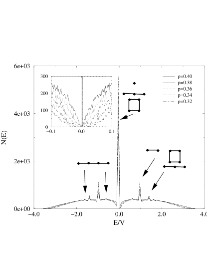
FIG. 1.: The DOS for $L=13$ as function of energy for different bond occupation values. The connection between various small clusters and peaks in the DOS are indicated in the figure. In the inset, an enlargement of the region around $E=0$ is presented.

The average density of states (DOS) for $L=13$ as a function of $p$ is presented in Fig. 1. The most noticeable feature is the appearance of a series of sharp peaks in the average DOS which increase as $p$ decreases. This feature was already noted in Ref. [20] where the DOS for a quantum percolating system was calculated using the Sturm sequence method. The origin of these peaks is the formation of small disconnected clusters of sites in the sample. For example, a single site with no connecting bonds to neighboring sites always contributes an eigenvalue $\varepsilon=0$. The probability for such a site is equal to $(1-p)^{6}$, therefore one expects a contribution of $L^{3}(1-p)^{6}$ eigenvalues equal to zero to the spectrum. This is in agreement[21] with the observed height of the central peak in Fig. 1 (the bin size is 0.072) and with its variation as function of $p$. Another prominent feature is the appearance of a gap in the DOS which depends on $p$ around the central peak [20] which may be seen in the inset of Fig. 1. A cluster of two sites connected by a bound has a probability of $p(1-p)^{10}$ to appear and contributes eigenvalues $\varepsilon=\pm 1$ to the spectra. Similarly, clusters of three sites contribute $\varepsilon=0,\pm\sqrt{2}$ and clusters of four sites contribute $\varepsilon=0,0,\pm\sqrt{2}$ if all the sites are connected among themselves and $\varepsilon=\pm(3\pm\sqrt{5})/2$ if only three bonds are present. It is interesting to note that gaps seem to develop also around these peaks.

Here we face the question of how to study a spectrum for which some of the levels form degenerate clusters. Indeed, one can apply the various statistical measures of level statistics only if the density of states is smooth. Looking at Fig. 1, one may concentrate on three such regions centered around (I) $E=\pm 0.4$, (II) $E=\pm 0.8$, (III) $E=\pm 1.2$ (the spectrum for an odd $L$ with periodic boundary conditions is not symmetric). In each region a fixed number of levels are taken ($15,31,57,95,145$ for $L=7,9,11,13,15$) and the spectrums unfolded by the usual procedure, i.e., $x_{i+1}=x_{i}+s_{i}$ and $s_{i}=n(E_{i+1}-E_{i})/(E_{i+\lfloor n/2\rfloor+1}-E_{i-\lfloor n/2\rfloor})$. In the data presented here $n=13$ is used, but no significant difference is seen for $n=9$. Within these guidelines, the distribution of adjacent level spacings for each region, sample size $L$ and bond probability $p$ is then calculated.

FIG. 2.: The level spacing distribution for $L=13$. One can see the transition from a GOE distribution (indicated by the thick full line) towards a Poisson distribution (indicated by the thick dashed line) as $p$ decreases.

A plot of P(s) as function of the bond occupation probability for $L=13$ is displayed in Fig. 2. It can be clearly seen that the expected transition from a Wigner like behavior for large $p$ to a Poisson behavior for small $p$ is manifested. One should also note that all curves seem to intersect at $s\sim 2$, which reminds us of the situation for the Anderson transition with on-site disorder[7]. As has been shown in Ref. [7] a very convenient way to obtain the mobility edge as well as the critical exponent of the transition $\nu$ is to study the parameter $\gamma(p,L)$ defined as

$$\gamma(p,L)={{\int_{2}^{\infty}P(s)ds-e^{-\pi}}\over{e^{-2}-e^{-\pi}}},$$ (2)

which characterizes the transition from Wigner to Poisson. Denoting by $\xi(p)$ the localization length, this function is expected to show a scaling behavior $\gamma(p,L)=f(L/\xi(p))$ which in the vicinity of the critical quantum bond probability $p_{q}$ is expected to behave as[7]

$$\gamma(p,L)=\gamma(p_{q},L)+C\left|{{p}\over{p_{q}}}-1\right|L^{1/\nu},$$ (3)

where $C$ is a constant. In Fig. 3 curves of $\gamma(p,L)$ for different sample sizes $L$ are plotted for levels in the first energy domain. It is noticed that the curves cross at a single point at which the order of heights with respect to $L$ is reversed. This is an indication for the existence of finite size one parameter scaling behavior. Similar situation prevails also in regions II and III.

FIG. 3.: The scaling function $\gamma$ as function of $p$ for different sample sizes for levels around $E=\pm 0.4$. A clear convergence of all curves at $p_{q}\sim 0.33$ can be seen, as well as the expected change in the size dependence of $\gamma$.

Based on finite size one parameter scaling analysis, the procedure for calculating the critical bond probability, as well as the critical exponent goes as follows. The quantity $\gamma(p,L)$ is calculated for many pairs $(p_{i},L_{i})$. It is then considered as a certain scaling function $f(x)$ of the scaling variable $x=L^{1/\nu}(p-p_{q})$. For $x\rightarrow\infty$ the system is well inside the diffusive regime and hence $f(x)\rightarrow 0$. On the other hand For $x\rightarrow-\infty$ the system is well inside the insulating regime and hence $f(x)\rightarrow 1$. Practically, it is useful to shift the variable $x$ to $y(x)=\frac{x-a-b}{b-a}$ where $a$ and $b$ are respectively the minimum and maximum values assumed by $x$. Evidently, $y(x)$ ranges between $-1$ and $1$. Then one expands $f(x)$ in a series of Tschebicheff polynomials $T_{n}[y(x)]$ ($n=0,1,2,...K$). Minimization of the set of differences $|f(x_{i})-\gamma(p_{i},L_{i})|$ results in the unknowns $p_{q}$, $\nu$ and the expansion coefficients (namely, the scaling function itself). In all cases, it is sufficient to cut off the number of polynomials at $K=12$.

The following results are obtained: for region I $p_{q}=0.335\pm.005$ and $\nu=1.32\pm.08$, for region II $p_{q}=0.33\pm.005$ and $\nu=1.35\pm.10$ and for region III $p_{q}=0.325\pm.005$ and $\nu=1.35\pm.12$. As a measure of the quality of the fit the numerical data and the fitted scaling function are plotted in Fig. 4. It can be seen that as one might expect $\nu$ is the same for all the three regions, while there is a small shift in $p_{q}$ as $E$ increases. The value of $p_{q}$ and its dependence on $E$ is in perfect agreement with previous numerical studies of quantum percolation systems [19, 20]. On the other hand, $\nu$ is not consistent with the different values of the critical exponent obtained for those systems, i.e.,$\nu=0.38$ in Ref. [18] and $\nu=0.75$ in Ref. [19], but is remarkably close to its value for the on-site disorder Anderson model [22, 7] $\nu=1.5\pm.1$.

FIG. 4.: A fit of the numerical data around $E=\pm 0.4$ to the scaling function represented by the curve.

Another quantity which is sensitive to the critical exponent $\nu$ is the behavior of the tail of $P(s)$ at the transition point. According to Kravtsov et. al [8] $\ln(-\ln(P(s)))=(2-\gamma)\ln(s)+{\rm const.}$, where $\gamma=1-{{1}\over{\nu d}}$. This is not an accurate algorithm to calculate $\nu$ since it depends on the behavior of $P(s)$ at the tail of the distribution, for which the statistics is rather poor. It is important to note that in Ref. [7] Shklovskii et. al predict $\gamma=1$ even in the critical region with no dependence on $\mu$ which is supported by some recent numerical work on the on-site Anderson model[23]. Nevertheless for the quantum percolation model we obtain $\gamma=0.68\pm.16$, which corresponds to $\nu=1.04^{+1.04}_{-.34}$. A better measure for $\gamma$ is the number variance $\Sigma^{2}(\bar{N})$ which should behave as $\Sigma^{2}(\bar{N})\propto\bar{N}^{\gamma}$, at least for moderate values of $N$ in which an additional linear term recently predicted[24] is not significant[14]. The logarithm of the number variance $\ln(\Sigma^{2}(\bar{N}))$ versus $\ln(\bar{N})$ is plotted in Fig. 5. Two different regions for which a linear behavior is observed can be seen (i) $1.5<\bar{N}<12$ and (ii) $20<\bar{N}<45$. In between, a jump in $\Sigma^{2}(\bar{N})$ can be seen which might be associated with some small cluster peak. A linear fit in (i) gives $\gamma=0.74\pm.02$ corresponding to $\nu=1.28^{+.11}_{-.09}$ and in (ii) $\gamma=0.76\pm.03$ resulting in $\nu=1.39^{+.20}_{-.16}$. All the above estimations of $\nu$ fall within the range obtained from the finite size one parameter scaling.

FIG. 5.: The logarithm of the number variance as function of the logarithm of the average number of states for the region around $E=\pm 0.8$. Linear fits were performed for (i) $1.5<\bar{N}<12$ and (ii) $20<\bar{N}<45$. For $12<\bar{N}<20$ a non monotonous behavior of the number variance is seen. This behavior is probably connected to a small peak in the DOS at $E\sim 0.83$.

Thus, based on the analysis of various statistical properties of the quantum percolation spectra, the critical exponent in the well behaved regions of the spectra is $\nu=1.35\pm.10$. This, at least for properties connected to the energy levels, seems to put the quantum percolation system in the same universality class as the usual on-site disorder Anderson model. The previous studies calculated $\nu$ via the transmission of the system at energies very close to $E=0$. As can be seen in the inset of Fig. 1 the DOS has a very strong $p$ dependence in that region. Thus a large part of the dependence of the transmission on $p$ is probably due to the change in the DOS and not because of some changes in the localization properties. Therefore, it will be very interesting to examine the transmission in regions of $E$ where the DOS has only a weak dependence on $p$.

We are grateful to D.E. Khmelnitskii and B. Shapiro for useful discussions. R.B. would like to thank the US-Israel Binational Science Foundation for financial support. Y.A. thanks the Israeli Academy of Science and Humanities for financial support.

REFERENCES

- [1] M. L. Mehta, Random matrices (Academic Press, San-Diego, 1991), and references therein.
- [2] L. P. Gorkov and G. M. Eliashberg Zh. Eksp. Teor. Fiz. 48, 1407 (1965) [Sov. Phys. JETP 21, 940 (1965)].
- [3] B. L. Altshuler and B. I. Shklovskii, Zh. Eksp. & Teor. Fiz. 91, 220 (1986) [Sov. Phys. JETP 64,127 (1986)].
- [4] U. Sivan and Y. Imry, Phys. Rev. B 35, 6074 (1987).
- [5] S. N. Evangelou and E. N. Economou, Phys. Rev. Lett. 68, 361 (1992).
- [6] F. M. Izrailev, Phys. Rep. 129, 299 (1990).
- [7] B. I. Shklovskii, B. Shapiro, B. R. Sears, P. Lambrianides, and H. B. Shore, Phys. Rev. B. 47, 11487 (1993).
- [8] V. E. Kravtsov, I. V. Lerner, B. L. Altshuler, and A. G. Aronov, Phys. Rev. Lett. 72, 888 (1994).
- [9] A. G. Aronov, V. E. Kravtsov and I. V. Lerner, JETP LEtt. 59, 39 (1994).
- [10] A. G. Aronov, V. E. Kravtsov and I. V. Lerner, Phys. Rev. Lett. 74, 1174 (1995).
- [11] M. Moshe, H. Neuberger and B. Shapiro, Phys. Rev. Lett. 73, 1497 (1994).
- [12] S. N. Evangelou, Phys. Rev. B 49, 16805 (1994).
- [13] E. Hofstetter and M. Schreiber, Phys. Rev. Lett. 73, 3137 (1994).
- [14] M. Feingold, Y. Avishai and R. Berkovits, Phys. Rev. B 52, 8400 (1995).
- [15] Y. Gefen, D. J. Thouless and Y. Imry, Phys. Rev. B 28, 6677 (1983).
- [16] B. Shapiro, Phys. Rev. Lett. 48, 823 (1982).
- [17] for a recent review see A. Mookerjee, I. Dasgupta and T. Saha, Int. J. Mod. Phys. 9, 2989 (1995), and references therein.
- [18] I. Chang, Z. Lev, A. B. Harris, J. Adler, A. Aharony, Phys. Rev. Lett. 74, 2094 (1995).
- [19] Y. Avishai and J. M. Luck, Phys. Rev. B 45, 1074 (1992).
- [20] C. M. Soukoulis, Q. Li and G. S. Grest, Phys. Rev. B 45, 7724 (1992).
- [21] Of course, one must take into account the fact that the central peak has contributions also from other clusters.
- [22] B. Kramer and A. MacKinnon, Rep. Prog. Phys. 56, 1469 (1993).
- [23] I. Kh. Zherekeshev and B. Kramer J. Jpn. Applied Phys. 34, 4361 (1995).
- [24] V. E. Kravtsov (preprint, cond-mat/9603166)