LUTTINGER LIQUIDS COUPLED BY HOPPING.

The stability of the Luttinger liquid to small transverse hopping has been studied from several points of view. The renormalization group approach in particular has been criticized because it does not take explicitly into account the difference between spin and charge velocities and because the interaction should be turned-on before the transverse hopping if the stability of the Luttinger liquid is a non-perturbative effect. An approach that answers both of these objections is explained here. It shows that the Luttinger liquid is unstable to arbitrarily small transverse hopping. The crossover temperatures below which either transverse coherent band motion or long-range order start to develop can be finite even when spin and charge velocities differ. Explicit scaling relations for these one-particle and two-particle crossover temperatures are derived in terms of transverse hopping, spin and charge velocities and anomalous exponents. The renormalization group results are recovered as special cases when spin and charge velocities are identical. The results compare well with recent experiments presented at this conference. Magnetic field effects are alluded to.

I Introduction.

The traditional approach to solid-state Physics relies on the existence of electronic elementary excitations that behave in many ways like non-interacting electrons. They are the “quasiparticles” of Landau Fermi liquid theory. Ever since Luttinger, it is known that in the case where interacting electrons move in one dimension, the Fermi liquid quasiparticles do not exist. Indeed, there are no simple fermionic eigenstates of the Hamiltonian that adiabatically connect with the non-interacting electrons, as in Fermi liquid theory. Instead, the excited eigenstates of the Hamiltonian become spin and charge collective modes (undamped paramagnons and zero-sound modes) each having their own linear dispersion relation and corresponding velocity. The single-particle Green’s function looses its single-particle pole in favor of a branch cut. Since the characteristic low-energy properties we have just described are displayed by a large class of microscopic models, the corresponding phenomenology has been given a generic name: Luttinger liquids.[1] The next section will remind the reader of key properties of electrons interacting in one-dimension.

In this conference proceedings, we study the problem of one-dimensional chains of interacting electrons, (Luttinger liquids) coupled by a perpendicular hopping amplitude $t_{\bot}$.This problem is of interest for several reasons. It is a reasonable model of quasi-one-dimensional conductors and possibly of coupled quantum wires that are discussed in this conference. Also, this problem can possibly lead to insights into the two-dimensional case that is of interest for high-temperature superconductors. More specifically, we address the question: Is there a finite critical value of $t_{\bot}$ below which the Luttinger liquid is stable at zero temperature? P.W. Anderson [2] has conjectured that when spin and charge velocities are different, then the answer to this question is yes. If there was such a critical value of $t_{\bot}$ below which the Luttinger liquid would survive, in the jargon we would say that we have “confinement”. The problem that we are studying is also known as the problem of “dimensional crossover”. Indeed, when the perturbation $t_{\bot}$ is zero, the system is clearly one-dimensional, while when the hopping parallel and perpendicular to the chains are equal, the system is clearly two-dimensional.

This question of the stability of the Luttinger liquid in the presence of $t_{\bot}$ has been addressed long ago in the context of quasi-one-dimensional conductors [3, 4, 5]. There it was shown that $t_{\bot}$ as well as pair-hopping correlations destabilize the Luttinger liquid fixed point. A series of recent works on two coupled chains [6] and on the many-chain problem [7] confirm this view but, nevertheless, the issue remains controversial [8]. In particular, going beyond the two chain case is a necessary requirement for phase transitions or long-range quasi-particle coherence to occur. The very few attempts to do so essentially deal with the situation where the spin and charge velocities are equal [4, 5]. To check Anderson’s conjecture, we must thus consider an approach where spin and charge velocities are different from the outset in the one-dimensional problem. Furthermore, again following Anderson’s suggestion, we must turn-on $t_{\bot}$ after the interaction, in such a way that we do start with fully correlated Luttinger liquids that are then coupled by a transverse hopping amplitude.

Since previous approaches do not satisfy the above two requirements, we start from a new functional integral formulation that does allow a systematic expansion in powers of $t_{\bot}$ using as the unperturbed system the Luttinger liquid with both anomalous exponents and differing spin and charge velocities. This allows us to generalize previous results and to understand in a unified way various limiting cases obtained before by several authors. We investigate both the single-particle spectral weight as well as the induced two-particle correlations.

Our results have appeared in various forms before[9][10]. We emphasize that, contrary to most previous investigations, we do not work at zero temperature. Instead, we consider the experimentally relevant situation where we start at finite temperature and study the stability of the Luttinger liquid as we decrease temperature. It should be intuitively clear that the Luttinger liquid is not destroyed by a perpendicular hopping when the temperature is much larger than the hopping integral $t_{\bot}\ll T$ ($k_{B}=1$) while remaining much smaller than the degeneracy temperature $T\ll E_{F}$. Indeed, in this limit the energy uncertainty brought about by thermal fluctuations does not allow one to detect the curvature of the Fermi surface that differentiates the quasi-one-dimensional case from the purely one-dimensional case. This is illustrated schematically in the figure below, drawn in the Brillouin zone of one-dimensional chains lying in a plane. On the left, we see the case where the spread in wave-vector caused by the thermal uncertainty $\Delta\epsilon_{{\bf k}}=\Delta\left(-2t_{\bot}\cos k_{\bot}a_{\bot}\right)\sim T$ corresponds to a wave vector uncertainty $\Delta k_{\bot}$ that is as large as the extent of the Brillouin zone in the direction perpendicular to the chains. Using the uncertainty principle, this means that the particles are essentially localized along the chains $1/\Delta k_{\bot}\sim a_{\bot}$, $\left(\hbar=1\right)$. The figure to the right shows the case where the temperature is low enough that the curvature of the Fermi surface becomes relevant. In the latter case, the nesting wave vector is the higher-dimensional one, contrary to the high-temperature case on the left where the nesting wave vector is one-dimensional.

FIG. 1.: The solid lines represent the Fermi surface of non-interacting one-dimensional electron chains coupled by a small perpendicular hopping. (From p.315 of Ref.[12]) The dashed line is the purely one-dimensional Fermi surface. The dotted lines represent a typical uncertainty in wave vector caused by thermal fluctuations. Nesting wave vectors have arrows. The nesting is one-dimensional on the left-hand side figure because $T>>t_{\bot}$. In this regime, the behavior is that of a Luttinger liquid. On the right-hand side figure, the nesting vector is two-dimensional because $T<<t_{\bot}$ .

Our main conclusions can be summarized as follows. For a given bare $t_{\bot}$ and temperatures much lower than the Fermi energy $T\ll E_{F}$, the typical crossover diagram that we find is sketched in Fig.2 as a function of temperature and of the anomalous exponent $\theta,$ the latter being taken as a measure of the interaction strength. As temperature is lowered, two types of crossovers can occur. For weak enough interaction, transverse one-particle coherent motion starts to develop, indicating that the crossover at the deconfinement temperature $T_{x^{1}}$ is from Luttinger liquid to Fermi liquid. This interpretation of $T_{x^{1}}$ is further reinforced by the infinite-range hopping model[11][10] where this result can be shown exactly. The one particle-crossover $T_{x^{1}}$ was studied before to two-loop order by Prigodin and Firsov[3] and to infinite order by Bourbonnais[3] and Schulz[13]. Moving on to strong interactions, virtual pair hopping becomes the dominating process which eventually leads to long-range ordering below the two-particle dimensional crossover temperature $T_{x^{2}}$, even if there is confinement at the one-particle level ($T_{x^{2}}\negthinspace>\negthinspace T_{x^{1}}$). At temperatures such that $0<$$T\negthinspace<T_{x^{1}}\left(T_{x^{2}}\right)$, a true phase transition can occur in more than two dimensions. It is important to notice that as long as there is no gap in the two-particle excitations, the crossover temperature $T_{x^{2}}$ increases with interaction strength, as shown in the figure. But when a gap appears, then the crossover temperature $T_{x^{2}}$ starts to decrease with interaction strength. This regime was studied by Brazovskii and Yakovenko[4]. The reason for the decrease with interaction strength can be understood by analogy with the Hubbard model at half-filling. In strong coupling, it maps onto the Heisenberg model but with an exchange constant $J$ that decreases with interaction strength as $J\sim t^{2}/U$.

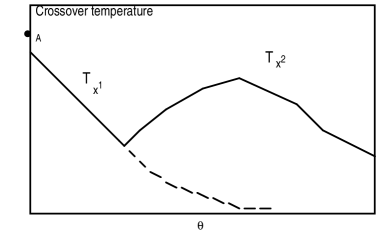
FIG. 2.: One-particle ($T_{x^{1}}$) and two-particle($T_{x^{2}}$) crossover temperatures shown qualitatively as a function of interaction strength schematically represented by $\theta$. The solid line becoming dotted indicates the one-particle deconfinement Luttinger liquid (LL)$\rightarrow$Fermi Liquid (FL) for the exact infinite-range transverse hopping model. Point A gives the non-interacting value of $T_{x^{1}}$ ($\sim t_{\bot}/\pi$) when $v_{\rho}=v_{\sigma}=v_{F}$.

It is clear that inasmuch as the crossover lines decrease to lower temperature with decreasing $t_{\bot}$ but without disappearing, then our results contradict those of Anderson. However, it is correct to say that it is possible to go from a Luttinger liquid to long-range order without ever becoming a Fermi liquid. We stress, furthermore, that our approach is strictly valid only above the crossover lines. While we can only conjecture, as above, what happens at temperatures below the crossover lines, we can, on the other hand, clearly state that the behavior is not that of a Luttinger liquid.

In the rest of this paper, we first recall some properties of the Luttinger liquid, in part to set the notation in the context of other presentations at this conference. Then we introduce our formalism and apply it to dimensional crossover at the one- and two-particle level ( $T_{x^{1}},T_{x^{2}}$). In the one-particle case, we briefly comment on the effect of a magnetic field.

II Some properties of the Luttinger liquid.

A One-particle properties

As a simple example of a Luttinger liquid, consider a Hamiltonian with electrons moving to the right or to the left with velocities $\pm v_{F}$. The kinetic energy is linear in the difference between the wave vector and the Fermi wave vector, and we assume that right-moving electrons interact only with right-moving electrons of opposite spin through a momentum independent two-body interaction $g_{4}$, and similarly for left-moving electrons. Then at zero temperature, the one-body Green’s function for right-moving electrons has the following asymptotic form

$$G_{+}\left(x,t\right)\sim\frac{e^{ik_{F}x}}{\sqrt{x-v_{\sigma}t}\sqrt{x-v_{\rho}t}}$$ (1)

where the $+(-)$ index to $G$ refers to right (left) moving electrons. The spin velocity $v_{\sigma}$ and the charge velocity $v_{\rho}$ are given by

$$v_{\sigma}=v_{F}\left(1-\frac{g_{4}}{2\pi v_{F}}\right)\quad;\quad v_{\rho}=\left(1+\frac{g_{4}}{2\pi v_{F}}\right)$$ (2)

The spectral weight, or probability that an electron of momentum ${\bf k}$ has an energy $\omega$ is given, for right-moving electrons, by

$$A\left({\bf k},\omega\right)=-\pi^{-1}{\rm Im}G_{+}^{R}\left({\bf k},\omega\right)=\frac{-1}{\pi}{\rm Im}\left[\frac{1}{\sqrt{\omega+i\eta-v_{\sigma}k}}\frac{1}{\sqrt{\omega+i\eta-v_{\rho}k}}\right]$$ (3)

Here, $k$ is measured with respect to the Fermi point. The spectral weight is schematically represented in the following figure. It is clearly qualitatively different from a Fermi liquid where we would see a peak representing a quasiparticle standing on a broad incoherent background.

FIG. 3.: Schematic representation of the spectral weight in the $g_{4}$ model

Note that the single-particle Green’s function Eq.(1) in real space factors into a part that comes from collective spin excitations and a part that comes from collective charge excitations. This qualitative feature is a characteristic of Luttinger liquids. This is what is meant by spin-charge separation.[13] In more general models, one will have power laws with interaction-dependent exponents instead of the square roots appearing in the simple $g_{4}$ model. The spin velocity and the exponent associated with spin will appear in one factor, while the charge velocity and the exponent associated with charge will appear in another factor. In fact, one of the factors, spin or charge, can even be gaped while the other is still described by a gapless spectrum.

The use of powerful techniques, such as the renormalization group, the Bethe ansatz, bosonization and conformal field theory techniques have allowed a quite thorough understanding of physical properties of Luttinger liquids.properties, such as the asymptotic low-energy behavior of the g-ology model, have been known for a long time[18][19][20]. By contrast, the calculation of asymptotic properties of correlation functions of the Hubbard model with and without magnetic field is relatively recent[21][22].

In the absence of either a spin or a charge gap, the most general form that the finite temperature one-particle Green’s function can take for right-moving electrons in a Luttinger liquid is [18][20][23][21]

$$G_{+}^{\left(1\right)}\left(x,\tau\right)=\frac{e^{ik_{F}^{0}x}}{2\pi i\Lambda^{\theta}}\prod_{\nu=\rho,\sigma}S\left(z_{\nu}\right)^{-1/2-\theta_{\nu}/2}S\left(z_{\nu}^{*}\right)^{-\theta_{\nu}/2}$$ (4)

where $S\left(z_{\nu}\right)\equiv\xi_{\nu}\sinh\left(z_{\nu}/\xi_{\nu}\right)$ and where naturally appears the complex coordinate $z_{\nu}=x+iv_{\nu}\tau,$ with $\tau$ the Matsubara time. The other symbols are the subscript $p=\pm$ to $G_{p}$ for the branch index and $\Lambda$ for the ultraviolet cutoff in wave number. The non-universal exponents $\theta_{\rho}>0$ and $\theta_{\sigma}>0$ are associated respectively with charge and spin, while the exponent without subscript, that we call the propagator’s anomalous exponent $\theta$, is simply $\theta=\theta_{\rho}+\theta_{\sigma}$. As before, $v_{\rho}$ et $v_{\sigma}$ are respectively the charge and spin velocities, while the associated thermal de Broglie correlation lengths are $\xi_{\rho,\sigma}=v_{\rho,\sigma}/\pi T$, $\left(\hbar=1\right).$ For values of space and imaginary time larger than these correlation lengths, the propagator falls-off exponentially, while for values much smaller than these lengths, it has a power law behavior, a phenomenology consistent with that of propagators close to a critical point. This critical point is at zero temperature since this is where the coherence lengths become infinite (Since the ratio of these lengths is a constant, there is only one of them that is relevant.) The existence of this zero-temperature critical point allows one to make full use of the renormalization group approach, as shown in Ref.[5].

Unfortunately, many different notations exist in this field. For the convenience of the reader, we mention that often in this conference the case of no magnetic anisotropy $\theta_{\sigma}=0$ was considered. Furthermore, the notation

$$\theta_{\rho}=\frac{1}{4}\left(K_{\rho}+K_{\rho}^{-1}-2\right)$$ (5)

was often used. Without attempting to be exhaustive, we give the following rosetta stone[9] (Table I) that may help the reader move through the literature. The first line is the notation used in the present work and in earlier ones by Bourbonnais.[5][11]

$\nu=(\sigma,\rho)$ exponent	Anomalous exponent	$\nu=(\sigma,\rho)$ velocities	References
$\theta_{\nu}$	$\theta$	$v_{\nu}$	this work
$\eta_{\nu}$	$\eta$	$u_{\nu}$	[7] ,[24]
$2\alpha_{\nu}$	$2\alpha$	$u_{\nu}$	[18]
$2\gamma_{\nu}=\left(K_{\nu}+K_{\nu}^{-1}-2\right)/4$	$2\gamma$	$u_{\nu}$	[25]
$\theta_{\rho}=\nu_{1}-1/2,\ \theta_{\sigma}=0$	$\nu_{1}-1/2$	$v_{c,s}$	[21],[22]
$\eta_{F\nu}-1/2=\left(\gamma_{\nu}+\gamma_{\nu}^{-1}-2\right)/4$	$\eta_{F}-1$	$v_{\rho,s}$	[26] ,[27]

TABLE I.: Connection between different notations for one-particle properties

B Two-particle properties

To study our problem, we will also need the asymptotic behavior of two-particle, or four point connected functions of the Luttinger liquid. By definition, omitting temporarily branch and spin indices, the four-point connected function is defined by

$$G_{c}^{\left(2\right)}\left(\left\{z\right\}\right)=G^{\left(2\right)}\left(\left\{z\right\}\right)+G^{\left(1\right)}\left(z_{1}-z_{4}\right)G^{\left(1\right)}\left(z_{2}-z_{3}\right)-G^{\left(1\right)}\left(z_{1}-z_{3}\right)G^{\left(1\right)}\left(z_{2}-z_{4}\right)$$ (6)

where $\left\{z\right\}=\left(z_{1},z_{2},z_{3},z_{4}\right)$ and, restoring indices,

$$G_{\left\{p,s\right\}}^{\left(2\right)}\left(\left\{z\right\}\right)=\left\langle T_{\tau}a_{p_{1}}^{s_{1}}\left(z_{1}\right)a_{p_{2}}^{s_{2}}\left(z_{2}\right)a_{p_{3}}^{s_{3}\dagger}\left(z_{3}\right)a_{p_{4}}^{s_{4}\dagger}\left(z_{4}\right)\right\rangle_{1D}$$ (7)

There are essentially three regimes with different asymptotic behavior. One weak-coupling regime, and two strong-coupling regimes. One of the strong coupling regime is gapless, while the other one has a gap. In the weak-coupling regime, the four-point function essentially scales as the product of two one-particle Green’s functions. Hence $\theta_{\rho}$ and $\theta_{\sigma}$ remain the only relevant exponents in this regime. By contrast, in the gapless strong-coupling regime, the four-point function scales as a product of composite bosonic operators. Hence, two new exponents appear, $\gamma_{\rho}$ and $\gamma_{\sigma}$. At even stronger coupling, a gap may appear in either the spin or the charge degrees of freedom. It is also important to realize that higher-order connected functions, $G_{c}^{\left(n\right)}$ for $n\geq 3,$ do not involve new exponents. Let us give the results for the two strong-coupling regimes.

1 Gapless strong-coupling regime.

The non-vanishing two-particle Green’s functions of a Luttinger liquid are of the form $G_{p,-p,-p,p}^{\left(2\right)}\left(z_{1}s,z_{2}s^{\prime},z_{3}s^{\prime},z_{4}s\right)$. Within logarithmic factors, their asymptotic form obtained from bosonization is[26][27]

$$G_{s,s^{\prime}}^{\left(2\right)}\left(\left\{z\right\}\right)\sim\Lambda^{-2\theta}\prod_{\nu=\rho,\sigma}\mid S\left(z_{1\nu}-z_{4\nu}\right)S\left(z_{2\nu}-z_{3\nu}\right)\mid^{-1/2-\theta_{\nu}}$$

$$\times\mid S\left(z_{1\nu}-z_{3\nu}\right)S\left(z_{2\nu}-z_{4\nu}\right)\mid^{-\delta_{\nu}(s,s^{\prime})}\mid S\left(z_{1\nu}-z_{2\nu}\right)S\left(z_{3\nu}-z_{4\nu}\right)\mid^{-\bar{\delta}_{\nu}(s,s^{\prime})}$$ (8)

where $\delta_{\rho}(s,s^{\prime})=\theta_{\rho}-\gamma_{\rho}/2+1/2=-\bar{\delta}_{\rho}(s,s^{\prime})$ (independent of $s,s^{\prime}$) for charge degrees of freedom, while for spin degrees of freedom, $\delta_{\sigma}(s=s^{\prime})=\theta_{\sigma}-\gamma_{\sigma}/2+1/2=-\bar{\delta}_{\sigma}(s=s^{\prime})$, and $\delta_{\sigma}(s\neq s^{\prime})=\theta_{\sigma}-\gamma_{\sigma}^{-1}/2+1/2=-\bar{\delta}_{\sigma}(s\neq s^{\prime})$. The exponents $\gamma_{\rho}$ and $\gamma_{\sigma}$ are functions of the microscopic interactions $g_{i\|},g_{i\bot}$. When there is no spin anisotropy, namely when $g_{i\|}=g_{i\bot}$, the spin-related exponent is $\gamma_{\sigma}=1$ while $\gamma_{\rho}$ is non-universal[18][23]. The relation to one-particle exponents is,[23]

$$\theta_{\nu}=\frac{1}{4}\left(\gamma_{\nu}+\gamma_{\nu}^{-1}-2\right)\text{.}$$ (9)

The gapless strong-coupling regime is defined as follows. Let us first consider the (repulsive) particle-hole channel. In strong coupling, the correlation function decays more rapidly than the inverse square of the relative particle-hole distances $\left|z_{1\nu}-z_{3\nu}\right|$ et $\left|z_{2\nu}-z_{4\nu}\right|$ so that the dominant asymptotic behavior is given by the relative distance between the two particle-hole pairs $z=z_{1}-z_{2}$. This situation is realized when $\delta_{\rho}\left(s,s^{\prime}\right)+\delta_{\sigma}(s,s^{\prime})>1$. For charge-density-wave (CDW) correlations, $s=s^{\prime}$, and one has $2\theta-\gamma_{\rho}-\gamma_{\sigma}>0$ whereas for spin-density-wave (SDW) correlations, $s\neq s^{\prime}$ and the strong coupling condition reads $2\theta-\gamma_{\rho}-\gamma_{\sigma}^{-1}>0$. The strong coupling condition for electron-hole correlations amounts to put $\left|z_{1\nu}-z_{3\nu}\right|\sim d_{\|}$ and $\left|z_{2\nu}-z_{4\nu}\right|\sim d_{\|}$ in the regime $\xi_{\nu}\gg d_{\|}\sim\Lambda^{-1}$, so that we have $\left|S\left(d_{\|}+id_{\|}\right)\right|\sim d_{\|}$. Using this result and the definitions

$$\gamma_{\mu}=2-\gamma_{\mu,\rho}-\gamma_{\mu,\sigma}$$ (10)

$\mu=0$ for CDW and $\mu\neq 0$ for SDW with $\gamma_{0,\rho}=\gamma_{\rho}$, $\gamma_{0,\sigma}=\gamma_{\sigma}$ and $\gamma_{\mu\neq 0,\rho}=\gamma_{\rho}$, $\gamma_{\mu\neq 0,\sigma}=\gamma_{\sigma}^{-1}$, we can write

$$G_{\mu}^{\left(2\right)}\left(z_{1}-z_{2}\right)\sim\Lambda^{\gamma_{\mu}}\prod_{\nu=\rho,\sigma}\left|S\left(z_{1\nu}-z_{2\nu}\right)\right|^{-\gamma_{\mu,\nu}},$$ (11)

($\Lambda^{\gamma_{\mu}}\sim$ $\Lambda^{-2\theta}d_{\|}^{-2\theta-\gamma_{\mu}})$. Note that this asymptotic behavior is the same as that of the response function $R_{\mu}\left(z\right)$ calculated in the same channel $\mu$[23][11]

$$R_{\mu}\left(z\right)\sim\Lambda^{\gamma_{\mu}}\cos 2k_{F}^{0}x\prod_{\nu=\rho,\sigma}\left[f_{\nu}\left(z_{\nu},z_{\nu}^{*}\right)S\left(z_{\nu}\right)S\left(z_{\nu}^{*}\right)\right]^{-\gamma_{\mu,\nu}/2}$$ (12)

where $f_{\nu}\left(z_{\nu},z_{\nu}^{*}\right)=2\left|z_{\nu}\right|^{2}\left[z_{\nu}^{2}+z_{\nu}^{*2}\right]^{-1}$ is a dimensionless function and where $z=z_{1}-z_{2}$ is the relative distance between pairs. The Fourier transform of (11) is well known to give rise to a power law singularity $R_{\mu}(2k_{F}^{0},T)\sim T^{-\gamma_{\mu}}$ in temperature. With the above definitions, the strong-coupling condition in the electron-hole channel can be written in the form

$$2-2\theta-\gamma_{\mu}<0$$ (13)

Similarly, strong attractive coupling in the electron-electron channel is achieved when $\bar{\delta}_{\rho}(s,s^{\prime})+\bar{\delta}_{\sigma}(s,s^{\prime})>1$, which for triplet superconductivity (TS), $s=s^{\prime}$ , corresponds to the condition $2\theta-\gamma_{\rho}^{-1}-\gamma_{\sigma}^{-1}>0$, while for singlet superconductivity (SS), $s\neq s^{\prime}$, it corresponds to the condition $2\theta-\gamma_{\rho}^{-1}-\gamma_{\sigma}>0$superconducting correlation and response functions [Eqs. (11)(12)] with $\gamma_{\mu=0,\rho}=\gamma_{\rho}^{-1},\gamma_{\mu=0,\sigma}=\gamma_{\sigma}$ for SS($\mu=0$) and $\gamma_{\mu\neq 0,\rho}=\gamma_{\rho}^{-1},\gamma_{\mu\neq 0,\sigma}=\gamma_{\sigma}^{-1}$ for TS($\mu\neq 0$). With these definitions of $\gamma_{\mu}$ in the particle-particle channel, the power law singularity in temperature of the response functions is again $R_{\mu}(T)\sim T^{-\gamma_{\mu}}$ with the same functional form for both Eq.(10) $\gamma_{\mu}=2-\gamma_{\mu,\rho}-\gamma_{\mu,\sigma}$ and the strong-coupling condition Eq.(13).

2 Strong-coupling regime with a gap.

A gap can open up for example at half-filling when umklapp scattering $g_{3}$ becomes relevant. Then, the charge excitations become gapped when[23] $\left|g_{3}\right|+2g_{2}-g_{1}>0$. The asymptotic form of the two-body correlation function in the presence of such a gap $\Delta_{\rho}$ is known[28]. We have been able to extract the result when spin and charge velocities differ. Let $l_{\rho}\sim v_{\rho}/\Delta_{\rho}$ be the size of a particle-hole pair. Then, when the distance between the particle and the hole forming a pair satisfies $\left|z_{1\rho}-z_{3\rho}\right|,\left|z_{2\rho}-z_{4\rho}\right|\ll l_{\rho}$, while the interpair distance is such that $\left|z_{1\rho}-z_{2\rho}\right|\gg l_{\rho}$ then the asymptotic form is

$$G^{\left(2\right)}\left(\left\{z\right\}\right)\sim\Lambda^{-2\theta}\frac{e^{-\left|z_{1\rho}-z_{3\rho}\right|/l_{\rho}-\left|z_{2\rho}-z_{4\rho}\right|/l_{\rho}}}{l_{\rho}^{1+2\theta_{\rho}}\left|S\left(z_{1\sigma}-z_{2\sigma}\right)\right|^{1+2\theta_{\sigma}}}\text{.}$$ (14)

Clearly, the thermal correlation length $\xi_{\rho}$ is replaced by the characteristic size of the pair $l_{\rho}$. Note that one can find an expression analogous to the last one, Eq.(14), when there is a gap $\Delta_{\sigma}$ in the spin channel, as may happen in the presence of attractive backscattering $g_{1}<0$.

As in the one-particle case, we present the (non-exhaustive) table II that should help the reader through the literature. The first line refers to the notation of Refs.[5][11] and of the present work.

$\nu=(\sigma,\rho)$ exponent	Susceptibility exponent	References
$\gamma_{\mu,\nu}$	$\gamma_{\mu}=2-\gamma_{\mu,\rho}-\gamma_{\mu,\sigma}$	this work
$\theta_{(c,s)}^{\mu}=\gamma_{\mu,(\rho,\sigma)}$	-	[23]
$\beta_{(c,s)}^{\mu}=\gamma_{\mu,(\rho,\sigma)}$	-	[18]
$\theta=4\gamma_{\mu,\rho},\gamma_{\mu,\sigma}=1$	-	[21] ,[22]

TABLE II.: Connection between different notations for two-particle properties

Note that in Refs.[18] and [23], the index $\mu$ means that $\beta_{c}^{0,1}=\beta_{c}$ and $\beta_{c}^{2,3}=\beta_{c}{}^{-1}$ while $\beta_{s}^{0,2}=\beta_{s}$ and $\beta_{s}^{1,3}=\beta_{s}{}^{-1}$.

III Formalism for dimensional crossover.

Let us start with the full partition function for a set of $N_{\bot}$ fully interacting chains written in the interaction representation where the unperturbed Hamiltonian is the complete interacting one-dimensional Hamiltonian

$${Z={\rm Tr}\{e^{-\beta\left(\sum_{i}{{\cal H}_{i}^{1D}}+\sum_{ij}{{{\cal H}_{\bot ij}}}\right)}\}=Z_{1D}\langle{T_{\tau}e^{-\int_{0}^{\beta}d\tau{\sum_{ij}}{\cal H}_{\bot ij}\left(\tau\right)}}\rangle_{1D}}$$ (15)

The indices $i,j$ run over all $N_{\bot}$ chains, ${\cal H}_{i}^{1D}$ is the purely $1D$ Hamiltonian describing the interacting electrons along chain $i$ while the interchain hopping part ${{{{\cal H}_{\bot ij}}}}$ stands as the perturbation. The above thermodynamic average $\langle{\ldots}\rangle_{1D}$ and partition function $Z_{1D}$ only involve the pure $1D$ Hamiltonian. The hopping Hamiltonian is given by ${{\cal H}_{\bot ij}=-\int dx\sum_{p,s}t_{\bot ij}{a_{p,i}^{s\dagger}}(x)a_{p,i}^{s}(x)}$ where $x$ is the continuous coordinate along the chains while $p=\pm$ denote right and left-going electrons as before. By analogy with the problem of propagation of correlations in critical phenomena, the propagation of one-particle transverse coherence is studied through an effective field theory which is generated by a Hubbard-Stratonovich transformation for Grassmann variables. This allows the partition function $Z$ to be expressed as a functional integral over a Grassmann $\psi^{\left(*\right)}$ field

$$Z=Z_{1D}\negthinspace\int\negthinspace\negthinspace\negthinspace\int{\cal D}\psi^{*}{\cal D}\psi\,e^{\;-\int d(1)\negthinspace\sum\limits_{ij}\psi_{i}^{*}(1)t_{\bot ij}^{-1}\psi_{j}(1)}{\langle\;e^{\;\int d(1)\negthinspace\sum\limits_{i}\left(a_{i}^{\dagger}(1)\psi_{i}(1)+\psi_{i}^{*}(1)a_{i}(1)\right)}\;\rangle_{1D}}$$ (16)

with the notations $\int d(n)\psi_{i}(n)\equiv\int dz_{n}\sum\nolimits_{p_{n},s_{n}}\psi_{p_{n},i}^{s_{n}}(z_{n})$ and $\int dz_{n}\equiv\int dx_{n}\int_{0}^{\beta}d\tau_{n}$. The logarithm of the thermodynamic average in (16) is readily recognized as the generating function for the exact $1D$ connected many-body Green’s functions $G_{c}^{(n)}$. Changing variables from $\psi_{i}$ to $\sum_{j}t_{\bot ij}^{1/2}\psi_{j}$ in the functional integral (16) allows us to obtain a field theory whose multipoint interactions involve successively higher powers of $t_{\bot}.$ We find

$${Z}=Z_{1D}\int\negthinspace\negthinspace\negthinspace\int{\cal D}\psi^{*}{\cal D}\psi\,e^{\,{\cal F}[\psi^{*},\psi]}$$ (17)

where the Grassmannian Landau-Ginzburg-Wilson functional ${\cal F}={\cal F}_{0}+\sum\nolimits_{n\geq 2}{\cal F}^{(n)}$ involves a quadratic part and a sum of effective interactions to all orders in the $\psi$ field. To write a specific form for ${\cal F}$, let us consider the case where chains are lined up in a plane and let us Fourier transform in the direction transverse to the chains. Then, the Gaussian part describing the free propagation of the $\psi$ field takes the form

$${\cal F}_{0}=-\int\negthinspace d(1)\negthinspace\int\negthinspace d(2)\negthinspace\sum\limits_{k_{\bot}}\psi_{k_{\bot}}^{*}(1)\left(\openone-t_{\bot}(k_{\bot})G^{(1)}(1-2)\right)\psi_{k_{\bot}}(2),$$ (18)

where $G^{(1)}$ is the exact one-dimensional propagator. The interacting part is found to be

$${\cal F}^{(n)}={\frac{1}{\left(n!\right)^{2}}\frac{1}{N_{\bot}^{n-1}}}\sum\limits_{k_{\bot 1}\ldots k_{\bot 2n}}\negthinspace\int\negthinspace d(1)\ldots\int\negthinspace d(2n)\psi_{k_{\bot 1}}^{*}(1)\ldots\psi_{k_{\bot 2n}}(2n)\gamma_{\bot}\left(k_{\bot 1}\ldots k_{\bot 2n}\right)G_{c}^{(n)}(1\ldots 2n)$$ (19)

where

$$\gamma_{\bot}\left(k_{\bot 1}\ldots k_{\bot 2n}\right)=\left\{\prod_{\alpha}^{2n}t_{\bot}\left(k_{\bot\alpha}\right)\right\}^{1/2}\delta_{\Sigma_{\alpha}k_{\bot\alpha},0}\ \;$$ (20)

in which $t_{\perp}(k_{\perp})$ is the Fourier transform of $t_{\perp ij}$. The Gaussian part gives the exact result in a few special cases: a) In the non-interacting limit $(G_{c}^{(n\geq 2)}\rightarrow 0)$ for arbitrary $t_{\bot}$ b) For arbitrary interaction when $t_{\bot}=0$. c) In the limit of infinite-range transverse hopping, whatever the value of $t_{\bot}$ and of the interaction[11][10]. Therefore $1/N_{\bot}$ may be used as a formal expansion parameter.

We will see that the crossover temperatures are those where the above functional integral approach ceases to be valid. Dimensional considerations like those presented below then lead to the following expansion parameters in the three regimes previously identified: a) in weak-coupling $g/\pi v_{F}\left[t_{\bot}/E_{F}^{\theta}T^{1-\theta}\right]^{2}$ with $g\ll\pi v_{F}$ the running coupling constant b) in the gapless strong (forward-scattering) coupling regime , $\left[t_{\bot}/E_{F}^{1-\gamma_{\mu}/2}T^{\gamma_{\mu}/2}\right]^{2}$ c) in the regime where there is, let us say, a charge $\Delta_{\rho}$ gap, $\left[t_{\bot}/E_{F}^{\theta}T^{1/2-\theta_{\sigma}}\Delta_{\rho}^{1/2-\theta_{\rho}}\right]^{2}$.

IV Dimensional crossover.

As described in the introduction, the Luttinger liquid may become unstable either at the one-particle or at the two-particle level. We describe these two cases in turn. In the one-particle case, we treat a simple example all the way to zero temperature, to suggest how a quasi-particle peak may develop. We also mention the results for the one-particle crossover in the case where a magnetic field is applied. For the explicit form of all dimensionless functions $F_{l}$ that appear in the following results for the crossover temperatures see Ref.[9].

A Single-particle dimensional crossover.

1 Zero magnetic field

An instability of the Luttinger liquid at zero temperature and thus the possibility of a Fermi liquid fixed point is already present in the free theory of the $\psi$ field described by ${\cal F}_{0}$. At this level of approximation, the $2D$ one-particle Green’s function in Fourier-Matsubara space, say for right-going electrons, is given by

$${\cal G}^{2D}({\bf k},\omega_{n})={\frac{{G^{(1)}(k,\omega_{n})}}{1-t_{\bot}(k_{\bot})G^{(1)}(k,\omega_{n})}},$$ (21)

where $\omega_{n}\negthinspace=\negthinspace(2n+1)\pi T$, while ${\bf k}=(k,k_{\bot})$ with $k$ measured with respect to the $1D$ Fermi point $k_{F}^{0}$. For the propagator $G^{(1)}$ describing the Luttinger liquid in space and imaginary time we can use our previous result Eq.(4). At high temperature, $t_{\bot}(k_{\bot})G^{(1)}(k,\omega_{n})\ll 1$ so that we have Luttinger liquid behavior. The one-particle propagator will definitely be different from that of a Luttinger liquid when the temperature is sufficiently low that $t_{\bot}(k_{\bot})G^{(1)}(k,\omega_{n})\sim 1$. Although we cannot strictly say towards what state the crossover will be as we decrease temperature, the following simple example suggests how a quasiparticle pole may appear, even when we have differing spin and charge velocities.

  A simple $T=0$ example.

Let us consider the Luttinger liquid Eq.(4) in the special case presented to introduce the Luttinger liquid Eq.(1). Then, $\theta_{\rho}\negthinspace=\negthinspace\theta_{\sigma}\negthinspace=\negthinspace 0$ but $v_{\rho}\negthinspace\neq\negthinspace v_{\sigma}$. In this case, we saw that the $T\negthinspace=\negthinspace 0$ retarded $1D$ propagator $G^{(1)}(k,\omega)$ has two square root singularities. At the Gaussian level, the corresponding spectral weight $A^{2D}=-\pi^{-1}{\rm Im}{\cal G}^{2D}$ obtained from the imaginary part of Eq.(21) is given by

$$A^{2D}({\bf k},\omega)={\frac{A^{1D}(k,\omega)}{{1+\left(\pi t_{\bot}(k_{\bot})A^{1D}(k,\omega)\right)^{2}}}}+Z(t_{\bot})\delta(\omega-\epsilon({\bf k))}$$ (22)

where $A^{1D}=-\pi^{-1}{\rm Im}G^{\left(1\right)}$ is the exact one-dimensional spectral weight, $Z\left(t_{\bot}\right)$ is the quasi-particle residue and $\epsilon\left({\bf k}\right)$ the pole of (21). For the case at hand, the undamped quasi-particle spectrum given by the pole of Eq.(21) is $\epsilon\left({\bf k}\right)=k\overline{v}$ $-{\rm sign}\left\{t_{\bot}\left(k_{\bot}\right)\right\}\sqrt{\left(k\Delta v\right)^{2}+t_{\bot}^{2}\left(k_{\bot}\right)}$ where $\overline{v}\negthinspace=\negthinspace\left(v_{\rho}+v_{\sigma}\right)/2$ and $\Delta v\negthinspace=\negthinspace\left(v_{\rho}-v_{\sigma}\right)/2$, while the quasi-particle residue takes the form

$$Z\left(t_{\bot}\right)=\frac{\left|t_{\bot}\left(k_{\bot}\right)\right|}{\sqrt{\left(k\Delta v\right)^{2}+t_{\bot}^{2}\left(k_{\bot}\right)}}.$$ (23)

The residue is readily seen to satisfy $Z\negthinspace\rightarrow\negthinspace 0$ when $t_{\bot}\negthinspace\rightarrow\negthinspace 0$ while $Z\negthinspace\rightarrow\negthinspace 1$ when $\Delta v\negthinspace\rightarrow\negthinspace 0$ as one expects for free electrons. Note that the infinite lifetime of the quasi-particles in Eq.(22) should become finite when one goes beyond the Gaussian approximation thus allowing the $\psi^{\prime}s$ to interact. This should be true except at the Fermi surface where the lifetime should remain infinite because of the usual phase space arguments. One can also check that for wave-vectors close to the new Fermi surface, given by $(v_{\rho}v_{\sigma})^{1/2}k=t_{\bot}(k_{\bot})$, the single-particle spectral weight has the following frequency dependence: For nearest-neighbor hopping and $k_{\bot}\negthinspace<\negthinspace\pi/2$, a quasi-particle peak is first encountered as the frequency is increased, followed by an incoherent background which is a smoothed version (without square-root singularity) of the original Luttinger liquid. In other words, remnants of spin-charge separation are left at high energies. This is illustrated qualitatively in the following figure which suggests that even if a Fermi liquid is recovered at low temperature, it is strongly renormalized with many properties that may be controlled by remnants of the Luttinger liquid. In fact, at $k_{\bot}\negthinspace=\negthinspace\pi/2$ there is not even a quasiparticle in this model.

FIG. 4.: Qualitative sketch of the zero-temperature spectral weight at fixed $k$, as function of frequency in the presence of $t_{\bot}$ for the simple model with only $g_{4}$ different from zero and $k_{\bot}<{\pi\over 2}$

In the more general case $\theta\negthinspace\neq\negthinspace 0$, we cannot repeat the above derivation to find $Z\left(t_{\bot}\right)$ analytically although we can prove from known $1D$ spectral weights [25] that the same reasoning would predict a pole in regions where the $1D$ spectral weight is zero, leading to results qualitatively similar to those just discussed. (End simple model)

To find the temperature scale $T_{x^{1}}$ at which the pole in ${\cal G}^{2D}$ becomes perceptible and transverse single-fermion coherence starts to develop, we use the natural change of variables $\tau^{\prime}=\pi T\tau$ and $x=(\xi_{\rho}\xi_{\sigma})^{1/2}x^{\prime}$ to evaluate the Fourier transform of the $1D$ Green’s function (4) at the Fermi level $G^{(1)}(0,\pi T)$. Substituting in the $2D$ Gaussian propagator Eq.(21) one readily finds

$$T_{x^{1}}\sim E_{F}\left({\frac{t_{\bot}}{E_{F}}}\right)^{1/\left(1-\theta\right)}\left({\frac{v_{F}}{v_{\rho}}}\right)^{\theta_{\rho}/\left(1-\theta\right)}\left({\frac{v_{F}}{v_{\sigma}}}\right)^{\theta_{\sigma}/\left(1-\theta\right)}F_{1}\left(\left\{{v_{\sigma}/v_{\rho}}\right\}^{1/2}\right)$$ (24)

where $F_{1}\left(x\right)$ is a temperature independent function that satisfies $F_{1}\left(x\right)=F_{1}\left(1/x\right)$ and which also depends on $\theta_{\rho,\sigma}$. As long as $\theta\negthinspace<\negthinspace 1$, or equivalently if $G^{(1)}(x)$ decays more slowly than $x^{-2}$, the coupling $t_{\bot}$ is relevant and $T_{x^{1}}$ is finite, although smaller than the non-interacting value $T_{x^{1}}\sim t_{\bot}/\pi$.[3, 5, 7] The condition $\theta\negthinspace<\negthinspace 1$ is satisfied for the Hubbard model with a non half-filled band where one has the exact result $\theta\negthinspace\leq\negthinspace{1/8}$ [29]. For more specialized 1D models (forward scattering only, half-filling, etc.) one can have the cases $\theta\negthinspace=\negthinspace 1$ and $\theta\negthinspace>\negthinspace 1$ where transverse hopping becomes marginal and irrelevant respectively. In these cases, transverse band motion does not develop and the electrons remain spatially confined along the chains at all temperatures. As seen from Eq.(24), the effect of $\Delta v\neq 0$ is to decrease the deconfinement temperature but not to make it vanish. The vanishing of $T_{x^{1}}$ is nevertheless expected for sufficiently strong coupling since spin and charge degrees of freedom must recombine for an electron to tunnel on a neighboring chain. Indeed, it can be shown that in the limit where the ratio of spin to charge velocities vanish, then the dimensionless function behaves as $F_{1}\left(\left\{v_{\sigma}/v_{\rho}\right\}^{1/2}\right)\stackrel{{\scriptstyle v_{\sigma}/v_{\rho}\rightarrow 0}}{{\sim}}\left\{v_{\sigma}/v_{\rho}\right\}^{1/2}$ leading in turn to $T_{x^{1}}\rightarrow 0$ when the condition $\theta_{\sigma}<\frac{1}{3}(1-\theta_{\rho})$ is also satisfied.

2 In a magnetic field.

Dimensional crossover in the presence of a magnetic field has been the subject of numerous studies recently[30]. To illustrate the wide applicability of our method, we just comment, in a few special cases, on the effect of a magnetic field on the one-particle dimensional crossover. Working in the Landau gauge, and using the Peierls substitution

$$t_{\bot}\rightarrow t_{\bot}\exp\left(\frac{ie}{c}\int{\bf A\cdot}d{\bf r}\right)\rightarrow t_{\bot}e^{iQx}$$ (25)

with $Q=ed_{\bot}B/c$, the condition for the dimensional crossover becomes

$$t_{\bot}\left|G_{p}\left(k_{F}-Q,i\pi T\right)\right|\sim 1$$ (26)

In the case of non-interacting electrons, this gives that the one-particle crossover temperature obeys

$$\left(\pi T_{x^{1}}^{0}\right)^{2}+\left(v_{F}Q\right)^{2}\sim t_{\bot}^{2}$$ (27)

For large enough magnetic field then ($Q_{c}^{0}=ed_{\bot}B_{c}/c=t_{\bot}/v_{F}$), the one-particle dimensional crossover does not occur. The electrons remain one-dimensional.

In the simple $g_{4}$ model, the magnetic field that leads to confinement is smaller.

$$Q_{c}=ed_{\bot}B_{c}/c=\frac{t_{\bot}}{\left(v_{\rho}v_{\sigma}\right)^{1/2}}=\frac{t_{\bot}/v_{F}}{\sqrt{1+\frac{g_{4}}{\pi v_{F}}}}$$ (28)

In other words, the Luttinger liquid in this case is easier to confine than free electrons.

B Two-particle dimensional crossover.

We now proceed beyond the Gaussian level by taking into account the ${\cal O}(t_{\bot}^{2})$ quartic term in the functional Eq.(19) which describes correlated transverse pair tunneling. We argue that the system will undergo a two-particle dimensional crossover towards CDW, SDW ordered states if the interaction is repulsive and SS or TS superconducting states if it is attractive. Focusing on the $2k_{F}^{0}$ particle-hole channel, (repulsive case) we rewrite the partition function at the quartic level as

$${Z}=Z_{1D}\langle{e^{\sum\limits_{\mu,q_{\bot}}\int\{dz\}O_{\mu,q_{\bot}}^{*}(z_{3},z_{1})\gamma_{\bot}(q_{\bot})R_{\mu}(\{z\})O_{\mu,q_{\bot}}(z_{2},z_{4})}}\rangle_{\psi^{*}\psi}$$ (29)

with the obvious notations $\{z\}\negthinspace=\negthinspace\{z_{1},z_{2},z_{3},z_{4}\}$ and $\langle\ldots\rangle_{\psi^{*}\psi}$ as the average with respect to ${\cal F}_{0}$. The composite fields ${\it O}_{\mu,q_{\bot}}(z_{3},z_{1})=N_{\bot}^{-{1/2}}\sum_{k_{\bot}}\sum_{\alpha\beta}\psi_{-,k_{\bot}}^{\alpha*}(z_{3})\sigma_{\mu}^{\alpha\beta}\psi_{+,k_{\bot}+q_{\bot}}^{\beta}(z_{1})$ describe CDW ($\mu\negthinspace=\negthinspace 0$) and SDW ($\mu\negthinspace=\negthinspace 1,2,3$) correlations. For nearest-neighbor hopping, we approximate the transverse pair tunneling amplitude as $\gamma_{\bot}(q_{\bot})\approx(2t_{\bot})^{2}\cos(q_{\bot}),$ where $q_{\bot}$ is the transverse momentum of the particle-hole pair, by setting the incoming momenta to $0$ or $\pi$ since this leads to the highest value for $T_{x^{2}}$. In the above, $\sigma_{0}^{\alpha\beta}=\delta^{\alpha\beta}$, $\sigma_{\mu=1,2,3}^{\alpha\beta}$ are the Pauli matrices and the $q_{\bot}$ independent function $R_{\mu}(\{z\})$ is the appropriate linear combination of connected four point functions corresponding to charge or spin fluctuations.

To examine the possibility of phase transition, we perform a Hubbard-Stratonovich transformation on the ${\it O}_{\mu}$ fields. Let $\zeta_{\mu,q_{\bot}}^{*}(z_{3},z_{1})$ be the complex field conjugate to ${\it O}_{\mu,q_{\bot}}(z_{3},z_{1})$. The partition function $Z$ then takes the form

$$Z=Z_{1D}\int\!\!\!\!\int{\cal D}\zeta^{*}{\cal D}\zeta\,e^{-\;\int\!\{dz\}\!\sum\limits_{\mu,q_{\bot}}\zeta_{\mu,q_{\bot}}^{*}(z_{3},z_{1})\bigl{(}\openone-\gamma_{\bot}(q_{\bot}){\mit R}_{\mu}(\{z\})\bigr{)}\zeta_{\mu,q_{\bot}}(z_{2},z_{4})+{\cal O}(\zeta^{4})}.$$ (30)

Softening of the $\zeta$ field first occurs for a value of $q_{\bot}\negthinspace=\negthinspace\pi$ corresponding to the usual staggered order. The temperature $T_{x^{2}}$ at which the $\zeta$ field softens must be greater than $T_{x^{1}}$ to retain its meaning as a two-particle crossover temperature. In a very rough manner of speaking, the Hubbard-Stratonovich transformation allows us write, by analogy with the one-particle case Eq.(21)

$${\cal G}_{2D}^{\left(2\right)}\sim{\frac{{G^{(2)}}}{1-t_{\bot}^{2}G_{c}^{(2)}}}$$ (31)

so that the two-particle crossover temperature occurs at $t_{\bot}^{2}G_{c}^{(2)}\sim 1.$ Let us be more precise.

In the weak-coupling regime, $2-2\theta-\gamma_{\mu}>0$, the correlator essentially scales as the square of the one-particle propagator (4) so that

$$T_{x^{2}}^{\mu}\sim T_{x^{1}}F_{3}^{\mu}\left(\left(v_{\sigma}/v_{\rho}\right)^{1/2},\left\{g\right\}\right).$$ (32)

where $\left\{g\right\}$ stands for the set of dimensionless electron-electron interaction vertices and $F_{3}^{\mu}(x,y)$ vanishes when either of its arguments vanishes. It is only for sufficiently weak coupling that $T_{x^{2}}<T_{x^{1}}$ and that deconfinement takes place.

In the gapless strong-coupling limit $2-2\theta-\gamma_{\mu}<0$ , we already know that the correlator $R_{\mu}(z_{1}-z_{3},z_{2}-z_{4},z_{1}-z_{2})$ decays faster than the square of the electron-hole separations $|z_{1}-z_{3}|$ and $|z_{2}-z_{4}|$ so that the scaling is determined by $z=z_{1}-z_{2}$ only, leading to the asymptotic form in Eq.(12). To show that the fast decay of $R_{\mu}(z_{1}-z_{3},z_{2}-z_{4},z_{1}-z_{2})$ leads effectively to a contraction of the two coordinates appearing in the Hubbard-Stratonovich field requires a discussion whose details appear in Ref.([9]). We find that in this regime the two-particle crossover temperature is given by

$$T_{x^{2}}^{\mu}\sim E_{F}\left({\frac{t_{\bot}^{2}}{E_{F}^{2}}}\right)^{1/\gamma_{\mu}}\left({\frac{v_{F}}{v_{\rho}}}\right)^{\gamma_{\mu,\rho}/\gamma_{\mu}}\left({\frac{v_{F}}{v_{\sigma}}}\right)^{\gamma_{\mu,\sigma}/\gamma_{\mu}}F_{2}^{\mu}\left(\left(v_{\sigma}/v_{\rho}\right)^{1/2}\right)\;$$ (33)

where $E_{F}\sim$ $\Lambda v_{F}$ while $\gamma_{\mu}$ is the susceptibility exponent $R_{\mu}(2k_{F}^{0},T)\sim T^{-\gamma_{\mu}}.$ The dimensionless function $F_{2}^{\mu}(x)$ vanishes at $x=0$.

The third and last regime is the strong-coupling regime with a gap. In the case of a charge gap, the asymptotic expression for the correlator is given by Eq.(14), from which we find

$$T_{x^{2}}^{\mu}\sim E_{F}\left({\frac{t_{\bot}^{2}}{E_{F}^{2}}}\right)^{\frac{1}{1-2\theta_{\sigma}}}\left(\frac{E_{F}}{\Delta_{\rho}}\right)^{\frac{1-2\theta_{\rho}}{1-2\theta_{\sigma}}}\left({\frac{v_{F}}{v_{\rho}}}\right)^{\frac{2+2\theta_{\rho}}{1-2\theta_{\sigma}}}\left({\frac{v_{F}}{v_{\sigma}}}\right)^{\frac{2+2\theta_{\sigma}}{1-2\theta_{\sigma}}}F_{5}^{\mu}\left(\theta_{\sigma}\right)\;$$ (34)

Clearly, the increase of the gap $\Delta_{\rho}$ with increasing coupling makes $T_{x^{2}}^{\mu}$ decrease with increasing coupling, as stated in the introduction, unless $\left(1-2\theta_{\rho}\right)/\left(1-2\theta_{\sigma}\right)<0$

The above expressions for the two-particle crossover temperature Eqs.(33)(32) and (34) reduce to the known results [3][5] when $v_{\rho}\negthinspace=\negthinspace v_{\sigma}$.

Higher-order vertices, ${\cal O}(t_{\bot}^{3})...$ involve higher-order connected functions $G_{c}^{(3)}...$ of the Luttinger liquid. As mentioned in the section on the Luttinger liquids, these functions do not contain any new relevant exponent, hence they do not change the above scaling results for either $T_{x^{1}}$ or $T_{x^{2}}$. In the latter case, higher-order connected functions modify mode-mode coupling terms included in the functional (30).

V Comparison with experiment.

The quasi one-dimensional compound $(TMTTF)_{2}Br$ at ambient pressure has a resistivity that increases rapidly below a resistivity minimum at a temperature $T_{\rho}$. This signals the opening of a charge gap. Klemme et al.[31] have measured this temperature $T_{\rho}$ as a function of pressure (diamonds on Fig.(5) below). The results are presented by Jérome at this conference. Using NMR, they have also measured the Néel temperature for magnetic order $T_{N}$ (squares) as a function of pressure. One should understand that increasing pressure increases the overlap between orbitals, hence it decreases the dimensionless coupling constants. This means that when one compares the data in Fig.(5) with the schematic representation of our results Fig.2, one should move from right to left in the experimental plot when the interaction increases on the theoretical plot. The qualitative agreement between theory and experiment is excellent. In particular, it is clear from the experiment that the decrease of $T_{N}$ with increasing interaction (decreasing pressure) starts only when the charge gap opens up. At higher pressures, when there is no resistivity minimum above the Néel temperature, $T_{N}$ always increases with decreasing pressure. The inset on the figure emphasizes the low temperature part of the diagram to make the maximum in Néel temperature more apparent.

FIG. 5.: From Klemme et al., Fig.2, Ref.[31], temperature for magnetic order $T_{N}$ (squares) as a function of pressure for $(TMTTF)_{2}Br$. The connection between the maximum in $T_{N}$ and the minimum in resistivity $T_{\rho}$ (diamonds) is apparent.

VI Conclusions.

Our theoretical conclusions have been summarized at the end of our introduction. We have further shown that they are consistent with recent experiments also discussed at this conference.[31] The one-particle crossover in the presence of a magnetic field has also been briefly discussed.

We thank M. Fabrizio and J. Voit for helpful discussions. This work was partially supported by the Natural Sciences and Engineering Research Council of Canada (NSERC), the Fonds pour la formation de chercheurs et l’aide à la recherche from the Government of Québec (FCAR) and (A.-M.S.T.) the Killam Foundation as well as the Canadian Institute of Advanced Research (CIAR). A.-M.S.T. would like to thank the Institute for Theoretical Physics, UCSB. Partial support was provided by the National Science Foundation under Grant No. PHY94-07194.

LIQUIDES DE LUTTINGER COUPLÉS. 

La stabilité du liquide de Luttinger en présence de saut interchaîne a été étudiée de plusieurs points de vue. L’approche basée sur le groupe de renormalisation a particulièrement été critiquée parce qu’elle ne tient pas compte explicitement de la différence entre vitesses de spin et de charge et aussi parce que si la stabilité du liquide de Luttinger est un effet non perturbatif alors il faut tenir compte des interactions avant d’inclure le saut interchaîne. Une approche qui répond à ces deux objections est décrite ici. Elle montre que le liquide de Luttinger est instable en présence de sauts interchaînes arbitrairement petits. Les températures de crossover sous lesquelles se développent soit un mouvement de bande cohérent, soit l’ordre à longue portée, peuvent être différentes de zéro même lorsque les vitesses de spin et de charge diffèrent. Des relations d’échelle explicites pour ces températures de crossover à une-particule ou à deux particules sont dérivées en fonction du saut interchaîne, des vitesses de spin et de charge et des exposants anormaux. On retrouve les résultats du groupe de renormalisation comme cas particulier où les vitesses de spin et de charge sont identiques. Les résultats se comparent favorablement à de récentes expériences présentées à cette conférence. On fait aussi allusion à certains effets des champs magnétiques.

REFERENCES

- [1] F. D. M. Haldane, Phys. Rev. Lett. 45, 1358 (1980); J. Phys. C 14, 2585 (1981); Phys. Lett. 81A, 153 (1981); Phys. Rev. Lett. 47, 1840 (1981).
- [2] P. W. Anderson, Phys. Rev. Lett. 64, 1839 (1990); Phys. Rev. Lett. 65, 2306 (1990); Phys. Rev. Lett. 67, 3844 (1991).
- [3] C. Bourbonnais et al., J. Physique Lett., 45, L755 (1984); V. N. Prigodin and Y. A. Firsov, Sov. Phys. JETP 49,369(1979); H. G. Schuster, Phys. Rev. B 13, 628 (1976); L.P. Gorkov and I.E. Dzyaloshinskii, Sov. Phys. JETP 40, 198 (1974).
- [4] S. Brazovskii and V. Yakovenko, Sov. Phys. JETP 62, 1340(1985).
- [5] C. Bourbonnais and L. G. Caron, Physica B143, 451(1986); Europhys. Lett., 5, 209(1988); Int. Journ. Phys. 5, 1033(1991).
- [6] M. Fabrizio, A. Parola and E. Tosatti, Phys. Rev. B 46, 3159(1992); M. Fabrizio and A. Parola, Phys. Rev. Lett. 70, 226(1992); A. Finkelstein and A.I. Larkin, Phys. Rev. B 47, 10461(1993); V. Yakovenko, JETP lett. 56, 5101(1992); A.A. Nerseyan, A. Luther, and F. V. Kusmartsev, Phys. Lett. A 176, 363(1993).
- [7] C. Castellani, C. Di Castro, and W. Metzner, Phys. Rev. Lett. 69, 1703 (1992).
- [8] D. G. Clarke, S. P. Strong, P.W. Anderson, Phys. Rev. Lett. 72, 3218(1994).
- [9] PhD Thesis, Daniel Boies, Université de Sherbrooke III-920 (1994) (unpublished).
- [10] Daniel Boies, C. Bourbonnais, and A.-M.S. Tremblay, Phys. Rev. Lett. 74, 968 (1995).
- [11] C. Bourbonnais, Ph.D thesis, Université de Sherbrooke, (1985), unpublished.
- [12] C. Bourbonnais, in Strongly Interacting Fermions and High Superconductivity, Les Houches, Session LVI, 1991, Eds. B. Douçot and J. Zinn-Justin (Elsevier, Amsterdam, 1995), p.307.
- [13] H. J. Schulz, Int. J. Mod. Phys. B 5, 57 (1991).
- [14] D. C. Mattis et E. H. Lieb, J. Math. Phys. 6, 304 (1965).
- [15] A. Luther et J. Peshel, Phys. Rev. B 9, 2911 (1974).
- [16] A. M. Finkelshtein, JETP Lett. 25, 73 (1977).
- [17] For a review, see J. Voit, Reports on Progress in Physics 58, p. 977 (1995).
- [18] J. Solyom, Adv. Phys. 28, 201 (1979).
- [19] J. M. Luttinger, J. Math. Phys. 4, 1154 (1963).
- [20] I. E. Dzyaloshinski et A. I. Larkin, Sov. Phys. JETP 38, 202 (1974).
- [21] H. Frahm et V. E. Korepin, Phys. Rev. B 42, 10553 (1990).
- [22] H. Frahm et V. E. Korepin Phys. Rev. B 43, 5653 (1991).
- [23] V. J. Emery in Highly Conducting One-Dimensional Solids, eds J. T. Devreese, R. P. Evrard et V. E. van Doren (Plenum 1979), p. 247.
- [24] C. Castellani, C. Di Castro, and W. Metzner, Phys. Rev. Lett.72, 316 (1994).
- [25] J. Voit, Phys. Rev. B 47, 6740(1993); Habilitationsschrift, Universität Bayreuth, 1993 (unpublished).
- [26] S. Brazovskii et V. Yakovenko, J. Physique Lett. (Paris) 46, p. L-111 (1985).
- [27] S. A. Brazovskii et V. M. Yakovenko, Sov. Phys. JETP 62, 1340 (1985).
- [28] H. Gutfreund and R. A. Klemm, Phys. Rev. B 14, 1073 (1976).
- [29] H. J. Schulz, Phys. Rev. Lett. 64, 2831(1990).
- [30] L. Hubert and C. Bourbonnais, Synthetic Metals, 55-57, 4231 (1993).
- [31] B.J. Klemme, S.E. Brown, P.Wzietek, G. Kriza, P. Batail, D. Jérome, J.M. Fabre, Phys. Rev. Lett. 75, 2408 (1995).