Chain length dependence of the polymer-solvent
critical point parameters

Abstract

We report grand canonical Monte Carlo simulations of the critical point properties of homopolymers within the Bond Fluctuation model. By employing Configurational Bias Monte Carlo methods, chain lengths of up to $N=60$ monomers could be studied. For each chain length investigated, the critical point parameters were determined by matching the ordering operator distribution function to its universal fixed-point Ising form. Histogram reweighting methods were employed to increase the efficiency of this procedure. The results indicate that the scaling of the critical temperature with chain length is relatively well described by Flory theory, i.e. $\Theta-T_{c}\sim N^{-0.5}$. The critical volume fraction, on the other hand, was found to scale like $\phi_{c}\sim N^{-0.37}$, in clear disagreement with the Flory theory prediction $\phi_{c}\sim N^{-0.5}$, but in good agreement with experiment. Measurements of the chain length dependence of the end-to-end distance indicate that the chains are not collapsed at the critical point.

PACS numbers 61.25.Hq, 64.70.Fx, 05.70.Jk

I Introduction and overview

When long flexible polymers are dissolved in a bad solvent there exists a critical temperature $T_{c}(N)$ of unmixing slightly beneath the $\Theta$-temperature (figure 1). At this critical temperature, the system phase separates into a very dilute (solvent rich) solution of collapsed chains and a semidilute (polymer rich) solution. The process is qualitatively described by the mean field theory of Flory [1], which predicts simple power laws for the chain length ($N$) dependences of $T_{c}(N)$ and the corresponding critical volume fraction $\phi_{c}(N)$:

$$T_{c}(N) = \Theta/(1+1/\sqrt{N})^{2}$$ (1)

$$\approx \Theta-2\Theta/\sqrt{N},\hskip 8.53581ptN\rightarrow\infty$$ (2)

$$\phi_{c}(N) = 1/(1+\sqrt{N})$$ (3)

$$\approx 1/\sqrt{N},\hskip 8.53581ptN\rightarrow\infty.$$ (4)

Another power law is predicted for the shape of the coexistence curve near $T_{c}(N)$:

$$\phi^{(2)}_{coex}-\phi^{(1)}_{coex}=2\hat{B}(N)\tau^{\beta},\hskip 5.69054pt\tau\equiv 1-T/T_{c}(N),$$ (5)

with a critical order parameter exponent $\beta$ and a chain length dependent critical amplitude $\hat{B}(N)$ given by

$$\beta=\beta_{MF}=1/2,\hskip 5.69054pt\hat{B}(N)\propto N^{-1/4}.$$ (6)

Further power laws describe the intensity of critical scattering, the associated correlation lengths and the interfacial tension etc [2, 3], but will not be considered here.

Notwithstanding the qualitative correctness of the Flory theory in predicting a phase separation, it should be emphasised that the exponent $\beta=\beta_{MF}=1/2$ in equation 6, as well as the powers of $N$ in equations 2–6 are mean field results, and thus cannot be expected to be quantitatively correct. More generally one expects that (we follow the notation of a recent experimental study [4])

$$\hat{B}(N) \propto N^{-x_{1}},$$ (7)

$$\phi_{c}(N) \propto N^{-x_{2}},$$ (8)

$$\Theta-T_{c}(N) \propto N^{-x_{3}},$$ (9)

where the mean field values of the exponents defined in equation 7 are

$$x_{1}^{MF} = 1/4,$$ (10)

$$x_{2}^{MF} = x_{3}^{MF}=1/2.$$ (11)

It is an interesting open question to ask what are the correct values of these exponents. While it is generally accepted from the “universality principle”[5], as well as experimental findings [4, 7, 8, 9, 10, 11, 12, 13], that the phase separation of polymer solutions falls in the same universality class as the three dimensional Ising model, so that [6]

$$\beta\approx 0.325,$$ (12)

the theoretical understanding of the exponents $x_{1},x_{2},x_{3}$ in equation 7 is rather limited. Experimental data have yielded the estimates [4, 7, 8, 9, 10, 11, 12, 13, 14]

$$x_{1} \approx 0.23-0.34,$$ (13)

$$x_{2} \approx 0.38$$ (14)

$$x_{3} \approx 0.47-0.50.$$ (15)

However, theoretical estimates for these exponents are still controversial. De Gennes [15] suggested that in the limit of large $N$, one has the same scaling behaviour as in mean field theory, i.e. the coexistence curve scales as

$$\phi_{coex}^{(2)}-\phi_{coex}^{(1)}=\frac{1}{\sqrt{N}}\tilde{\phi}(\sqrt{N}\tau),$$ (16)

Since $\phi(z)$ must behave for small argument $z$ as $\tilde{\phi}(z)\propto z^{\beta}$, this yields

$$x_{1}=(1-\beta)/2\approx 0.34,$$ (17)

which is roughly compatible with experiments. However, the scaling with $\sqrt{N}$ in equation 16 implies that $x_{2}=1/2$, which clearly disagrees with equation 13. Muthukumar [16] on the other hand, suggested that in a limit where ternary interactions are important, one should have different exponents, namely

$$x_{1}=x_{3}=2/9,\hskip 5.69054ptx_{2}=1/3.$$ (18)

Subsequently this problem has received further attention in the literature [3, 17, 18, 19, 20]. Recall that the scaling structure in equation 16 can be justified in terms of a Ginzburg criterion [21] if one assumes that the chain linear dimensions are ideal [15]. It then follows (remembering that the chain gyration radius enters as a critical amplitude prefactor in the mean-field power laws of the correlation length of the monomer density fluctuations), that the critical density $\phi_{c}(N)$ coincides (up to a universal prefactor) with the onset of the “semi-dilute” regime, where chains overlap significantly [15]. This assumption is plausible because of the vicinity to the $\Theta$-state ($T=\Theta,\phi\rightarrow 0$), where chains indeed behave ideally and the gyration radius scales as

$$R_{g}\propto N^{1/2},\hskip 5.69054ptT=\Theta,\hskip 5.69054pt\phi\rightarrow 0,\hskip 5.69054ptN\rightarrow\infty.$$ (19)

However the fact that for $T<\Theta$ and $\phi\rightarrow 0,N\rightarrow\infty$ chains are collapsed:

$$R_{g}\propto N^{1/3},\hskip 5.69054ptT<\Theta,\hskip 5.69054pt\phi\rightarrow 0,\hskip 5.69054ptN\rightarrow\infty,$$ (20)

implies that one does not really know how $R_{g}$ scales with $N$ at the critical point. Therefore it is tempting to generalize the scaling ansatz 16 as follows [19].

$$\phi_{coex}^{(2)}-\phi_{coex}^{(1)}=\frac{1}{N^{x_{4}}}\tilde{\phi}(N^{x_{4}}\tau).$$ (21)

Equation 13 is, of course, still consistent with the behaviour of the coexistence curve at fixed $\tau$ in the limit $N\rightarrow\infty$ [3]:

$$\phi_{coex}^{(1)}=0,\hskip 5.69054pt\phi_{coex}^{(2)}=\frac{3}{2}(1-T/\Theta),$$ (22)

if $\tilde{\phi}(z\rightarrow\infty)=\frac{3}{2}z$. Since for small $z=N^{x_{4}}\tau$, the scaling function must behave as $\tilde{\phi}(z)\propto z^{\beta}$ in order to comply with equations 5 and 12, we conclude that

$$\phi_{coex}^{(2)}-\phi_{coex}^{(1)}=N^{x_{4}(1-\beta)}\tau^{\beta},\hskip 5.69054ptx_{1}=x_{4}(1-\beta).$$ (23)

From renormalization group arguments, Cherayil [19] has suggested that the exponents $x_{2}$ and $x_{3}$ can be expressed in terms of the new exponent $x_{4}$ as

$$x_{2}=1-x_{4},\hskip 5.69054ptx_{3}=x_{4}.$$ (24)

This theory, however, does not yield a prediction for $x_{4}$ itself, and to fit some experimental data it was assumed that $x_{4}=0.62,x_{2}=0.38$ [19]. Kholodenko and Qian [18] have presented arguments that the exponent $x_{2}$ is not even a universal quantity. If the scaling relations of Cherayil (equation 23,24) hold, this would imply that $x_{1},x_{2}$ and $x_{3}$ are all system specific quantities, depending upon the material under consideration! Finally, we note that Muthukumar’s result, equation 18, disagrees with the above scaling relation $x_{1}=x_{3}(1-\beta)$, and thus the theoretical situation is clearly somewhat confusing.

In view of these problems and the difficulties of extracting all relevant information from experiments (one not only wishes to check the relations of equation 7 but also seeks to clarify how the chain span scales with $N$ at criticality), study of this problem by Monte-Carlo computer simulations techniques [22] is highly desirable. In fact there has been some previous work on this problem which considered the vapour-liquid phase diagram of alkane chains [23] and coarse-grained off-lattice polymer models (see e.g. [24, 25]). However the work of reference [23] considers the problem of estimating absolute values of $T_{c}(N)$ and $\phi_{c}(N)$ for a chemically realistic model of alkanes for small $N$ and does not address the universal properties of the limit $N\rightarrow\infty$. The Gibbs ensemble Monte-Carlo method of Panagiotopoulos [26, 27] allows an efficient estimation of the coexistence curve well below the critical point, but a precise estimation of critical point parameters is difficult in this framework.

An alternative approach for estimating critical point properties from simulations is based on finite-size scaling [28, 29]. This approach has been very successful for both symmetrical [31] and asymmetrical [32] polymer mixtures in conjunction with the bond-fluctuation lattice model [35] and semi-grand canonical ensemble simulation techniques [30]. These studies also relied on the use of histogram reweighting [33] and (in the asymmetric case) recent advances in disentangling order parameter and energy fluctuations near criticality in a finite-size scaling context [34].

In the present work we attempt to apply a related approach to study the liquid-vapour critical point of homopolymers within the Bond Fluctuation model. This problem is, however, somewhat more intricate than that of polymer mixtures since one must employ the grand canonical ensemble (GCE) [34] in order to effectively deal with the strong near-critical density fluctuations. As is well known, GCE simulations for chain molecules are extremely difficult, since the insertion probability for a polymer chain into a many chain systems is vanishingly small [22, 36, 37, 38]. For chains that are not too long (and/or systems that are not too dense), this problem can be eased by the Configurational Bias Monte-Carlo (CBMC) Method [36, 37, 38]. In the present paper we combine CBMC with histogram reweighting and a finite-size scaling analysis in its form extended to asymmetric systems [32, 34]. By this special combination of recent techniques (which will be briefly reviewed in section II) we are able, for the first time to obtain accurate results, both for $\phi(N)$ and $T_{c}(N)$ up to $N=60$ effective monomers. Since the effective bond in the bond-fluctuation model can be thought of as corresponding to $3$ to $5$ chemical bonds (when a mapping to chemically realistic chain molecules is attempted [35]), our simulations thus correspond to a degree of polymerization up to a few hundred chemical bonds along the chain backbone.

Section III then presents our results, including a highly precise estimation of the $\Theta$ temperature from an analysis of the gyration radius of simple isolated chains. We obtain both the location of the critical point in the $(T,\phi)$ plane as a function of chain length and, for the first time, the associated dependence of the chain span. In section IV we discuss our results and compare them to the theoretical ideas sketched above. We obtain very good agreement with experiment, but as in the latter the need to study much longer chains is clearly apparent to definitively clarify the true asymptotic behaviour for chain lengths $N\rightarrow\infty$.

II Algorithmic and computational aspects

The bond-fluctuation model (BFM) studied in this paper is a coarse-grained lattice-based polymer model that combines computational tractability with the important qualitative features of real polymers, namely monomer excluded volume, monomer connectivity and short range interactions. Within the framework of the model, each monomer occupies a whole unit cell of a 3D periodic simple cubic lattice. Neighboring monomers along the polymer chains are connected via one of $108$ possible bond vectors. These bond vectors provide for a total of $5$ different bond lengths and $87$ different bond angles. Thermal interactions are catered for by a short range inter-monomer potential. The cutoff range of this potential was set at $r_{m}=\sqrt{6}$ (in units of the lattice spacing), a choice which ensures that the first peak of the correlation function is encompassed by the range of the potential. We note also, that within our model, solvent molecules are not modelled explicitely, rather their role is play by vacant lattice sites. Further details concerning the BFM can be found in reference [35].

To implement a grand canonical ensemble simulation of the BFM, the Configurational Bias Monte Carlo (CBMC) method was employed [36, 37, 38]. The CBMC scheme utilizes a biased insertion method to ‘grow’ a polymer into the system in a stepwise fashion, each successive step being chosen so as to avoid excluded volume where possible. For brevity we shall merely outline the GCE implementation of this CBMC method and refer the reader to reference [40] for a fuller description.

Within the GCE scheme there are two complementary types of moves, insertion attempts and deletion attempts, both of which are made with equal frequency. An insertion move first involves attempting to grow a candidate polymer into the system. The basic strategy for achieving this is to insert successive monomers of the chain into the system one by one. The position of each successive monomer is chosen probabilistically from the set of $108$ possible BFM bond vectors emanating from the previously inserted monomer. The selection probability for each of the possible monomer positions is weighted by its Boltzmann factor, effectively biasing the choice in favour of low energy chain configurations. In order to keep track of the accumulated bias, a book keeping scheme is maintained. Once a candidate chain has been successfully grown, it is submitted to a Monte-Carlo lottery to decide whether or not it is to be accepted. The total chain construction bias is compensated for in the acceptance probability, thereby ensuring that detailed balance is obeyed.

For chain deletion moves, one chooses a chain at random from those in the system and ‘reconstructs’ its bias by examining the alternative growth scenarios at each step of the chain. The candidate chain for deletion is also submitted to a Monte-Carlo lottery to decide whether the proposed deletion should take place. As with the insertion lottery, the chain bias is taken into account in the deletion probability. The chemical potential, $\mu$, which controls the system chain density, also enters into the acceptance probability for both insertion and deletion.

The principal observables measured in the course of the simulations were the monomeric volume fraction:

$$\phi=8nN/V$$ (25)

and the dimensionless energy density:

$$u=8w^{-1}\Phi(\{r\})/V$$ (26)

where $n$ is the number of chains, $\Phi(\{r\})$ is the configurational energy, $w$ is the depth of the square well interaction potential (so that $T=w^{-1}$) and $V$ is the system volume. Here the factor of $8$ derives from the number of lattice sites occupied by one monomer in the BFM. Measurements of $\phi$ and $u$ were performed at intervals of $500$ chain insertion attempts and accumulated in the joint histogram $p_{L}(\phi,u)$. The final histograms comprised some $10^{5}$ entries. Also measured were the distributions of the chain radius of gyration and the chain end-to-end distances.

Using the GCE algorithm, chains of lengths $N=10,20,40,60$ were studied. For the $N=10$ and $N=20$ system size $V=40^{3}$ and $V=50^{3}$ were employed, while for $N=40$ and $N=60$ chain lengths only the $V=50^{3}$ was studied. Unfortunately it was not possible to study chains longer than $N=60$ since the acceptance rate for chain insertions falls exponentially with increasing $N$ and volume fraction $\phi$. This problem is illustrated in figure 2, where we plot the acceptance rate for a number of chain lengths as a function of the monomeric volume fraction. One sees for example, that for $N=80$ the acceptance rate is too low to provide reliable statistics within reasonable run times. Indeed, even for our longest chain length $N=60$, extremely long runs were required to gather adequate statistics.

Having outlined our model and simulation technique we now turn to a brief description of our data analysis methods. As mentioned in the introduction, finite-size scaling (FSS) methods are an indispensable tool for the proper treatment of critical behaviour, serving as they do to provide estimates infinite-volume critical properties from simulations of finite-size systems. The FSS methods we shall employ here are especially tailored to fluid systems and have been described in detail elsewhere [34]. The basic idea is to exploit the Ising character of the polymer liquid-vapor critical point to accurately locate the critical point. This is done by observing that precisely at criticality the distributions of certain readily measurable observables assume scale-invariant universal forms. The particular universal scaling form on which we shall focus, is the distribution of the ordering scaling operator $p_{L}({\cal M})$ . For the Ising model, the special symmetry between the coexisting phases implies ${\cal M}\rightarrow m$ (the magnetisation). The critical point form of $p_{L}(m)$ is independently known from extensive studies of large Ising lattices [39]. For fluids, however, the lack of symmetry between the coexisting phases implies [34] that the ordering operator is a linear combination of the fluid density and energy density i.e. ${\cal M}\rightarrow\phi+su$, where $s$ is a system specific ‘field mixing’ parameter that controls the strength of the coupling between the density and energy fluctuations.

Thus, in principle, one is able to accurately locate the critical point of a fluid system simply by tuning the $T,\mu$ and $s$ until the measured form of $p_{L}({\cal M})$ matches the known fixed point Ising form. In performing this task, the histogram reweighting method [33, 31] can be of great assistance. This technique allows one to generate estimated histograms $p_{L}(\phi,u)$ for values of the control parameters $T$ and $\mu$ other than those at which the simulations were actually performed. Such extrapolations are generally very reliable in the neighborhood of the critical point, due to the large critical fluctuations [33]. In what follows we shall detail the application of all these techniques to the problem of determining the liquid-vapor critical point parameters of our polymer model.

III Procedure and results

The first task undertaken was a determination of the $\Theta$-temperature for our model, knowledge of which is a prerequisite for studying the scaling of $\Theta-T_{c}(N)$ (cf. equation 7). To achieve this the gyration radius $R_{g}$ of single chains was studied as a function of temperature and chain length. From equations 19 one sees that precisely at the $\Theta$-temperature, and modulo corrections to scaling, $R_{g}^{2}/N$ should be independent of $N$. Extensive simulations were therefore carried out for single chains of length $N=64,80,100$ and $150$ at a temperature $T=2.0$. The full temperature dependence of $R_{g}$ for each chain length was subsequently obtained by histogram reweighting. This involves recording the joint histogram of the gyration radius and conformational energy of each configuration generated. The histogram for other temperatures may then be obtained by reweighting the Boltzmann factor for each histogram entry in the manner described in reference [33]. Figure 3 show the resulting curves of $R_{g}^{2}/N(T)$, which exhibit a very precise intersection point at $T=2.020(3)$, a value that we therefore adopt as our estimate of the $\Theta$-temperature.

In general for fluid systems, the coexistence curve is not known a-priori and must therefore be identified empirically as a prelude to locating the critical point itself. In the following we exemplify the general strategy for determining the critical parameters by considering the case of the $N=20$ system.

Initially a temperature of $T=1.75$ somewhat beneath the $\Theta$ temperature was chosen and the approximate value of the coexistence chemical potential was determined by tuning $\mu$ until $p_{L}(\phi)$ exhibited a double peaked structure. A long run was then carried out at this near-coexistence $\mu$ value, in which the histogram of $p_{L}(\phi,u)$ was accumulated. A histogram extrapolation based on this data was then used to extrapolate along the coexistence curve using the equal peak-weight criterion for $p_{L}(\phi)$ [41]. In this way a sizeable portion of the the near-critical coexistence curve (and its analytic extension[34]) could be located. Representative forms of the density distributions along this line of pseudo-coexistence are shown in figure 4(a), while the positions of the density peaks are shown in figure 4(b).

To locate the critical point along the line of phase coexistence, we utilized the universal matching condition for the operator distributions $p_{L}({\cal M})$ . Again applying the histogram reweighting technique, the temperature, chemical potential and field mixing parameter $s$ were tuned until the form of $p_{L}({\cal M})$ most accurately matched the universal fixed point Ising form $\tilde{p}^{\star}_{\cal M}(x)$. The results of performing this procedure are shown in figure 5 for the $V=40^{3}$ and $V=50^{3}$ system sizes. Given that these systems contain on average less than $100$ polymer chains at criticality, the quality of the data collapse is remarkable. The mappings shown were effected for a choice of the parameters $T_{c}=1.791(5),\mu_{c}=-5.16425(2),s=-0.135(4)$ where we have defined $\mu$ to be the chemical potential per monomer. The associated estimates for the critical volume fraction is $\phi_{c}=0.198(5)$. We note that this estimate of $T_{c}$ is rather less than what would be obtained, were one simply to extrapolate the liquid and vapour densities to the point at which they merge [figure 4(b)]. Thus our results further emphasise the finite-size errors that can arise using such a procedure.

We have also attempted to fit the coexistence curve data of figure 4(b), using fits of the Ising form: $\phi_{l}=\phi_{c}+0.745(T_{c}-T)+0.55(T_{c}-T)^{0.324},\phi_{v}=\phi_{c}+0.745(T_{c}-T)-0.55(T_{c}-T)^{0.324}$, with $T_{c}$ and $\phi_{c}$ assigned the values obtained above. For the Lennard-Jones fluid [42], a fit of this type gave a good description of the coexistence data for temperatures down to $0.8T_{c}$. Here, one sees that a reasonable fit can be obtained, but only for temperature within some $3\%$ of $T_{c}$. This would seem to suggest that the asymptotic Ising region in the polymer system is much smaller than in the Lennard-Jones system.

With regard to our estimates for the critical parameters, it should be emphasized that they are subject to errors arising both from corrections to scaling, as well as field mixing effects in the case of the critical volume fraction [34]. While in principal one can also correct for these effects, if one has access to a sufficient range of system sizes and ample statistics (see eg. [42]), the computational difficulties of the present problem preclude such an analysis. Indeed, for the $N=60$ system studied here, only one system size, $V=50$ was employed, this being the largest that could reasonably be tackled. Smaller system sizes were not studied since these would contain so few chains at criticality as to be excessively influenced by corrections to scaling. The matching to the universal form for the largest size available was then the only guide to the location of the critical point. Notwithstanding these problems however, we feel on the basis of our experience of corrections to scaling in other systems [42], that the quoted uncertainties generously encompass the infinite-volume critical parameters.

The procedure described above was repeated for the other chain lengths studied, allowing estimates to be obtained for $T_{c}(N)$ and $\phi_{c}(N)$. However the computational difficulty became progressively greater as $N$ increased, making the accumulation of good statistics problematic. As a result it was not possible to perform a reliable histogram extrapolation away from the critical point into the sub-critical two-phase region and thus no information on the $N$ dependence of the critical amplitude prefactor featuring in equation 7 could be obtained. An additional hindrance to probing the subcritical coexistence region is that the BFM appears to be unable to support a liquid phase for volume fractions $\phi\gtrsim 0.6$, instead collapsing into an amorphous crystal. This artifact is traceable to the limited conformational entropy of our lattice-based chains, and has also been observed in a previous study of tethered chains using the same model [43].

The results for $T_{c}(N)$ and $\phi_{c}(N)$ are plotted against $N^{-1}$ in figures 6 and  7 respectively. For $T_{c}(N)$ we find that the data can be well fitted by a Flory-type formula of the form $T_{c}=\Theta+a_{1}N^{-0.5}+a_{2}N^{-1}$ (where the $N^{-1}$ term can be thought of as a free-end correction and where we assume that $lim_{N\to\infty}T_{c}=\theta)$, although fits of the form $T_{c}(N)=\Theta+a_{1}N^{-x_{3}}$ yield a comparable fit quality for values of $x_{3}$ in the range $x_{3}=0.46$–$0.53$. For $\phi(N)$ we have performed a fit of the form $\phi_{c}(N)=(b_{1}+b_{2}N^{x_{2}})^{-1}$, and obtain $x_{2}=0.37(2)$.

Finally we have considered the $N$ dependence of the average squared end-to-end distance, $R_{ee}^{2}(N)$ at criticality. This quantity has been conjectured to scale as [19]:

$$R_{ee}^{2}(N)\propto N^{2\nu^{\prime}}$$ (27)

It was observed that the scaling of $\phi_{c}$ with $N$ could be explained if $\nu^{\prime}=0.46$, and we would like to check this conjecture. Our results are plotted in figure 8. Despite the very limited number of data points, we have attempted to fit this data to the form Eq. 27, with the result $R_{ee}^{2}(N)\propto N^{1.11(4)}$. This finding that $\nu^{\prime}>0.5$ is also supported by a study of the distribution function of end-to-end distances $p(r)$ at the estimated critical point. A scaling form for this function (valid for large $N$) may be written [44]

$$p(r)\propto r^{\kappa}\exp(-Dr^{\delta})$$ (28)

where $\delta\equiv(1-\nu)^{-1}$, $D$ is a constant and $\kappa=0.249\pm 0.011$ in three dimensions [44]. In figure 9 we plot the function $p(r^{2})r^{-0.1245}$ against $r^{2}$ on a logarithmic scale, for the chain length $N=40$ and $N=60$. Fits to the data yields estimates $\nu^{\prime}=0.51$ and $\nu=0.518$ respectively. Of course it is hard to believe that the chains are swollen at $T_{c}(N)$ which is below $\Theta$, given the fact that for $\phi\rightarrow 0$ at $T=\Theta$, the chains are not swollen. It is thus possible that the slight deviation from $\nu^{\prime}=1/2$ is simply due to corrections to scaling.

IV Discussion

In summary we have performed a study of the liquid-vapor critical point of a polymer model for chain lengths up to $N=60$ monomers. Owing to the low acceptance rate for chain transfers it was not possible to study either very long chains, or very large systems. Nevertheless we believe that the FSS-based technique we employed, of matching the measured scaling operator distribution functions to their fixed point universal forms is considerably more reliable than the practice of simply extrapolating a power law fit to coexistence curve data obtained well away from criticality, as has been the norm in previous simulation studies [23, 24, 27, 25]. Indeed, while we reproduce the previous results with regard to the finding that $T_{c}(N)$ is well described by a Flory formula, our measured value for the exponent $x_{2}=0.37(2)$, is in much closer accord with experiment ($x_{2}=0.38$) than previous simulation measurements. It is also interesting to note that for a similar range of monomeric units $N$, our coarse grained model seems to be much better at describing the asymptotic limit than chemically realistic models such as that employed in a the recent study of Alkanes [23], which did not even yield a monotonically decreasing $\phi_{c}(N)$.

With regard to the critical $N$ dependence of the chain span, our results suggest (albeit on the basis of a very limited number of data points) that the exponent $\nu^{\prime}>0.5$, which, if correct, would imply that the chains are slightly swollen at criticality—at variance with the suggestion of Cherayil [19, 46] and L’huiller [20] that $\nu^{\prime}\approx 0.46$, which is based on the assumption that the phase separation occurs when the chains just barely begin to overlap. We consider it possible, however, that our estimates for $\nu^{\prime}$ should be considered as effective exponents, which exceed the classical value $\nu^{\prime}=1/2$ only because of corrections to scaling. But in any case there is no evidence that the chains are somewhat collapsed at criticality.

Finally we remark that there is evidently a need to study longer chain and larger system sizes in order both to validate the results thus far obtained and to confirm that the limiting scaling behaviour is being observed. In view of the low acceptance rates for chain transfers at large $N$, algorithmic improvements are clearly necessary before this can be achieved. In this regard, recent improved biased growth techniques for chain insertion at large $N$ and $\phi$ promise to be extremely helpful [45]. In future work we hope to report on their application to the present problem.

Acknowledgements

The authors thank M. Muthukumar for a helpful discussion. NBW acknowledges financial support from the Max Planck Institut für Polymerforschung, Mainz. Part of the simulations described here were performed at the IWR, Universität Heidelberg. Partial support from the Deutsche Forschungsgemeinschaft (DFG) under grant number Bi314/3-2 and from the Bundesministerium für Bildung, Wissenshaft, Forschung und Technologie (BMBF) under grant number O3N8008C, is also gratefully acknowledged.

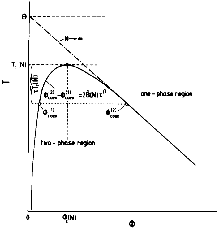
FIG. 1.: Schematic phase diagram of a polymer solution in the space of the temperature $T$ and the volume fraction $\phi$. The ceoxistence curve separates a dilute solution of collapsed chains [at $\phi^{(1)}_{coex}$] from a semildilute solution of overlapping chains [at $\phi^{(2)}_{coex}$]. These two branches of the coexistence curve merge at a critical point $T_{c}(N),\phi_{c}(N)$. For $N\rightarrow\infty$ the critical point merges with the $\Theta$-point of a dilute polymer solution [$T_{c}(N\rightarrow\infty)\rightarrow\Theta,\hskip 5.69054pt\phi_{c}(N\rightarrow\infty)\rightarrow 0$] and the unmixing transition has a tricritical character. At $T=\Theta$, the chain configurations are ideal Gaussian coils, while their structure at $T_{c}(N)$ is non-trivial.

FIG. 2.: The CBMC acceptance rate as a function of the monomeric volume fraction for chain lengths $N=20,40,80$.

FIG. 3.: The temperature dependence of $R_{g}^{2}/N$ for a single chain with a variety of chain lengths. All simulations were performed at the temperature $T=2.0$ and the temperature dependence obtained by histogram extrapolation. The common intersection point for large $N$ yields the estimate $\Theta=2.020(3)$.

FIG. 4.: (a) The distribution function of the monomeric volume fraction $p_{L}(\phi)$ for the N=20 system at a selection of temperatures along the line of liquid-vapor coexistence. (b) The measured liquid (squares) and vapour (circles) peak densities corresponding to the histogram extrapolation along the coexistence curve. Also shown is an attempted fit to the data (full line) and the estimate for the critical point (X), both obtained as described in the text.

FIG. 5.: The ordering operator distribution $p_{L}({\cal M})$ of the polymer model at the assigned critical parameters. Also shown for comparison is the universal fixed point form $\tilde{p}^{\star}_{\cal M}(x)$ obtained in a seperate study [39]. In accordance with convention all data has been scaled to unit norm and variance, by choice of the scale factor $a_{\cal M}$.

FIG. 6.: The measured estimates of the inverse critical temperature as a function of inverse chain length, together with the $\Theta$ temperature, representing the critical temperature in the limit of infinite $N$. Also shown is a fit of the form $1/T_{c}=1/\theta(1+0.402N^{-0.5}+0.696N^{-1})$.

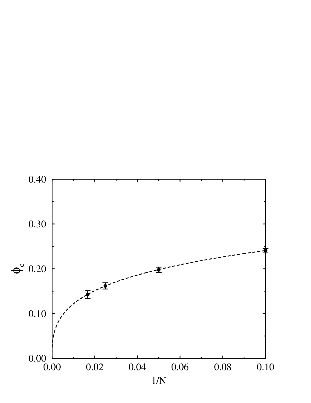
FIG. 7.: The measured estimates of the critical density as a function of chain length, together with the infinite $N$ value $\phi_{c}=0$ Also shown is a fit of the form $\phi_{c}=(1.1126+1.3N^{0.369})^{-1}$

FIG. 8.: The $N$ dependence of the end-to-end distance squared. The fit is of the form $R_{e}^{2}=5.653N^{1.112}$.

FIG. 9.: The measured function $p(R_{e}^{2})R_{e}^{-0.1245}$. Fits shows that $\nu>0.5$ implying that the chains are slightly swollen at criticality.

REFERENCES

- [1] P.J. Flory, Principles of Polymer Chemistry (Cornell univ. Press, Ithaca, N.Y., 1953), Ch. XIII.
- [2] H.E. Stanley, An Introduction to Phase Transitions and Critical Phenomena (Oxford University Press, Oxford, 1971).
- [3] B. Widom, Physica A194, 532 (1993).
- [4] S. Enders, B.A. Wolf and K. Binder, J. Chem. Phys. 103, 3809 (1995).
- [5] M.E. Fisher, Rev. Mod. Phys. 46, 597 (1974).
- [6] J.C. Le Guillou and J. Zinn-Justin, Phys. Rev. B21, 3976 (1980).
- [7] R. Perzynski, M. Delsanti and M. Adam, J. Phys. (Paris) 48 115 (1987).
- [8] T. Dobashi, M. Nakata and M. Kaneko, J. Chem. Phys. 72, 6685 (1980). ibid 6692 (1980).
- [9] K. Shinozaki, T.V. Tan, Y.Saito and T.Nose, Polymer 23 728 (1982).
- [10] I. C. Sanchez, J. Appl. Phys. 58, 2871 (1985).
- [11] B. Chu and Z. Wang, Macromolecules 21 2283 (1988).
- [12] I. C. Sanchez, J. Phys. Chem. 93, 6983 (1989).
- [13] K.-Q. Xia, C. Franck and B. Widom, J. Chem. Phys. 97 1446 (1992).
- [14] Y. Izumi and Y. Miyake, J. Chem. Phys. 1501 (1984) .
- [15] P.G. de Gennes, Scaling Concepts in Polymer Physics (Cornell Univ. Press, Ithaca, 1979) Ch. IV, §3.
- [16] M. Muthukumar, J. Chem. Phys. 85 4722 (1986).
- [17] S. Stepanow, J. Phys. (Paris) 48 2037 (1987).
- [18] A.L. Kholodenko and C. Qian, Phys. Rev. B40 2477 (1989).
- [19] B. J. Cherayil, J. Chem. Phys. 95, 2135 (1991); ibid 98, 9126 (1993).
- [20] D. Lhuillier, J. Phys. II (France) 2, 1411 (1992);ibid 3, 547 (1993).
- [21] V.I. Ginzburg, Soviet Phys-Solid State 2 1824 (1960).
- [22] K. Binder in Monte Carlo and Molecular Dynamics simulations in Polymer Science, K. Binder (ed.), Oxford University Press (1995).
- [23] B. Smit, S. Karaborni and J.I. Siepmann, J. Chem. Phys. 102, 2126 (1995).
- [24] Y-J. Sheng, A.Z. Panagiotopoulos, S.K. Kumar and I. Szleifer, Macromolecules 27, 400 (1994);
- [25] F.A. Escobedo and J.J. de Pablo, Mol. Phys. (in press).
- [26] A.Z. Panagiotopoulos, Fluid Phase Equilibria 76, 97 (1992); Mol. Simulation 9, 1 (1992).
- [27] A.D. Mackie, A.Z. Panagiotopoulos and S. K. Kumar, J. Chem. Phys. 102, 1014 (1995).
- [28] For a review, see V. Privman (ed.) Finite size scaling and numerical simulation of statistical systems (World Scientific, Singapore) (1990).
- [29] K. Binder in Computational Methods in Field Theory, H. Gausterer, C.B. Lang (eds.) Springer-Verlag Berlin-Heidelberg 59-125 (1992).
- [30] A. Sariban and K. Binder, J. Chem. Phys. 86 5859 (1987).
- [31] H.-P. Deutsch and K. Binder, Macromolecules 25 6214 (1992). H.-P. Deutsch and K. Binder, J. Stat. Phys. II (paris) 3, 1049 (1993). H.-P. Deutsch, J. Stat. Phys. 67 1039 (1992).
- [32] H.P. Deutsch, J. Chem. Phys. 99, 4825 (1993); M. Müller and K. Binder, Macromolecules, 28 1825 (1995); M. Müller and N.B. Wilding, Phys. Rev. E51 2079 (1995); M. Müller, Macromolecules 28, 6556 (1995).
- [33] A.M. Ferrenberg and R.H. Swendsen, Phys. Rev. Lett. 61 2635 (1988); ibid 63, 1195 (1989).
- [34] N.B. Wilding and A.D. Bruce, J. Phys. Condens. Matter 4, 3087 (1992); N.B. Wilding, Z. Phys. B93, 119 (1993); N.B. Wilding and M. Müller, J. Chem. Phys. 102, 2562 (1995).
- [35] I. Carmesin, K. Kremer, Macromolecules 21, 2819 (1988), H.P. Deutsch, K. Binder, J. Chem. Phys. 94, 2294 (1991), W. Paul, K. Binder, D.W. Heermann, and K. Kremer, J. Phys. II 1 37 (1991).
- [36] D. Frenkel, in Computer Simulation in Chemical Physics (M.P. Allen and D.J. Tildesley, eds.) Kluwer Acad. Publ. Dordrecht (1993).
- [37] J.I. Siepmann, Mol. Phys. 70, 1145 (1990).
- [38] D. Frenkel, G.C.A.M. Mooij and B. Smit, J. Phys. Condens. Matter 3, 3053 (1992).
- [39] R. Hilfer and N.B. Wilding, J. Phys. A28, L281 (1995).
- [40] B. Smit, Mol. Phys. 85 153 (1995).
- [41] C. Borgs and R. Kotecky, J. Stat. Phys 60, 79 (1990).
- [42] N.B. Wilding, Phys. Rev. E52 602 (1995),
- [43] P.-Y. Lai and K. Binder, J. Chem. Phys 97 586 (1992).
- [44] J. Des Cloizeaux and G. Jannick Polymers in solution (Oxford Univ. Press 1990).
- [45] Z. Alexandrowicz and N.B. Wilding, J. Chem. Phys. (in press)..
- [46] P. Biswas and B.J. Cherayil, J. Chem. Phys. 100, 4665 (1994).