Dynamical Mean Field Theory for Perovskites

Abstract

Using the Hubbard Hamiltonian for transition metal-3d and oxygen-2p states with perovskite geometry, we present a dynamical mean field theory which becomes exact in the limit of large coordination numbers or equivalently large spatial dimensions $D$. The theory is based on a new description of these systems for large $D$ using a selective treatment of different hopping processes which can not be generated by a unique scaling of the hopping element. The model is solved using a perturbational approach and an extended non-crossing approximation. We discuss the breakdown of the perturbation theory near half filling, the origin of the various 3d and 2p bands, the doping dependence of its spectral weight, and the evolution of quasi particles at the Fermi-level upon doping, leading to interesting insight into the dynamical character of the charge carriers near the metal insulator instability of transition metal oxide systems, three dimensional perovskites and other strongly correlated transition metal oxides.

I Introduction

The electronic structure of the strongly correlated copper oxide superconductors, other transition metal based perovskites, and of transition metal oxides like NiO, FeO or MnO has been an enduring problem in the last years [1, 2, 3, 4, 5, 6], still containing numerous unresolved questions. Among them are the nature of the insulating state, the evolution and doping dependence of coherent quasi particles near the Fermi energy in a doped Mott Hubbard or charge transfer insulator [7] and the transfer of spectral weight from high to low energy scales [8]. Experimentally, interesting variations of the spectroscopic and thermodynamic properties of these materials occur upon electron and hole doping [9, 10, 11, 12]. Recently, Tokura et al. [10] showed that Sr_1-xLa_xTiO₃ with perovskite-like structure exhibits a pronounced increase of the effective mass in approaching the insulating state while keeping the existence of a large Fermi surface which satisfies the Luttinger sum rule. They already argued that the different behavior of this compound compared to the pronounced two dimensional high-T_c cuprates might be due its three dimensional character. Furthermore, the transfer of spectral weight in Li-doped NiO  [11] and the investigation of hole and electron doping of this compound in Ref. [12] demonstrate the importance of strong electronic correlations in transition metal oxides. A systematic analysis of the electronic structure of 3d- transition metal compounds was recently performed by Saitoh et al. [6]. They showed that for a variety of materials like LaMnO₃, LaFeO₃, LaCoO₃, Mn_0.25TiS₂, Ni_0.33TiS₂, NiO, FeO, or MnO the character of the band gap is of the charge transfer type. Furthermore, the analysis of $x$-ray photoemission spectra [13] demonstrates the importance of the charge transfer mechanism in systems like V₂O₅, TiO₂ or LaCrO₃ and showed that many of the early transition metal compounds have to be reclassified as intermediate between the charge transfer and the Mott-Hubbard region or as falling into the charge transfer region itself. Consequently, it is of importance for an understanding of these materials that one takes the local spin and charge fluctuations of the transition metal and the oxygen states into account, i.e. both orbital degrees of freedom have to be described on the same footing.

For systems with one orbital degree of freedom a theoretical approach that allows the calculation of the excitation spectrum of strongly correlated systems, maintaining the dominating local correlations, was recently proposed by Metzner and Vollhard [14]. They introduced a dynamical mean field theory, where the system can be mapped on a local problem coupled to an effective bath. [15, 16, 17, 18] This dynamical mean field approach is exact in the limit of large coordination numbers or equivalently for large spatial dimensions ($D\rightarrow\infty$). [14, 19] In most applications of this approach, the one band Hubbard model is considered. A scaling of the hopping element like $t=t^{*}/\sqrt{D}$ with fixed $t^{*}$ leads for $D\rightarrow\infty$ to a remarkable simplification of the many body problem while retaining the nontrivial local dynamics of the elementary excitations and other main features of the model. [17, 18, 19, 20, 21, 22, 23]

Only few attempts have been made to extend the dynamical mean field theory to systems with more than one orbital degree of freedom. Valenti and Gros [24] realized that for the two band Hubbard model with perovskite structure, a scaling procedure similar to the one band model does not lead to a finite bandwidth. In order to avoid these difficulties Georges et al. [25] introduced a CuO model where two interpenetrating hypercubic lattices of copper and oxygen sites have been considered. This leads to a finite bandwidth and is able to describe interesting physics of the model under consideration. However, square root divergencies of the uncorrelated density of states occur, which result from the sublattice structure of the underlying lattice. This could limit the range of applicability of this model in the description of real transition metal oxides or possibly high-T_c systems.

In this paper we propose a scaling procedure to develop a reasonable model of perovskite systems for large $D$ based on a selective treatment of different hopping processes in large dimensions. It will be shown that this procedure leads to a large $D$ version of the three-band Hubbard model which reproduces important physics of the low dimensional situation. First, we solve this model using perturbation theory [17, 26] and show that this leads to a qualitatively wrong description of the physics near half filling. These problems are avoided by using an extended version of the non crossing approximation [27, 28, 29, 30, 31]. Finally, we discuss the doping dependence of the transition metal and oxygen densities of states. This is of interest due to the evolution of coherent quasiparticles near the Fermi energy, the transfer of spectral weight and the change of the effective mass upon doping.

II Theory

The dynamical mean field theory, which becomes exact in the limit of large coordination numbers, turned out to be a natural starting point for the description of highly correlated electronic systems like the one band Hubbard model and the Anderson lattice model. All this is based on a proper scaling of the hopping element, originally proposed in Ref. [14]. In the following, we show that the extension of this approach to more complex systems is only possible if one generalizes the idea of the scaling procedure in a way that the corresponding transfer functions between different unit cells, but not the hopping element itself, have to be scaled. This is demonstrated for the case of the two band Hubbard Hamiltonian, which describes hybridized transition metal (TM) and oxygen states with perovskite lattice structure. Similar to the one band case, the problem can be mapped onto an Anderson impurity problem and the enormous amount of theoretical tools, developed for the solution of this model, can be used. Furthermore, we show that the most natural choice of the corresponding impurity problem is to include all local orbitals into the impurity, not solely the strongly correlated ones. Otherwise, the set of self consistent equations is not well defined, leading to various computational problems. In our case, a cluster of hybridized TM- and O-sites is embedded into an effective medium. Physically, this is necessary because the charge and spin fluctuations of these two states are closely intertwined and have to be described on the same footing. The solution of the extended Anderson impurity model is performed using a perturbational approach [17, 26] and an extended version of the non crossing approximation [27, 28, 29, 30, 31]. The details of the latter method are presented in the appendix.

A Scaling procedure for large $D$

We consider the $D$-dimensional extension of the perovskite lattice, where the transition metal sites sit on a $D$-dimensional hypercubic lattice and the $D$ oxygen sites per unit cell are located between every two nearest neighbor TM sites. For simplicity, we consider only one TM 3d orbital. The corresponding ($D+1$)-band Hubbard Hamiltonian for the TM 3d and O 2p${}_{x_{\alpha}}$ ($\alpha=1,\ldots,D$) orbitals reads

$$H = \sum_{i,\sigma}\,\varepsilon_{d}d_{i\sigma}^{\dagger}d_{i\sigma}\,+\,\sum_{l,\sigma,\alpha}\,\varepsilon_{p}p_{l\sigma x_{\alpha}}^{\dagger}p_{l\sigma x_{\alpha}}\,$$ (2)

$$+\,t\sum_{il,\sigma,\alpha}\,g^{\alpha}_{il}(d_{i\sigma}^{\dagger}p_{l\sigma x_{\alpha}}\,+H.c.)+\,U\sum_{i}n_{i\uparrow}^{d}n_{i\downarrow}^{d}\,.$$

Here, $d_{i\sigma}^{\dagger}$ ($p_{l\sigma x_{\alpha}}^{\dagger}$) creates a hole in a TM-3d (O-2p${}_{x_{\alpha}}$ ) orbital at site $i$ ($l$) with spin $\sigma$. $\varepsilon_{d}$ and $\varepsilon_{p}$ are the corresponding on-site energies. $t$ is the amplitude of the nearest neighbor TM-O hopping integral and $U$ is the Coulomb repulsion between TM holes with occupation number operator $n_{i\sigma}^{d}=d_{i\sigma}^{\dagger}d_{i\sigma}$. The $p_{x_{\alpha}}-d$ hopping matrix elements have $pd\sigma$-symmetry, so that $g^{\alpha}_{il}=+1$ or $-1$ if $l=i+x_{\alpha}/2$ or $l=i-x_{\alpha}/2$, respectively. Only the combination $p_{{\rm s}i\sigma}=\frac{1}{\sqrt{2D}}\sum_{\l\alpha}\,g^{\alpha}_{il}p_{l\sigma x_{\alpha}}$ of oxygen states hybridizes with the d-states [32]. Since the operators $p_{{\rm s}i\sigma}$ do not anticommute, it is necessary to orthogonalize the corresponding states leading to $p_{{\bf k}\sigma}=\gamma_{\bf k}^{-1}p_{{\rm s}{\bf k}\sigma}$ where $p_{{\rm s}{\bf k}\sigma}$ is the Fourier transform of $p_{{\rm s}i\sigma}$ and

$$\gamma_{\bf k}^{2}=1-\frac{1}{D}\sum_{\alpha=1}^{D}\cos k_{\alpha}\,.$$ (3)

Besides the $p_{{\bf k}\sigma}$, which now fulfill standard fermion commutation relations, $D-1$ linear independent combinations of the Fourier transforms of $p_{l\sigma x_{\alpha}}^{\dagger}$ occur, which are orthogonal to $p^{\dagger}_{{\bf k}\sigma}$ and build up nonbonding oxygen orbitals. These nonbonding states at $\varepsilon_{p}$ decouple from the remainder of the system and do not have to be considered in the following calculation. The resulting Hamiltonian reads:

$$H = \sum_{{\bf k}\sigma}\left(\varepsilon_{d}d^{\dagger}_{{\bf k}\sigma}d_{{\bf k}\sigma}+\varepsilon_{p}p^{\dagger}_{{\bf k}\sigma}p_{{\bf k}\sigma}\right)$$ (5)

$$+\sqrt{2D}t\sum_{{\bf k}\sigma}\left(\gamma_{\bf k}d^{\dagger}_{{\bf k}\sigma}p_{{\bf k}\sigma}+H.c.\right)\,$$

This is a straightforward extension of the two band Hubbard model of perovskite systems to arbitrary dimension and can be used as the basis of a $1/D$ expansion. However, there exists no scaling of the form $t=t^{\ast}/D^{\beta}$ with exponent $\beta$ leading to a nontrivial limit for $D\rightarrow\infty$. Valenti and Gros [24] suggested a scaling with $\beta=1/2$ which leads to a zero bandwidth of the bonding and antibonding states, i.e. the TM-O ”dimers” of different lattice sites decouple. All other choices of $\beta$ lead either to zero or to infinite density of states.

In order to obtain a physically reasonable limit of the perovskites for large $D$ one has to bear in mind that different hopping processes which are of the same order in $t$ are of different importance for large $D$. Due to the local character of the Coulomb interaction, it is sufficient to perform the scaling at first for $U=0$. For the calculation of the single particle Green’s function one has to sum up all closed paths on the lattice under consideration. In Fig. 1 we show two different hopping processes which are of forth order in $t$. There are $4D^{2}$ processes of type (a) and only $2D$ processes of type (b). Using a scaling like $t=t^{\ast}/\sqrt{D}$ the contribution of the (a) processes to the Green’s function are of order $1$ whereas the (b) processes have only contributions of order $1/D$ and are suppressed for $D\rightarrow\infty$ leading to the zero bandwidth of Ref. [24]. This results from the TM coordination number being $2D$ whereas the oxygen coordination number is $2$. A selective consideration of these different paths can be obtained by the following partial summation of paths starting at TM-site $i$ and ending at the TM-site $j$:

$$G^{o}_{d\,ij}(\omega)=G^{at}_{d}(\omega)\delta_{ij}+G^{at}_{d}(\omega)T_{ij}(\omega)G^{at}_{d}(\omega)$$ (6)

$$+\sum_{l}\,G^{at}_{d}(\omega)T_{il}(\omega)G^{at}_{d}(\omega)T_{lj}(\omega)G^{at}_{d}(\omega)\,\,\,+\cdots\,\,\,.$$ (7)

Here, the local d-Green’s function

$$G^{at}_{d}(\omega)=\left(\omega-\varepsilon_{d}-\frac{2Dt^{2}}{\omega-\varepsilon_{p}}\right)^{-1}$$ (8)

contains all TM-O-TM hopping processes, where the path returns to the starting TM-site without entering any other TM site ((a) processes). The transfer function $T_{ij}(\omega)$ which is given by $(-t^{2})/(\omega-\varepsilon_{p})$ for neighboring TM sites and zero otherwise has the character of an effective, but frequency dependent TM-TM hopping element $T_{ij}\propto\delta_{\langle ij\rangle}t^{2}$ ((b) processes). Therefore, we propose the following scaling procedure, where the two different hopping processes are treated differently:

$$G^{at}_{d}(\omega)=\left(\omega-\varepsilon_{d}-\frac{4(t^{*})^{2}}{\omega-\varepsilon_{p}}\right)^{-1}\,\,;\,\,\,\,\,\,\,t^{*}=\sqrt{D/2}t\,,$$ (9)

$$T_{ij}(\omega)=-\delta_{\langle ij\rangle}\sqrt{\frac{2}{D}}\frac{(t^{*})^{2}}{\omega-\varepsilon_{p}}\,\,;\,\,\,\,\,\,\,\,\,(t^{*})^{2}=\sqrt{D/2}t^{2}\,.$$ (10)

Here, the effective TM-TM hopping $T_{ij}$ (not $t$ itself) has been scaled in analogy to the one band case. Consequently, the processes of Fig. 1b are no more suppressed relative to that of Fig. 1a. The summation of all closed paths on the remaining hypercubic TM-lattice is straightforward and leads to the d-Green’s function for $U=0$:

$$G^{o}_{d}(\omega)=\frac{\omega-\varepsilon_{p}}{4(t^{*})^{2}}\int dy\frac{\varrho_{o}(y-1)}{(\omega-\varepsilon_{p})(\omega-\varepsilon_{d})/4(t^{*})^{2}-y}\,,$$ (11)

where the reduced density of states $\varrho_{o}(y)$ is defined by

$$\varrho_{o}(y)=\frac{1}{N}\sum_{\bf k}\,\delta\left(y-\frac{1}{\sqrt{2D}}\alpha_{\bf k}\right)\,,$$ (12)

with $\alpha_{\bf k}=\sum_{\nu=1}^{D}{\rm cos}k_{\nu}$. The oxygen Green’s function $G^{o}_{p}(\omega)$ which refers to the states $p_{{\bf k}\sigma}$ can be obtained from $G^{o}_{d}(\omega)$ by interchanging $\varepsilon_{d}$ and $\varepsilon_{p}$. The large $D$ behavior of $\varrho_{o}(y)$ is, in analogy to the one band case, given by a Gaussian distribution function $\sqrt{2/\pi}\exp(-2y^{2})$. [19] For simplicity, we use in the following a semi elliptical reduced density of states $\varrho_{o}(y)=2/\pi\sqrt{1-y^{2}}$ if $y^{2}<1$ and zero otherwise. This Bethe lattice of the TM-sites does not changes the relative local arrangement of TM and O sites, typical for perovskite systems. Finally, it is interesting to point out, that this selected treatment of different hopping processes can be generated by the Hamiltonian of Eq. 5, if one performs the following scaling transformation of the coherence factor:

$$t^{2}D\gamma_{\bf k}^{2}\rightarrow 2(t^{*})^{2}-2\sqrt{\frac{2}{D}}(t^{*})^{2}\alpha_{\bf k}\,.$$ (13)

Based on this formulation of the large $D$ version of the TM-O system for $U=0$, it is straightforward to show for $U\neq 0$, in analogy to the one band case, that the self energy $\Sigma_{d}(\omega)$ of TM-holes is momentum independent. Consequently, one finds for the TM-Green’s function within the Bethe lattice:

$$G_{d}(\omega)^{-1} =\omega-\varepsilon_{d}-\Sigma_{d}(\omega)-\frac{4t^{2}}{\omega-\varepsilon_{p}}$$ (15)

$$-\frac{1}{4}\left(\frac{4t^{2}}{\omega-\varepsilon_{p}}\right)^{2}G_{d}(\omega).$$

This results from the representation of the Green’s function with semi-elliptical density of states:

$$G_{d}(\omega) = \frac{1}{N}\sum_{\bf k}G_{d}({\bf k},\omega)$$ (17)

$$=\frac{\omega-\varepsilon_{p}}{4t^{2}}{\cal F}\left(\frac{(\omega-\varepsilon_{p})(\omega-\varepsilon_{d}-\Sigma_{d}(\omega))}{4t^{2}}\right),$$

with ${\cal F}(z)\equiv 2\left(z-1-\sqrt{(z-1)^{2}-1}\right)$ and the relation ${\cal F}(z)^{-1}=z-1-\frac{1}{4}{\cal F}(z)$. Furthermore, the system can be mapped onto an Anderson model with effective hybridization and additional self consistency condition.

Finally, we note that the additional consideration of the TM-O Coulomb repulsion $U_{pd}$ would lead to further frequency dependent contributions of the self energies $\Sigma_{\alpha\beta}(\omega)$ ($\alpha\beta\in\{p,d\}$). This results from the small coordination number of the oxygen sites and is different in the one band case, where each intersite Coulomb repulsion contributes in zeroth order of $1/D$ only through its Hartree-Fock value [19]. Therefore, the limit $D\rightarrow\infty$ might be an interesting approach for a detailed consideration of the dynamical interplay of spin and charge fluctuations of transition metal oxides.

B Effective TM-O impurity model

As in the one band case, the large-D version of a TM-O model is mapped onto an effective impurity model. Due to the occurrence of an additional orbital degree of freedom, the choice of the corresponding effective medium is not unique. Although, the most obvious choice might be to embed only the TM-site into an effective medium and to change solely the self consistence condition, it is straightforward to show that this leads to a divergence of the hybridization of this medium at the oxygen on-site energy $\varepsilon_{p}$. This is due to the fact that the effective medium has to simulate not solely the correlated TM-sites but also the existence of the oxygen states. In order to avoid this divergency, we propose in the following an impurity model where a cluster of one TM- and one O-orbital is embedded within an effective medium. This is illustrated in Fig. 2. Motivated by the perovskite geometry, we couple the effective medium only to the oxygen sites. Furthermore, the local TM-O hybridization within the cluster is explicitly taken into account. This leads to a well defined effective medium. The corresponding Hamiltonian reads:

$$H_{\rm eff}=H_{\rm loc}+H_{\rm med}\,,$$ (18)

where the local part is given by

$$H_{\rm loc}=\sum_{\sigma}\left(\varepsilon_{d}n_{\sigma}^{d}+\varepsilon_{p}n_{\sigma}^{p}+2t\left(d_{\sigma}^{\dagger}p_{\sigma}+p_{\sigma}^{\dagger}d_{\sigma}\right)\right)+Un_{\uparrow}^{d}n_{\downarrow}^{d}$$ (19)

and

$$H_{\rm med}=\sum_{{\bf{k}}\sigma}\left(W_{\bf{k}}c_{{\bf{k}}\sigma}^{\dagger}p_{\sigma}+H.c.\right)+\sum_{{\bf{k}}\sigma}\varepsilon_{\bf{k}}c_{{\bf{k}}\sigma}^{\dagger}c_{{\bf{k}}\sigma}$$ (20)

describes the coupling of the oxygen states with the effective medium, characterized by the hybridization

$${\cal J}(\omega)=\sum_{\bf{k}}\frac{|W_{\bf{k}}|^{2}}{\omega+i0^{+}-\varepsilon_{\bf{k}}}\,.$$ (21)

This coupling of the effective medium to the oxygen states, although not unique, is physically motivated by the local arrangement of the original lattice. From the equation of motion of the effective Hamiltonian, it follows

$$G_{d}(\omega)^{-1}=\omega-\varepsilon_{d}-\Sigma_{d}(\omega)-\frac{4t^{2}}{\omega-\varepsilon_{p}-{\cal J}(\omega)}\,.$$ (22)

Comparing this with Eq. 15, one immediately finds:

$${\cal J}(\omega)=t^{2}G_{d}(\omega)\left(1-\frac{t^{2}G_{d}(\omega)}{\omega-\varepsilon_{p}-t^{2}G_{d}(\omega)}\right)\,.$$ (23)

This is the self-consistant equation of the theory, based on the condition that the Green’s function of the impurity model defined in Eq. 18 equals that of the lattice system. Note that this effective medium, which represents the states coupled to the oxygen, is predominantly determined by the correlated TM-sites.

In the following we solve the impurity model of Eq. 18 using the iterated perturbation theory (IPT), and an extended version of the non crossing approximation (NCA), where the effective medium is fixed by Eq. 23. Since it was necessary for the consideration of the TM-O cluster to generalize the standard NCA-scheme to more local eigenstates, the corresponding details are given in the appendix.

III Results

In the following, we present our results for the TM- and O-densities of states obtained within the IPT and NCA. In Fig.  3 we show our results for the TM- and O-densities of states obtained within the IPT for half filling $x=0$ ($x=n_{d}+n_{p}-1$). Two Hubbards bands which are dominated by TM-states are separated by $U$ and two oxygen dominated bands in the neighborhood of $\varepsilon_{p}$ are visible. Similar to the one band case, the IPT leads to an interesting structure of the density of states, where now four bands are occurring. However, the expected insulating behavior at half filling (for large $U$) does not occur. This results from the overestimation of the spectral weight of the lower Hubbard band within the IPT by $\propto 1-n_{d}$. The occupation of oxygen sites ($n_{p}>0$) due to TM-O hybridization leads to an overcounting of copper sites which can be occupied without paying any Coulomb energy. Therefore, the success of the IPT in the one band case [17] does not occur within the two band model. This is due to the absence of the particle-hole symmetry and the change of the TM-occupation number $n_{d}$ as function of $t$ at half filling. This shortcoming of the IPT results from the occupation of O sites and is expected to vanish for small $n_{p}$ which occurs in the limit of a large value for $\Delta=\varepsilon_{p}-\varepsilon_{d}$. However, for the physically interesting situation $\Delta\approx U/2$, the IPT leads to qualitatively wrong results and one has to develop theoretical approaches which take the local TM-O many body states explicitly into account. Therefore, we use the NCA , which was shown to be in excellent agreement with quantum Monte Carlo (QMC) simulations in the one band case, such that a local TM-O hybrid with 16 local eigenstates is coupled to an effective medium. Here, the TM-O singlet state which is related to an important excitation near half filling is explicitly taken into account.

In Fig.  4 we show the TM- and O-densities of states at half filling and for a hole and an electron doped system, obtained within the non crossing approximation. The calculations are performed for $U=2\Delta=10t$ and $t=1\,{\rm eV}$. At half filling we find now the expected insulating state, i.e. the Fermi level lies in the middle of the charge transfer gap. In this charge transfer regime we find bands dominated by TM-states (B, F, and G) which are separated by the Coulomb repulsion $U$ due to the Mott-Hubbard splitting and on both sides of the charge transfer gap TM- and O-dominated bands (B and C). Besides the O-dominated band above the charge transfer gap (C-D) a second one for higher excitation energy occurs (E). A detailed analysis of the transitions between the various many body states of the local TM-O hybrid reveals that these are build up by the TM-O singlet and triplet states. All these features of the density of states are believed to be general properties of the model under consideration [33] and are also qualitatively in agreement with exact cluster diagonalizations and Monte Carlo simulations for two dimensional systems. [34, 35, 36] This demonstrates that it is indeed possible to reproduce important physical phenomena of the low dimensional situation within the large $D$ approach. Besides this general structure on a larger energy scale, a coherent quasi particle peak near the Fermi level occurs, which shows up an interesting temperature and doping dependency (see below).

In order to clarify the origin of the details of the density of states, we investigated which transitions between the local many body states are predominately responsible for each band. Technically, this is performed within the NCA if one restricts the available Hilbert space according to the general scheme presented in the appendix. If the spectral weight of a band decreases after projecting out a certain local state $|m\rangle$, a transition from or into this state is responsible for the band. This analysis is of particular importance, if one is interested in calculations within a restricted Hilbert space of the most important states. The results are presented in Fig. 4b for hole doped systems, whereby the meaning of the state labels are given in Tab. I. The leading contribution is underlined while negligible contributions are embraced.

The main contributions to the bands B and E occur also for an uncorrelated system and are build up by transitions between an empty state $|0\rangle$ and a bonding ($|d_{\sigma}\rangle$) or antibonding ($|p_{\sigma}\rangle$) combination of TM- and O-states, respectively. More interesting are the bands A, C, F, and G, because they are purely due to strong electronic correlations. Here, the bands F and G are due to transitions from the TM-dominated state $|d_{\sigma}\rangle$ to states which are dominated by doubly occupied TM sites, i.e. they form the upper Hubbard band. Band C contains essentially the well known TM-O Zhang Rice singlet state [32] resulting from a transition from the bonding state $|d_{\sigma}\rangle$ to the state $|S_{o}\rangle$ dominated by the TM-O singlet state. other contributions close in energy are identified under label D. Furthermore, a pronounced part of band E, which consists predominantly of antibonding $|p_{\sigma}\rangle$ states, results also from the transition of singly occupied sites to TM-O triplet states $|T_{\pm}\rangle$ . Consequently, we find a singlet triplet splitting which compares well with the result $8J$ obtained from perturbation theory in $t$ for two spatial dimensions, where $J=t^{2}(\Delta^{-1}+(U-\Delta)^{-1})$. [37] Finally, the lowest state A results from a transition between the antibonding state $|p_{\sigma}\rangle$ and the singlet state $|S_{o}\rangle$. Interestingly, this state occurs for very low excitation energies and only in systems with an occupied singlet state, i.e. for hole doped systems. This is a consequence of the fact that the singlet state with two particles per TM-O unit has lower energy than the singly occupied antibonding state $|p_{\sigma}\rangle$.

This interpretation of the various bands in terms of the transitions between many body states allows a transparent explanation of the doping dependence of their spectral weight. In Fig. 5 we show the spectral weight of various bands upon electron and hole doping. For hole doping we plot in part a of the figure the spectral weight of all occupied states and of the occupied part of the singlet band (low energy hole states). The latter demonstrates that the transfer of spectral weight, discussed in Ref. [8], is included within our approach. As expected, the spectral weight of the bonding band decreases upon doping. However, band A which results from the transition between $|S_{o}\rangle$ and $|p_{\sigma}\rangle$ increases, because upon hole doping more initial singlet states are available The corresponding result for the electron doped materials are shown in Fig. 5b, where we plot the spectral weight of all unoccupied bands and that of the unoccupied part of the lower Hubbard band B which carries the Fermi level (low energy electron states). While the spectral weight of the bands which are purely due to correlations decreases, band E increases upon electron doping. The character of the system becomes much more uncorrelated leading to an increase of the bonding and antibonding TM-O states which are present also for $U=0$ with even larger spectral weight.

Based on this analysis, which demonstrates that the density of states near the Fermi level is build up by the transitions between only a few local many body states, it is interesting to perform the calculation within a restricted Hilbert space. In Fig. 6 we show the TM- and O-densities of states if one takes only the states $|0\rangle$, $|p_{\sigma}\rangle$,$|d_{\sigma}\rangle$,$|S_{o}\rangle$, and $|T_{\pm}\rangle$ into account. The results are compared with that for the full Hilbert space (dashed line). It is impressive, that the details of the single particle excitation spectrum near the Fermi level are very well reproduced by this restricted set of states. Note that this calculation includes still the full information about the orbital character of the low energy spectrum. This might be of interest for the theoretical description of more complex systems where the diagonalization of the local problem leads to extremely large numbers of coupled integral equations of the NCA. The most important states can straightforwardly be found from the eigenstates of the complete local problem, since the peak position is well reproduced from the corresponding difference of the relative eigenenergies, as given in Tab. I.

Finally, we present our results for the coherent low energy peak near the Fermi level. In Fig. 7 we show the density of states near the Fermi level ($\omega=0$) for a hole doping concentration $x=0.2$ for various temperatures [38]. For electron doping, the corresponding low energy part of the spectrum behaves very similarly. Although the density of states at the Fermi level is almost constant, the states near the Fermi energy are strongly temperature dependent. For decreasing temperature, a coherent quasi particle peak occurs which builds up its maximum slightly below the Fermi energy.

In Fig. 8a and b we present our results for the doping dependence of the low energy part of the spectrum for a hole doped system in the charge transfer and for an electron doped system in the Mott-Hubbard regime at $T=300\,{\rm K}$. As expected, the general behavior of the low energy part of the total density of states is relatively similar in both regimes. The evolution of these quasiparticles results in a large effective mass ratio obtained via $m^{*}/m=\left.(1-\partial{\rm Re}\Sigma_{d}(\omega)/\partial\omega)\right|_{\omega=0}$. In Fig. 8c, as a representive example we show results for a electron doped material in the charge transfer regime. This shows clearly the mass enhancement when approaching the insulating regime either charge transfer or Mott Hubbard type and resembles the doping dependence of the effective mass obtained within the Brinkmann-Rice transition [43, 44], where only the coherent part of the spectrum occurs. In addition, we plot in part a of Fig. 8 the density of states for low hole doping ($x=0.017$) but for large temperatures of $T=1000\,{\rm K}$. This shows that the quasi particle peak disappears completely between $300$ and $1000\,{\rm K}$, giving rise to an enormous temperature dependence of the low energy excitations in slightly doped perovskite systems. The enhancement of $m^{*}/m$ with band filling agrees with the observed behavior in Sr_1-xLa_xTiO₃ [10] which is believed to fall into the the Mott-Hubbard regime. Furthermore, the measurement of the Hall coefficient indicates the formation of a large Fermi surface. Although our dynamical mean field approach does not allow an investigation of the momentum dependent spectral density

$\displaystyle A({\bf k},\omega)\approx\frac{m}{m^{*}}\delta(\omega-\varepsilon^{*}_{\bf k})+A^{\rm incoh.}({\bf k},\omega)\,,$

we believe that a large effective mass ratio $m^{*}/m$ leads to a large Fermi surface formed by the coherent part of the spectrum $\frac{m}{m^{*}}\delta(\omega-\varepsilon^{*}_{\bf k})$ with renormalized quasi particle energy $\varepsilon^{*}_{\bf k}$. This is possible because only a few particles can occupy a large number of momentum states due to its low spectral weight $\frac{m}{m^{*}}$. The physical origin of the coherent quasiparticle resonance is similar to the conventional Abrikosov-Suhl resonance of systems with magnetic impurities. In the charge transfer regime, for hole doping, the resonant transition between a bonding state $|d_{\sigma}\rangle$ and the Zhang Rice singlet $|S_{o}\rangle$ builds up the Kondo like peak. For electron doping, it is correspondingly a transition between an empty state $|0\rangle$ and $|d_{\sigma}\rangle$.

IV Conclusions

In conclusion, we presented a dynamical mean field theory for perovskites which is based on a new scaling procedure of the large dimensional Hubbard model of transition metal 3d and oxygen 2p states. In the limit $D\rightarrow\infty$, the electronic self energy is, similar to the one band case, momentum independent and the model can be mapped onto an Anderson impurity model. It is demonstrated that the most natural choice of this impurity is to include all local orbitals of one unit cell, not solely the strongly correlated ones. Correspondingly a model with 16 local many body states is embedded into an effective medium which has to be determined self consistently. Motivated by the perovskite lattice geometry, this effective medium is coupled only to the oxygen sites of the impurity and simulates predominantly the TM-sites of the real lattice. The solution of the local problem is performed using the iterated perturbation theory and an extended noncrossing approximation. Is is shown that the spectral weight of the various bands of the density of states is erroneously described within the IPT. This shortcoming results from the missing electron hole symmetry of the half filled model, leading to an absence of a metal insulator transition for half filling. In distinction, the NCA is able to describe this problem properly and gives interesting insight into the origin and doping dependence of the various bands of the TM- and O-densities of states. Furthermore, the occurrence and doping as well as temperature dependencies of a coherent quasi particle peak near the Fermi level is discussed. This results from a Kondo like resonance between an empty and a bonding TM-O state for electron doping and this bonding state and the Zhang Rice singlet state for hole doping. Finally, it is shown that the restriction of the local states to a limited set of most important states reproduces very well the low energy density of states, keeping the full orbital information of the involved states. This is of importance for an extension of the theory to more realistic situations including all five d-bands such that only a small number of coupled NCA equations have to be solved. This might be stimulating for further theoretical studies of transition metal compounds within the dynamical mean field approach.

A Non Crossing Approximation of a TM-O Cluster

In this appendix, we discuss an extended version of the non crossing approximation for an impurity model given in Eq. 18. The NCA was shown to be in excellent agreement with quantum Monte-Carlo calculations for the dynamical mean-field theory of the one band case [22, 23]. This approximation is not a perturbational expansion with respect to the Coulomb repulsion U, but takes into account all eigenstates of the local part of the impurity Hamiltonian, by performing an expansion with respect to the hybridization ${\cal J}(\omega)$. Therefore, we rewrite the Hamiltonian of Eq. 18 in terms of the Hubbard operators $X_{m^{\prime}m}\equiv|m^{\prime}\rangle\langle m|$, where $|m\rangle$ is, in our case, one of the 16 eigenstates of $H_{loc}$, with eigenvalue $E_{m}$ (see Tab. I):

$$H_{loc} = \sum_{\sigma m}E_{m}X_{mm}\,,$$

$$H_{med} = \sum_{{\bf{k}}\sigma mm^{\prime}}\left(W_{\bf{k}}c_{{\bf{k}}\sigma}^{\dagger}P_{mm^{\prime}}^{\sigma}X_{mm^{\prime}}+H.c.\right)+\sum_{{\bf{k}}\sigma}\varepsilon_{\bf{k}}c^{\dagger}_{{\bf{k}}\sigma}c_{{\bf{k}}\sigma}\,.$$

The eigenvalues of $H_{loc}$ are explicitly given in Ref. [42]. The $(16\times 16)$ matrix $P^{\sigma}$ and a corresponding matrix $D^{\sigma}$ are defined by the following representation of the O- and TM-destruction operators:

$$p_{\sigma} = \sum_{m,m^{\prime}}P_{mm^{\prime}}^{\sigma}X_{mm^{\prime}}\,,$$

$$d_{\sigma} = \sum_{m,m^{\prime}}D_{mm^{\prime}}^{\sigma}X_{mm^{\prime}}\,.$$

Using this representation of the Hamiltonian, one introduces within NCA scheme the local propagators for each of the eigenstates $|m\rangle$:

$$P_{m}(\omega)=\frac{1}{\omega+i0^{+}-E_{m}-\Sigma_{m}(\omega)}\,,$$ (A1)

with the corresponding spectral density $p_{m}(\omega)=-\frac{1}{\pi}~{}{\rm Im}P_{m}(\omega+i0^{+})$. The NCA self energies are given by:

$$\Sigma_{m}(\omega) = -\frac{1}{\pi}\sum_{\sigma,m^{\prime}}|P_{m,m^{\prime}}^{\sigma}|^{2}\int_{-\infty}^{+\infty}d\varepsilon f\left(\eta_{m,m^{\prime}}\varepsilon\right)$$ (A3)

$${\rm Im}{\cal J}(\varepsilon+i0^{+})P_{m^{\prime}}\left(\omega+\eta_{m,m^{\prime}}\varepsilon\right)\,.$$

Here, $f(\varepsilon)$ is the Fermi distribution function and $\eta_{m,m^{\prime}}=+1$ (resp. $-1$) if the particle number of the state $|m^{\prime}\rangle$ is higher (resp. lower) than the particle number of the state $|m\rangle$. In Eq. A3, we neglect the vertex corrections discussed in Refs. [31, 39, 40, 41]. Although this was shown to slightly underestimate the Kondo temperature and to shift the Abrikosov-Suhl resonance slightly away from the chemical potential, it gives important insights into the low energy excitations, in particular for large values of the Coulomb repulsion. Furthermore, in view of the enormous numerical problems, which arizes if one calculates these vertex corrections even for less complex systems than ours, [40, 41] and due to the additional self consistent condition of the large $D$ approach, it is actually very difficult to go beyond Eq. A3. Finally, the Green’s functions of the system, which give the information about the single particle excitation spectrum, result from:

$$G_{d}(\omega) = \sum_{m,m^{\prime}}|D_{mm^{\prime}}^{\sigma}|^{2}\langle\langle X_{m^{\prime}m};X_{mm^{\prime}}\rangle\rangle_{\omega}\,,$$ (A4)

$$G_{p}(\omega) = \sum_{m,m^{\prime}}|P_{mm^{\prime}}^{\sigma}|^{2}\langle\langle X_{m^{\prime}m};X_{mm^{\prime}}\rangle\rangle_{\omega}\,,$$ (A5)

where $\langle\langle X_{m^{\prime}m};X_{mm^{\prime}}\rangle\rangle_{\omega}$ is the Fourier transform of the retarded Green’s function $-i\theta(t)\langle[X_{m^{\prime}m}(t);X_{mm^{\prime}}(0)]_{+}\rangle$. They can be expressed with respect to the NCA local propagators as following:

$$\langle\langle X_{m^{\prime}m};X_{mm^{\prime}}\rangle\rangle_{\omega} = \frac{1}{Z_{0}}\int_{-\infty}^{\infty}d\varepsilon{e}^{-\beta\varepsilon}\left(p_{m^{\prime}}(\varepsilon)P_{m}(\omega+\varepsilon)\right.$$ (A7)

$$\left.-p_{m}(\varepsilon)P_{m^{\prime}}(\omega-\varepsilon)^{*}\right)\,,$$

where the partition sum $Z_{0}$ is defined by $\sum_{m}\int_{-\infty}^{\infty}d\varepsilon{e}^{-\beta\varepsilon}p_{m}(\varepsilon)$. All the summations with respect to $m$ and $m^{\prime}$ are performed over the 16 eigenstates of $H_{loc}$. As can be seen from Tab. I the spin degeneracy leads to only 11 different eigenstates and propagators in the paramagnetic state. The solution of Eq. A1 and A3, which are coupled singular integral equations, is performed using the fast Fourier transformation for the convolution integrals and using the defect propagators of the local eigenstates [28, 29].

state label	state	degeneracy	occupation $n_{o}$	$E_{m}-\mu n_{o}$
1	$|0\rangle$	1	0	0
2	$|d_{\sigma}\rangle=(\cos\phi d^{\dagger}_{\sigma}+\sin\phi p^{\dagger}_{\sigma})|0\rangle$	2	1	-0.701
3	$|p_{\sigma}\rangle=(\cos\phi d^{\dagger}_{\sigma}-\sin\phi p^{\dagger}_{\sigma})|0\rangle$	2	1	5.701
4	$|T_{o}\rangle=\frac{1}{\sqrt{2}}(d^{\dagger}_{\uparrow}p^{\dagger}_{\downarrow}+d^{\dagger}_{\downarrow}p^{\dagger}_{\uparrow})|0\rangle$	1	2	5
5	$|T_{\sigma}\rangle=d^{\dagger}_{\sigma}p^{\dagger}_{\sigma}|0\rangle$	2	2	5
6	$|S_{o}\rangle=[u_{1}d^{\dagger}_{\uparrow}d^{\dagger}_{\downarrow}+v_{1}p^{\dagger}_{\uparrow}p^{\dagger}_{\downarrow}$	1	2	2.738
	$\ \ \ \ \ \ \ -w_{1}(d^{\dagger}_{\uparrow}p^{\dagger}_{\downarrow}-d^{\dagger}_{\downarrow}p^{\dagger}_{\uparrow})]|0\rangle$
7	$|dd\rangle=[u_{2}d^{\dagger}_{\uparrow}d^{\dagger}_{\downarrow}+v_{2}p^{\dagger}_{\uparrow}p^{\dagger}_{\downarrow}$	1	2	12.217
	$\ \ \ \ \ \ \ -w_{2}(d^{\dagger}_{\uparrow}p^{\dagger}_{\downarrow}-d^{\dagger}_{\downarrow}p^{\dagger}_{\uparrow})]|0\rangle$
8	$|pp\rangle=[u_{3}d^{\dagger}_{\uparrow}d^{\dagger}_{\downarrow}+v_{3}p^{\dagger}_{\uparrow}p^{\dagger}_{\downarrow}$	1	2	10
	$\ \ \ \ \ \ \ -w_{3}(d^{\dagger}_{\uparrow}p^{\dagger}_{\downarrow}-d^{\dagger}_{\downarrow}p^{\dagger}_{\uparrow})]|0\rangle$
9	$|D_{\sigma}\rangle=(\cos\theta d^{\dagger}_{\sigma}p^{\dagger}_{\sigma}d^{\dagger}_{-\sigma}$
	$\ \ \ \ \ \ \ +\sin\theta d^{\dagger}_{\sigma}p^{\dagger}_{\sigma}p^{\dagger}_{-\sigma})|0\rangle$	2	3	9.298
10	$|P_{\sigma}\rangle=(\cos\theta d^{\dagger}_{\sigma}p^{\dagger}_{\sigma}p^{\dagger}_{-\sigma}$
	$\ \ \ \ \ \ \ -\sin\theta d^{\dagger}_{\sigma}p^{\dagger}_{\sigma}d^{\dagger}_{-\sigma})|0\rangle$	2	3	15.702
11	$|DP\rangle=d^{\dagger}_{\uparrow}p^{\dagger}_{\uparrow}d^{\dagger}_{\downarrow}p^{\dagger}_{\downarrow}|0\rangle$	1	4	20

TABLE I.: The degeneracy, occupation and relative energy of all local eigenstates introduced in the appendix and the corresponding labels used in Fig. 4 are given. The eigenvalues are obtained for $U=10\,{\rm eV}$, $\Delta=5\,{\rm eV}$, and $t=1\,{\rm eV}$. Here, $\tan 2\phi=-\frac{4t}{\Delta}$ and $\tan 2\theta=\frac{4t}{\Delta+U}$ . The coefficients $u_{i}$, $v_{i}$, and $w_{i}$ can be obtained from the diagonalization of the three dimensional space build up by $|S_{o}\rangle$, $|dd\rangle$, and $|pp\rangle$, see for example Ref. [42].

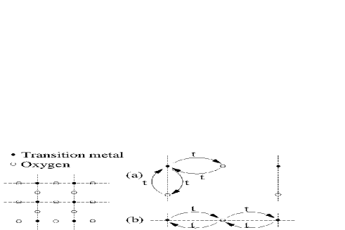
FIG. 1.: Hopping processes of order $t^{4}$ which are of different importance for large $D$. Since there are $4D^{2}$ processes of type (a) but only $2D$ processes of type (b), the latter are suppressed compared to the former for large dimensions.

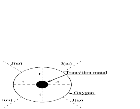
FIG. 2.: Schematic impurity model where a cluster of one TM- and O-site is embedded within an effective medium. Here, the local hybridization $t$ between the two local sites is explicitly taken into account. The effective medium is coupled only to the oxygen states.

      

FIG. 3.: TM (solid line) and O (dashed line) density of states obtained within the iterated perturbation theory for half filling. Note that the spectral weight of the various bands is erroneously described within the IPT such that no insulator occurs for half filling.

      

FIG. 4.: TM (solid line) and O (dashed line) density of states obtained within the hybrid-NCA at half filling (a) for hole doping $x=0.1$ (b) and electron doping $x=-0.1$ (c). For hole doping it is indicated which transitions between the local states contribute to the corresponding bands, where the meaning of the state labels is given in Tab. 1. The leading contribution is underlined while negligible contributions are embraced.

FIG. 5.: Doping dependence of the spectral weight multiplied with the spin degeneration of the occupied bands and the occupied part of the singlet band (low energy hole states) for hole doping (a) and of the unoccupied bands and the unoccupied part of the lower Hubbard band (low energy electron states) for electron doping (b).

FIG. 6.: TM (a) and O (b) density of states obtained within the hybrid-NCA for hole doping $x=0.1$ within a restricted Hilbert space of the local states $|0\rangle$, $|d_{\sigma}\rangle$, $|p_{\sigma}\rangle$, $|T_{\sigma}\rangle$, and $|S_{o}\rangle$ in comparison with the results of the full local space (dashed lines).

FIG. 7.: Density of states near the Fermi level for hole doping $x=0.2$ and for various temperatures. Note the formation of a coherent quasi particle peak resulting from Kondo like resonances between the singly occupied bonding TM-O state and the doubly occupied singlet state.

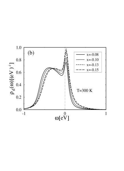
FIG. 8.: Doping dependence of the coherent quasi particle peak for $T=300\,{\rm K}$ in the charge transfer regime with $U=10\,{\rm eV}$, $\Delta=5\,{\rm eV}$ (a) and in the Mott-Hubbard regime with $U=5\,{\rm eV}$, $\Delta=9.5\,{\rm eV}$ (b). In both cases we use $t=1\,{\rm eV}$. The effective mass in the charge transfer regime and for electron doping is shown in part (c). For comparison we also plot in the inset the result for low hole doping ($x=0.017$) but high temperature $T=1000\,{\rm K}$ which demonstrates that strong temperature dependence occurs in the low doping regime.

REFERENCES

- [1] J. G. Bednorz and K. A. Müller, Z. Phys. B 64, 189 (1986).
- [2] Y. Fujishima, Y. Tokura, T. Arima, and S. Uchida, Physica C 185, 1001 (1991).
- [3] T. Arima, Y. Tokura, and J. B. Torrance, Phys. Rev. B 48, 17006 (1993).
- [4] S. Hüfner, Advances in Physics 43, 183 (1995).
- [5] Z.-X. Shen and D. S. Dessau, Physics Rep. 253, 1 (1995).
- [6] T. Saitoh, A. E. Bocquet, T. Mizokawa, and A. Fujimori, Phys. Rev. B 52, 7934 (1995).
- [7] J. Zaanen, G. A. Sawatzky, and J. A. Allen, Phys. Rev. Lett. 55, 418 (1985).
- [8] H. Eskes, M. B. J. Meinders, and G. A. Sawatzky, Phys. Rev. Lett. 67, 1035 (1991).
- [9] S. A. Carter, T. F. Rosenbaum, J. M. Honig, and J. Spalek, Phys. Rev. Lett. 67, 3440 (1991).
- [10] Y. Tokura, Y. Taguchi, Y. Okada, Y. Fujishima, T. Arima, K. Kumagi, and Y. Iye, Phys. Rev. Lett. 70, 2126 (1993).
- [11] P. Kuiper, G. Kruizinga, J. Ghijsen, G. A. Sawatzky, and Verweij, Phys. Rev. Lett. 62, 221 (1989).
- [12] F. Reinert, P. Steiner, S Hüfner, H. Schmitt, J. Fink, M. Knupfer, P. Sandl, E. Bertel, Z. Phys. B 97, 83 (1995).
- [13] A. E. Bocquet, T. Mizokawa, K. Morikawa, A. Fujimori, S. R. Barman, K. Maiti, D. D. Sarma, Y. Tokura, and M. Onoda, Phys. Rev. B 53, 1161 (1996).
- [14] W. Metzner and D. Vollhardt, Phys. Rev. Lett. 62, 324 (1989).
- [15] U. Brand and C. Mielsch, Z. Phys. B 75, 365 (1989); it ibid. 79, 295 (1990); it ibid. 82, 37 (1991).
- [16] F. J. Ohkawa, J. Phys. Soc. Jpn. 60, 3218 (1991); F. J. Ohkawa, Progr. Theor. Phys. (Suppl.) 106, 95 (1991).
- [17] A. Georges and G. Kotliar, Phys. Rev. B 45, 6479 (1992).
- [18] M. Jarrell, Phys. Rev. Lett. 69, 168 (1992).
- [19] E. Müller-Hartmann, Z. Phys. B 74, 507 (1989); it ibid. 76, 211 (1989).
- [20] M. Rosenberg, X. Y. Zhang, and G. Kotliar, Phys. Rev. Lett. 69, 1236 (1992).
- [21] A. Georges and W. Krauth, Phys. Rev. Lett. 69, 1240 (1992).
- [22] M. Jarrell and T. Pruschke, Phys. Rev. B 49, 1458 (1993).
- [23] T. Pruschke, D. L. Cox, and M. Jarrell, Phys. Rev. B 47, 3553 (1993).
- [24] R. Valenti and C. Gros, Z. Phys. B 90, 161 (1993).
- [25] A. Georges, G. Kotliar, and W. Krauth, Z. Phys. B 92, 313 (1993).
- [26] K. Yoshida and K. Yamada, Progr. Theor. Phys. 46, 244 (1970); it ibid. 53, 1286 (1975).
- [27] H. Keiter and J. C. Kimball, Int. J. Magnetism 1, 233 (1971).
- [28] E. Müller-Hartmann, Z. Phys. B 57, 281 (1984).
- [29] N. E. Bickers, D. L. Cox, and J. W. Wilkind, Phys. Rev. B 36, 2036 (1987).
- [30] N. E. Bickers, Rev. Mod. Phys. 59, 845 (1987).
- [31] T. Pruschke and N. Grewe, Z. Phys. B 74, 439 (1989).
- [32] F. C. Zhang, T. M. Rice, Phys. Rev. B 37, 3759 (1988).
- [33] G. Baumgärtel, J. Schmalian, and K.-H. Bennemann, Phys. Rev. B 48, 3983 (1993).
- [34] J. Wagner, W. Hanke, and D. J. Scalapino, Phys. Rev. B 43, 10517 (1991).
- [35] T. Tohyama and S. Maekawa, Physica C 191, 193 (1992).
- [36] G. Dopf, J. Wagner, P. Dieterich, A. Muramatsu, and W. Hanke, Phys. Rev. Lett. 68, 2082 (1992).
- [37] J. Zaanen and A. M. Oles, Phys. Rev. B 37, 9423 (1988).
- [38] We chose as lowest temperature such that our results are believed to be not affected by the low temperature power law singularity of the density of states of the NCA, see Ref. [28].
- [39] H. Keiter and Q. Qin, Physica B 163, 594 (1990).
- [40] F. B. Anders and N. Grewe, Europhys. Lett. 26, 551 (1994).
- [41] F. B. Anders, J. Phys.: Condens. Matter 7, 2801 (1995).
- [42] C. Noce, J. Phys.: Condens. Matter 2, 7819 (1991).
- [43] W. F. Brinkmann and T. M. Rice, Phys. Rev. B 2, 4302 (1970)
- [44] C. Balseiro, M. Avignon, A. Rojo, and B. Alascio, Phys. Rev. Lett. 62, 2624 (1989).