$a$-$b$ Plane Anisotropy in YBCO

Abstract

The zero temperature in plane penetration depth in an untwinned single crystal of optimally doped YBa₂Cu₃O_6.93 is highly anisotropic. This fact has been interpreted as evidence that a large amount of the condensate resides in the chains. On the other hand, the temperature dependence of $\lambda_{a}(T)/\lambda_{a}(0)$ and $\lambda_{b}(T)/\lambda_{b}(0)$ (where the $b$-direction is along the chains) are not very different. This constrains theories and is, in particular, difficult to understand within a proximity model with $d$-wave pairing only in the CuO₂ plane and none on the CuO chains but instead supports a more three dimensional models with interplane interactions.

Introduction

Most theories of the high $T_{c}$ oxides start with a CuO₂ plane which is the common building block found in all the copper oxide superconductors. Such a system is tetragonal and is sometimes described by simple two dimensional tight binding bands with first and second nearest neighbour hopping. The mechanism involved in the superconductivity is still unknown but there is now strong evidence, if not yet a consensus, that the gap has d-symmetry.[1, 2, 3, 4, 5, 6, 7] Of course there are other elements to the structure of the typical copper oxide superconductor but a stack of CuO₂ planes weakly coupled through a transverse hopping $t_{\perp}$ can be taken as a simplified first model. While in many of the oxides $t_{\perp}$ is small—perhaps of the order of 0.1 meV in Bi₂Sr₂Cu Cu₂O₈,[8] and of the order of a few meV in LaSrCuO₄—in YBa₂Cu₃O_7-δ (YBCO) at optimum doping, it is much larger and of the order of a few tens of meV which is almost of the same order of magnitude as the in-plane hopping integrals and indicates that this material may be fairly three dimensional. In addition, YBCO has chains (CuO) as well as planes (CuO₂). In such circumstances, the system can be expected to be significantly orthorhombic with the source of orthorhombicity residing in the chains. In an orthorhombic system, the irreducible representation of the point group crystal lattice which contains the $d_{x^{2}-y^{2}}$ part also contains $s_{x^{2}+y^{2}}$ and $s_{\circ}$ (constant) parts, and these can mix in the gap so that we cannot expect a pure $d$-wave order parameter.

Strong evidence that the chains play a very important role in optimally doped YBCO is obtained from infrared and microwave experiments on untwinned single crystals of YBa₂Cu₃O_6.93. Far infrared experiments[9] can be used to measure the absolute value of the in plane penetration depth at zero temperature in each of the two principle directions denoted by $a$ and $b$ with the chains oriented along $b$. The results are $\lambda_{b}\sim 1030$Å and $\lambda_{a}\sim 1600$Å for YBa₂Cu₃O_6.93 with $T_{c}=$93.2K. On the other hand, the temperature dependence[10, 11] of the normalized penetration depth, $\lambda(T)/\lambda(0)$, is almost the same in both directions. These results have been taken as evidence that the chains carry a significant amount of the condensate density and that the gap in the chains is of the same order of magnitude as in the planes, a fact confirmed in current-imaging tunneling spectroscopy (cits) experiments.[14, 15] It would also follow from the observed large orthorhombicity that the order parameter will not be of a pure $d_{x^{2}-y^{2}}$ symmetry as previously stated and repeated here. It should contain a significant $s$-admixture due to the existence of the chains which are coupled to the planes and participate importantly in the superconductivity.

Proximity Model

Figure 1: Energy dispersions along the line $k_{y}=k_{x}$ for $k_{z}=0$. There is an avoided crossing at $\xi_{1}=\xi_{2}$. The band parameters are typical and are $t_{1}=100$ meV, $t_{2}=80$ meV, $\mu_{1}=-80$ meV, $\mu_{2}=40$ meV and $t_{\perp}=25$ meV.

Figure 2: The Fermi surface is shown for a range of $k_{z}$ between $k_{z}=0$ and $k_{z}=\pi$. When $k_{z}=\pi$, the chain–plane coupling vanishes and the two pieces of Fermi surface are those of the isolated chains and planes. As the chain–plane coupling increases, the Fermi surfaces hybridize and are pushed apart. The amount of hybridization at a given ${\bf k}$ depends on the relative sizes of $t_{\perp}^{2}$ and $(\xi_{1}-\xi_{2})^{2}$. There is an avoided crossing of the Fermi surfaces when $\xi_{1}=\xi_{2}=0$.

Figure 3: The quasiparticle excitation spectra $E_{\pm}$ are plotted along the line $k_{x}=0$ (solid curves). For these curves, $t_{\perp}=20$ meV. The excitation spectra in the decoupled ($t_{\perp}=0$) limit are plotted for comparison (dashed curves).

Figure 4: The critical temperature in the intrinsically superconducting planes is lowered by the proximity of the intrinsically normal chains.

Figure 5: The value of the lower energy band $E_{-}(k)$ (dashed line) is plotted along the Fermi surface (solid line) of the chain-plane model for $k_{z}=0$. The chain-plane coupling strength is $t_{\perp}=25$ meV.

Figure 6: In–plane penetration depth for a $d$-wave order parameter. the penetration depth in the $a$ direction (perpendicular to the chains) is nearly that of a pure $d$ wave superconductor in the absence of chains. The penetration depth in the $b$ direction has a very different temperature dependence from that in the $a$ direction because the size of the induced gap in the chains is much different from the size of the gap in the planes. The relative bandwidths of the chains and planes were determined by setting $\lambda_{a}^{2}(0)\lambda_{b}^{2}(0)\sim 2.5$, in accordance with experiment.

Figure 7: A comparison of penetration depths found by experiment and by the proximity model. The experimental data [12] on untwinned crystals of YBCO is shown in (a). Squares are $\lambda_{a}(0)^{2}/\lambda_{a}(T)^{2}$ and triangles are $\lambda_{a}(0)^{2}/\lambda_{b}(T)^{2}$. In (b), the theoretical values of the penetration depth are shown for the proximity model in the $a$ (solid curve) and $b$ (dashed curve) directions.

A first model, which can be used to get some insight into the situation for optimally doped YBCO, is that of planes and chains coupled through a transverse tunnelling matrix element $t_{\perp}$ with the pairing interaction assumed to reside exclusively in the CO₂ plane. The simplest electronic dispersion relations for such a model [16, 17, 18] are:

$$\xi_{1} = -2t_{1}[\cos(k_{x})+\cos(k_{y})]-\mu_{1}$$ (1)

$$\xi_{2} = -2t_{2}\cos(k_{y})-\mu_{2},$$ (2)

where $t_{1}$ is the first neighbour hopping in the CuO₂ plane and $t_{2}$ in the CuO chains with $\mu$ the chemical potential. Application of an interplane matrix element $t_{\perp}$ will mix the plane and chain band with resulting band energies having the form:

$$\epsilon_{\pm}=\frac{\xi_{1}+\xi_{2}}{2}\pm\sqrt{\left(\frac{\xi_{1}-\xi_{2}}{2}\right)^{2}+t_{\perp}({\bf k})^{2}},$$ (3)

with

$$t_{\perp}({\bf k})=2t_{\perp}\cos(k_{z}/2)$$ (4)

in these relationships $k_{x}$, $k_{y}$ and $k_{z}$ are components of momentum ranging from $(-\pi,\pi)$ in units of the inverse of the lattice parameters. Results are shown in Fig. 1. As seen, the effect of the plane-chain coupling is largest where $\xi_{1}({\bf k})=\xi_{2}({\bf k})$ at which point there is an avoided crossing. In Fig. 2, we show how the Fermi surfaces are pushed apart in $k$-space and see that the amount of distortion of the Fermi surfaces depends on their proximity to the avoided crossing in the 2-D Brillouin zone. The various contours are for different values of $k_{z}$ with $k_{z}=\pi$ corresponding to no coupling ($t_{\perp}(k_{z})=0$) and $k_{z}$ = 0 corresponding to the largest effect. The area between these two outer contours corresponds to the Fermi surface dispersion in the z-direction. If it was a perfectly flat cylinder–like structure in this direction, it would project into a single curve in the 2-D Brillouin zone.

One result of the large critical temperature in the oxides is that they have an extremely small coherence length $\xi_{0}$. The coherence length is the distance scale over which the superconducting order parameter $\Delta$ may vary spatially. In the bcs theory it is :

$$\xi_{0}=\frac{\hbar v_{f}}{\pi\Delta},$$

where $v_{f}$ is the electron Fermi velocity, and $\Delta$ is the magnitude of the bcs order parameter. For a bcs superconductor with $T_{c}=100\mbox{ K}$, $\Delta=15\mbox{ meV}$. The Fermi velocity can be estimated from the bandwidth of the conduction band, and since the high $T_{c}$ materials are highly anisotropic, there will be substantial differences between $v_{f}$ in the various directions. The coherence length will therefore be anisotropic as well. In the $a$ and $b$ directions (parallel to the CuO₂ planes) the CuO₂ bandwidth is $t_{\|}\sim 1\mbox{ eV}$. The Fermi velocity can be estimated as:

$$v_{fa}\sim v_{fb}\sim\frac{at_{\|}}{\hbar\pi}$$

where $a$ is the lattice constant in the $a$-direction. For the BSCCO compounds, $a\sim 5$Å. The coherence length in the planes is therefore:

$$\xi_{a}\sim\xi_{b}\sim\frac{at_{\|}}{\pi^{2}\Delta}\sim 25{\rm\AA}.$$

The bandwidth along the $c$ axis is considerably smaller than in the CuO₂ planes. In the BSCCO compounds, it is typically $t_{\perp}\sim 10\mbox{ meV}$. Since the unit cell size along the $c$-axis is $c\sim 30$Å, the coherence length in BSCCO is

$$\xi_{c}\sim\frac{ct_{\perp}}{\pi^{2}\Delta}\sim 2{\rm\AA}.$$

These values are typical for most of the high $T_{c}$ materials and distinguish them from the conventional materials in one important way: the fact that $\xi_{c}$ is substantially less than the length of the unit cell along the $c$ axis allows the order parameter to vary spatially over the unit cell. In the conventional materials, where the coherence lengths are $10^{3}$ or $10^{4}$Å, the structure of the unit cell is invisible to the gap. In the high $T_{c}$ materials, the value of the gap may depend on the layer type: chain or plane.

Next we wish to include the superconductivity. We will assume that the pairing is operative only in the CuO₂ plane and that the chains become superconducting only through the tunnelling matrix element $t_{\perp}$. In mean field theory, the Hamiltonian, $H$, is:

$$H-N\mu=\sum_{\bf k}C^{\dagger}({{\bf k}})Q({{\bf k}}){C}({{\bf k}})+\mbox{const.},$$ (5)

with:

$${C}({{\bf k}})=\left[\begin{array}[]{c}{c}_{1{{\bf k}}\uparrow}\\ {c}^{\dagger}_{1-{{\bf k}}\downarrow}\\ {c}_{2{{\bf k}}\uparrow}\\ {c}^{\dagger}_{2-{{\bf k}}\downarrow}\end{array}\right],$$ (6)

where $c^{\dagger}_{i{\bf k}\sigma}$ are the creation operators for electrons in layer $i$ and spin $\sigma$. Here the matrix $Q({\bf k})$ is $4\times 4$ and equal to:

$$Q({\bf k})=\left[\begin{array}[]{cccc}\xi_{1}({{\bf k}})&-\Delta_{{\bf k}}&t({{\bf k}})&0\\ -\Delta^{\ast}_{{\bf k}}&-\xi_{1}(-{{\bf k}})&0&-t^{\ast}(-{{\bf k}})\\ t^{\ast}({{\bf k}})&0&\xi_{2}({{\bf k}})&0\\ 0&-t(-{{\bf k}})&0&-\xi_{2}(-{{\bf k}})\end{array}\right].$$ (7)

The gap $\Delta_{\bf k}$ is given by:

$$\Delta_{\bf k}=\frac{1}{N}\sum_{{\bf k}^{\prime}}V_{{\bf k}{\bf k}^{\prime}}\langle c_{1-{\bf k}^{\prime}\downarrow}c_{1{\bf k}^{\prime}\uparrow}\rangle,$$ (8)

where $\Omega$ is the volume, $V_{{\bf k}{\bf k}^{\prime}}$ is the pairing potential in the copper oxide plane denoted by the subscript $1$. We will assume $V_{{\bf k}{\bf k}^{\prime}}$ to be separable and have $d$-wave symmetry. That is:

$$V_{{\bf k}{\bf k}^{\prime}}=\eta_{\bf k}V\eta_{{\bf k}^{\prime}},$$ (9)

with:

$$\eta_{\bf k}=\cos(k_{x})-\cos(k_{y}).$$ (10)

Diagonalisation of the Hamiltonian (5) leads to four energy bands $E_{1}=E_{+},E_{2}=E_{-},E_{3}=-E_{-},E_{4}=-E_{+}$ with:

$$E_{\pm}=\frac{\xi_{1}^{2}+\xi_{2}^{2}+\Delta_{\bf k}^{2}}{2}+t^{2}\pm\sqrt{\left[\frac{\xi_{1}^{2}+\xi_{2}^{2}+\Delta_{\bf k}^{2}}{2}+t^{2}\right]^{2}-(t^{2}-\xi_{1}\xi_{2})^{2}-(\xi_{2}\Delta_{\bf k})^{2}}.$$ (11)

In Fig. 3, we show the energy bands for $t_{\perp}=0$ (dashed curves) and $t_{\perp}=20$ meV (solid curves). For the uncoupled situation shown for comparison (dashed curve), the chain band exhibits no gap while the plane band shows the usual bcs gap at its Fermi surface. Note that the curves are for $k_{x}=0$ as a function of $k_{y}$ and that the $d_{x^{2}-y^{2}}$ gap of the form (10) is nonzero along that line in the two dimensional Brillouin zone. When $t_{\perp}\neq 0$, the bands mix as they would in the normal state with a band crossing. In addition, a gap is induced in the $E_{-}$ branch corresponding to induced superconductivity in the chains coming from the proximity matrix element $t_{\perp}$. This gap is small compared with the value of the original gap in the CuO₂ plane which is seen at somewhat higher momentum in this figure.

A first question that needs to be answered is how is $T_{c}$ changed when $t_{\perp}$ is switched on. This is shown in Fig. 4 where we have plotted the value of $T_{c}$ as a function of $t_{\perp}$ for a case when the critical temperature $T_{c}=$100 K in the limit $t_{\perp}=0$. We see that as $t_{\perp}$ (in meV) increases, $T_{c}$ is reduced by the proximity of the chains but remains substantial even for a value of $t_{\perp}=20$ meV.

In Fig. 5, we show the chain-plane Fermi surfaces (solid curves) as contours in the first Brillouin zone for $k_{z}=0$ and $t_{\perp}=25$ meV. The value of $E_{-}({\bf k})$ (dashed line) is also plotted along the Fermi curves. It is seen that in the region of the chain Fermi surface which is not close to the plane Fermi surface, i.e. the region around $(\pi,\pi/2)$ in the figure, the induced gap is small. In fact, it can be shown that in this region:

$$[\xi_{1}({\bf k})-\xi_{2}({\bf k})]^{2}\gg t_{\perp}({\bf k})^{2},$$ (12)

and that:

$$E_{-}({\bf k}) \sim |\Delta_{\bf k}|\frac{t_{\perp}^{2}}{(\xi_{1}-\xi_{2})^{2}}$$ (13)

$$\sim 0.1\mbox{ meV},$$

for the parameters used in the calculations. This small gap is an important generic feature of a pure proximity model with a plane-chain Fermi surface (2 sheets).

In a coupled two band model, the expression for the electromagnetic response tensor $K_{\mu\nu}$ is complicated and has the form [17]:

$$K_{\mu\nu}=\frac{1}{c\Omega}\left\{\left.G^{j}_{R\mu\nu}(0,0;0)\right|_{\Delta=0}-G^{j}_{R\mu\nu}(0,0;0)\right\},$$ (14)

where:

$$G^{j}_{R\mu\nu}(0,0;0) = -\frac{e^{2}}{\Omega\hbar^{2}c}\sum_{i,j=1}^{4}\sum_{\bf k}[\hat{\gamma}_{\mu}({\bf k},{\bf k})]_{ij}[\hat{\gamma}_{\mu}({\bf k},{\bf k})]_{ji}$$ (15)

$$\times \left[\delta_{i,j}\frac{\partial f(E_{i})}{\partial E_{i}}+[1-\delta_{i,j}]\frac{f(E_{i})-f(E_{j})}{E_{i}-E_{j}}\right],$$

where e is the charge on the electrons, $c$ is the speed of light, $\Omega$ is the volume, $\hbar$ Planck’s constant, and $[\hat{\gamma}_{\mu}({\bf k},{\bf k})]_{ij}$ is the appropriate electromagnetic vertex which, in the familiar one band model, would be the Fermi velocity. Here we have $[\hat{\gamma}_{\mu}({\bf k},{\bf k+q})]_{ij}=U^{\dagger}({\bf k})[{\gamma}_{\mu}({\bf k},{\bf k}+{\bf q})]_{ij}U({\bf k}+{\bf q})$ with $U({\bf k})$ the $4\times 4$ unitary matrix that diagonalizes the Hamiltonian (7). The vertex $[{\gamma}_{\mu}({\bf k},{\bf k})]_{ij}$ is related to the dispersion curves in the bands:

$$[{\gamma}_{\mu}({\bf k},{\bf k})]_{ij}=(-1)^{i-1}\nabla_{\bf k}Q^{0}({\bf k})_{ij}$$ (16)

where $Q^{0}$ is the Hamiltonian matrix (Eq. (7)) in the normal state. In the limit of a single band (15) properly reduces to the familiar result:

$$K_{\mu\nu}=-\frac{e^{2}}{c\Omega}\sum_{\bf k}v_{\mu}({\bf k})v_{\nu}({\bf k})\left[\frac{\partial f(E_{\bf k})}{\partial E_{\bf k}}-\frac{\partial f(\epsilon_{\bf k})}{\partial\epsilon_{\bf k}}\right]$$ (17)

where ${\bf v}({\bf k})$ is the Fermi velocity and $E_{\bf k}=[\epsilon_{\bf k}^{2}+\Delta_{\bf k}^{2}]^{1/2}$. The second term in equation (17) is evaluated in the normal state and is related to the value of the zero temperature penetration depth.

Results for $\lambda_{a}^{-2}$ and $\lambda_{b}^{-2}$ coming from the chains and planes in our model are shown in Fig. 6. In our notation, the chains are along the b-direction. For the current along a-direction, the penetration depth (solid curves) shows linear dependence at low temperature as expected for d-wave. This is to be contrasted with the exponentially activated behaviour found for the s-wave case. For the currents in the b-direction (dashed curve), the chains contribute significantly to the superfluid density and the shape of the curve is very different. It shows a strong upward bending at low T which reflects the low energy scale noted in formula (13) for the value of the gap which comes from regions of the chain Fermi surface well away from the band crossing point. This feature is generic to proximity models with pairing confined to the CuO₂ plane. The data of Bonn and Hardy[10, 11, 12] in pure single untwinned crystals of YBCO are shown in Fig. 7 where they are compared with our results. It is clear that no low energy scale is observed in the data along the b-direction. In fact, on normalized plots, the observed temperature variation is very similar between a- and b-directions with the slope in the b-direction slightly steeper. This indicates clearly that the gap in the chain is large and that no small energy scale exists. To understand better how the low temperature slope is related to the d-wave gap, we show, in Fig. 8, results for the penetration depth in a one band model with gap $\frac{1}{2}\Delta_{\circ}[\cos(k_{x})-\cos(k_{y})]$ for several values of the ratio $2\Delta_{\circ}/k_{B}T_{c}$. In obtaining these results, a bcs temperature variation was taken for the temperature dependence of the gap. It is clear that small gap values give a curve with concave upward curvature while for large values the curve is concave downward. For bcs $2\Delta_{0}/k_{B}T_{c}=4.4$ and the curve is nearly a straight line with $45^{\circ}$ slope. If for the same zero temperature gap value the critical temperature is decreased, the curve will clearly have a smaller slope. This is because in that case the system at low temperature is expecting that it should have a straight line behaviour with an intercept at much higher temperature.

An analytic result that can be proved for a simple d-wave model with circular Fermi surface in the 2-dimensional Brillouin zone and gap variation of the form

$$\mit\Delta=\mit\Delta_{\circ}\cos(2\phi)$$ (18)

where $\phi$ is an angle along the Fermi surface is that

$$\lambda^{-2}(T)=\frac{4\pi ne^{2}}{mc^{2}}\left[1-\frac{2\ln(2)}{\mit\Delta_{\circ}}k_{\rm B}T\right],$$ (19)

for $T\rightarrow 0$. This shows that the slope as a function of reduced temperature is inversely proportional to the ratio $2\mit\Delta_{\circ}/k_{\rm B}T$. As this ratio increases, the slope becomes less steep. Here $n$ is electron density and $m$ is electron mass.

Interband Pairing

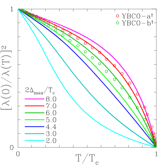
Figure 8: The penetration depth, $[\lambda(0)/\lambda(T)]^{2}$, for different values of $2\mit\Delta_{\rm max}/T_{c}$. From top to bottom the values are: 8, 7, 6, 5, 4.4, 3 and 2. The data points are from microwave experiments.[12]

Figure 9: Model of YBCO Fermi surfaces for chains (long dashed curve) and planes (closed short dashed curve) in the first Brillouin zone. The $(\pi,\pi)$ point is at the center of the figure. For the chains the parameters $\{t_{\alpha},\epsilon_{\alpha},B_{\alpha},\mu_{\alpha}\}$ in Eq. 22 are $\{-50,-0.9,0,1.2\}$ and for the planes they are $\{100,0,0.45,0.51\}$.

(a)		(c)		(e)
	=		+
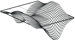
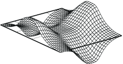
(b)		(d)		(f)
	=		+

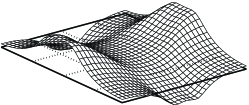
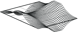
Figure 10: The order parameter in the first Brilliouin zone for (a) the plane layers and (b) the chain layers. Beside are the projections of the $d$ components, (c) and (d), and the $s$ components, (e) and (f). The vertical scale in all frames is the same. Note that the relative phase of the $d$-components in the two layers are the same while that of the $s$-components are opposite; this is caused by the interlayer interaction, $V_{{\bf k},{\bf q},12}$, being negative (ie, repulsive).

(a)	(c)	(e)
(b)	(d)	(f)

Figure 11: The Fermi surface (dashed curves) and gap nodes (solid curves) for a CuO₂ plane layer (top frames) and a CuO chain layer (bottom frames) for three different interlayer interaction strengths (left, middle and right frames). As the strength of the interlayer interaction, $g_{12}$, is increased (left to right frames) the proportion of the $s$-component in both layers increases. If the interlayer interaction were further increased the gap nodes would leave the Brillouin zone altogether and the order parameter would become $s$-like. Note that the Fermi surface in the CuO₂ plane layer is tetragonal but that the gap node is orthorhombic.

(a)	(b)	(c)	(d)

Figure 12: Calculation of the zero temperature order parameters as a function of the interlayer interaction, $g_{12}$, for two fixed values of the interlayer interaction, $g_{11}$, (left and right pairs of frames) presented for the planes, (b) and (d), and chains, (a) and (c), separately. In all frames the solid curve is the $d$-wave component of the order parameter, the short dashed curve is the extended $s$-wave component and the long dashed curve is the isotropic $s$-wave component. In the left frames $g_{11}=26.2$ and for $g_{12}=10$, $T_{\rm c}=100K$. At $g_{12}=0$ the order parameter is zero in the chains and is pure $d$-wave in the planes. As the interlayer interaction is increased the order parameter becomes present in the chains and there is a mixing of $s$-wave components. In the right frames $g_{11}=9.18$ and for $g_{12}=20$, $T_{\rm c}=100K$. At $g_{12}=0$ the order parameter is zero in both the chains and the planes. As the interlayer interaction is increased the order parameter becomes present in both the chains and planes and there is a mixing of $s$-wave components with the isotropic $s$-wave component eventually becoming dominant. The feature at $g_{12}\sim 25$ occurs when the gap node leaves the Brillouin zone. As discussed in the text there is a $g_{12}\leftrightarrow-g_{12}$ symmetry. Both $g_{11}$ and $g_{12}$ are in units of $t_{1}$; $g_{22}$, the coupling in the chains, is set equal to zero.

If one wants to remain within a model where there is no pairing interaction in the chains, one way to increase the value of the chain gap is to include off diagonal pairing in a two band bcs model. The bcs equations in this case are [18-19]

$$\mit\Delta_{{\bf k},1} = \frac{1}{\Omega}\sum_{{\bf q}}{\left(V_{{\bf k},{\bf q},11}\chi_{{\bf q},1}+V_{{\bf k},{\bf q},12}\chi_{{\bf q},2}\right)}$$

$$\mit\Delta_{{\bf k},2} = \frac{1}{\Omega}\sum_{{\bf q}}{\left(V_{{\bf k},{\bf q},12}\chi_{{\bf q},1}+V_{{\bf k},{\bf q},22}\chi_{{\bf q},2}\right)},$$ (20)

where the pairing susceptibility is:

$$\chi_{{\bf q},\alpha} \equiv \left<c_{{\bf q}\uparrow,\alpha}c_{-{\bf q}\downarrow,\alpha}\right>$$ (21)

$$= \frac{\mit\Delta_{{\bf q},\alpha}}{2E_{{\bf q},\alpha}}\tanh\left(\frac{E_{{\bf q},\alpha}}{2k_{\rm B}T}\right),$$

for the $\alpha$’th band with the brackets $\left<\cdot\right>$ indicating a thermal average of the pair annihilation operators. In calculations, we will assume $V_{22}$ to be zero but take $V_{12}=V_{21}$ finite. This is the term that couples the chains and planes and makes the chains have a gap. For the electron dispersions, we take a model with up to second neighbour hopping with:

$$\xi_{{\bf k},\alpha} = -2t_{\alpha}\left[(1+\epsilon_{\alpha})\cos(k_{x})+\cos(k_{y})\right.$$ (22)

$$-\left.2B_{\alpha}\cos(k_{x})\cos(k_{y})-(2-2B_{\alpha}-\mu_{\alpha})\right],$$

where the two new parameters not in equation (1) and (2) are the second neighbour hopping $B_{\alpha}$ and the orthorhombic distortion $\epsilon_{\alpha}$. As a model we take $\{t_{\alpha},\epsilon_{\alpha},B_{\alpha},\mu_{\alpha}\}$ to be $\{100,0,0.45,0.51\}$ for the planes and $\{-50,-0.9,0,1.2\}$ for the chains. The resulting Fermi surfaces for chains (long dashes) and planes (short dashes) are shown in Fig. 9.

To solve for the gaps of equations (Interband Pairing), we need to make some choices for the pairing potential $V_{{\bf k},{\bf k^{\prime}},\alpha\beta}$. In the previous section, we chose a separable form. Here we use a different alternative, which is based on the nearly antiferromagnetic Fermi liquid approach, and assume:

$$V_{{\bf k},{\bf q},\alpha\beta}=g_{\alpha\beta}\frac{-t}{1+\xi_{\circ}^{2}|{\bf k-q-Q}|^{2}},$$ (23)

which is proportional to the antiferromagnetic spin susceptibility with magnetic coherence length $\xi$ taken from Millis, Monien and Pines [21] and $t=100$meV sets the energy scale. In equation (23), $\bf Q$ is the commensurate wave vector $(\pi,\pi)$ and therefore the repulsive interaction (23) is peaked at $(\pi,\pi)$. This interaction leads directly to a $d_{x^{2}-y^{2}}$ gap in a single plane. If the coupling $g_{\alpha\beta}$ for $\alpha\not=\beta$ is different from zero superconductivity is induced in the chains and the gap no longer has pure $d_{x^{2}-y^{2}}$ symmetry in both chains and planes. It will be an admixture of:

$$\eta_{\bf k}^{(s_{\circ})} = 1$$

$$\eta_{\bf k}^{(s_{x^{2}+y^{2}})} = \cos(k_{x})+\cos(k_{y})$$

$$\eta_{\bf k}^{(d_{x^{2}-y^{2}})} = \cos(k_{x})-\cos(k_{y}).$$

In Fig. 10, we show results for a case $\{g_{11},g_{12},g_{22}\}=\{26.2,10,0\}$ with the critical temperature taken to be 100 K representative of the copper oxides. What is shown in frames (a) and (b) are the gaps as a function of momentum in the first Brillouin zone for the plane and chain, respectively. The projection on d-wave and s-wave manifold are also shown in (c) and (e) for the plane and (d) and (f) for the chain. We see that the orthorhombic chains can lead to a significant mixture of $s$ and $d$ components even for the plane case.

A useful representation of these gap results is to show the contours of gap zeros on the same plot as the Fermi surface. This is presented in the series of frames shown in Fig. 11. The top frames apply to the planes while the bottom frames apply to the chains. In all cases, (a), (c), (e) for the planes and (b), (d), (f) for the chains, the same Fermi surface (dashed curves) was used. By choice, the Fermi contour have tetragonal symmetry in the top figure while the chain Fermi surface is a quasi straight line along $k_{x}$ as is expected for chains along $y$ in configuration space. The pictures are for three different values of pairing potential. The first set of two frames (a) and (b) are for $\{g_{11},g_{12},g_{22}\}=\{29.9,5,0\}$, i.e. very little coupling between chains and planes (off diagonal $g_{12}$ small). In this case, the gap in the plane is nearly pure d-wave as is also the induced gap in the chains. As the coupling $g_{12}$ is increased to $\{g_{11},g_{12},g_{22}\}=\{26.2,10,0\}$ a significant s-wave component gets mixed into both solutions and the gap nodes move off the main diagonals of the Brillouin zone. (This is the solution that is plotted in Fig. 10). The gap nodes still cross the Fermi surfaces in both chains and planes. As the coupling is further increased to $\{g_{11},g_{12},g_{22}\}=\{9.18,20,0\}$, Fig. 11 (e) and (d), the gap nodes move far off the diagonal and for the chains they no longer cross the Fermi surface so that there is a finite minimum value of the gap on this sheet of the Fermi surface.

The amount of admixture of each of the three components in equation (Interband Pairing) are shown as a function of off diagonal $g_{12}$ in Fig. 12 for the last two cases, namely $g_{22}=26.2$ left frames and $g_{11}=9.18$ right frames. The amplitude of the gap component involved is given in meV. Frames (a) and (c) are for the chains while frames (b) and (d) are for the planes. In all cases, the solid curve is the $d_{x^{2}-y^{2}}$-component, short dashed the $s_{x^{2}+y^{2}}$-component and long dashed the $s_{\circ}$-component.

For the first choice of intralayer interaction (left frames), $g_{11}=26.2$, and there is no order parameter in the chains when there is no interlayer interaction (ie, $g_{12}=0$) and the order parameter in the planes is pure $d$-wave. As the interlayer interaction is increased from zero, $s$-wave components appear in the planes and all three components appear in the chains. This “$s+d$ mixing” is caused by the breaking of the tetragonal symmetry upon the introduction of the chains; there is no relative phase between the $s$- and $d$-wave components within either the planes or chains but there can be a relative phase between the order parameter in the planes and chains. In the range of $g_{12}$ explored here the $d$-wave component in the plane remains dominant but for sufficiently strong interlayer interaction the isotropic $s$-wave component eventually dominates [13] (ie, the gap nodes disappear). For interaction parameters $\{g_{11},g_{12},g_{22}\}=\{26.2,10,0\}$ the critical temperature is 100K and the maximum value of the gap in the Brillouin zone is 27.5meV in the planes and 8.0meV in the chains, while the maximum values on the Fermi surfaces are approximately 22meV and 7meV respectively. The ratio $2\mit\Delta_{\rm max}/T_{\rm c}$ is 6.4 in the planes and 1.9 in the chains.

For the second choice of intralayer interaction (right frames), $g_{11}=9.18$, there is no order parameter in either the chains or the planes when there is no interlayer interaction (ie, $g_{12}=0$). As the interlayer interaction is increased $d$-wave and then $s$-wave components of the order parameter appear in both the planes and chains. Again, there is no relative phase between the $s$- and $d$-wave components within either the planes or chains but there can be an overall relative phase between the order parameter in the planes and chains. At approximately $g_{12}=15$ the gap nodes no longer cross the Fermi surface in the chains; the feature at $g_{12}\sim 25$ coincides with the gap nodes leaving the Brillouin zone and isotropic $s$-wave becoming dominant. For interaction parameters $\{g_{11},g_{12},g_{22}\}=\{9.18,20,0\}$ the critical temperature is again 100K and the maximum value of the gap in the Brillouin zone is now 32.8meV in the planes and 20.1meV in the chains, while the maximum values on the Fermi surfaces are approximately 27meV and 17meV respectively. The ratio $2\mit\Delta_{\rm max}/T_{\rm c}$ is 7.6 in the planes and 4.7 in the chains.

Note that for $g_{12}>0$ all of the $s$-wave components of the order parameters in both the planes and chains have the same relative sign and the $d$-wave components have opposite signs, while for $g_{12}<0$ all of the relative signs are reversed but that the magnitudes of the components are insensitive to the sign of $g_{12}$.

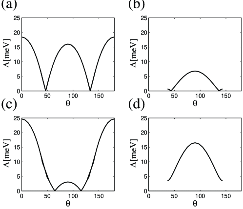
Figure 13: The magnitude of the gap on the Fermi surface as a function of angle for the four cases of Figs. 12. The angle $\theta$ is measured from the center or $(\pi,\pi)$ point of the Brillouin zone with the $y$-axis (ie, the vertical) corresponding to $\theta=0$. Frames (b) and (d) do not span all angles due to the Fermi surface not being closed in the chain layer. For the first choice of interaction parameters, $\{g_{11},g_{12},g_{22}\}=\{26.2,10,0\}$, the ratio $2\mit\Delta_{\rm max(FS)}/T_{\rm c}$, where $\mit\Delta_{\rm max(FS)}$ is the maximum value of the gap on the Fermi surface, is 4.3 and 1.6 for the planes and chain respectively; for the second, $\{g_{11},g_{12},g_{22}\}=\{9.18,20,0\}$, they are 5.7 and 3.8.

In Fig. 13 the magnitude of the gap is plotted as a function of angle, $\theta$, along the Fermi surface measured from the vertical. In frame (a) of Fig. 13 the local maxima of the gap on the Fermi surface are 16 and 18meV; in (b) they are 1 and 7meV, and in (c) they are 25 and 3meV. In (d) one can see that there are no gap nodes which cross the Fermi surface; the maximum and minimum value of the gap on the Fermi surface are 17 and 4meV respectively.

(a)	(b)

Figure 14: The magnetic penetration depth for the two sets of interaction parameters. Which show the magnetic penetration depth along (solid curve) and perpendicular (dashed curve) to the CuO chains. The dotted curve is $1-(T/T_{\rm c})^{2}$ and is shown for comparison. The chains, due to their Fermi surface, do not contribute appreciably to the penetration depth perpendicular to the chains (dashed curves). The ratio $(\lambda_{yy}/\lambda_{xx})^{2}$ is 1.37 for both sets of parameters since this is a normal state property.

In Fig. 14 we have plotted the magnetic penetration depth calculated with the lowest three harmonics (Interband Pairing) of the solutions of the bcs equations (Interband Pairing) for the two choices of interaction parameters. The solid curve is for the $y$-direction (along the chains) and the dashed curve is for the $x$-direction (perpendicular to the chains). The dotted curve is $1-(T/T_{\rm c})^{2}$ and is plotted for comparison. The ratio $\lambda_{yy}/\lambda_{xx}$ at zero temperature is 1.37 for both interaction parameter choices since the zero temperature penetration depth is a normal state property. The zero temperature penetration depth is largely governed by the bandwidth (ie, $4t_{\alpha}(2-\epsilon_{\alpha})$) – the larger the bandwidth the larger the zero temperature penetration depth.

As pointed out above, the curvature of the penetration depth curve, $\lambda_{ii}^{-2}(T)$, is largely governed by the ratio $2\mit\Delta_{\rm max}/T_{\rm c}$ and is a straight line for the $d$-wave bcs value of $4.4$. The presence of the chain layer and the interlayer interaction increases this ratio in the plane layer but it remains low in the chain layer due to the absence of an interaction in this layer. It is this lower value that makes $\lambda^{-2}_{yy}(T)$ (along the chains) have upward curvature (solid curves). Including pairing in the chains will push the solid curve towards the dashed one and make the initial low temperature slopes fall closer to each other.

Conclusions

In conclusion, the present data on single crystal untwinned YBCO at optimum doping suggest that the proximity effect incorporated into a single perpendicular tunnelling parameter $t_{\perp}$ cannot account for the observation. If interplane pairing is included the situation is greatly improved provided the off diagonal pairing is increased sufficiently to produce a gap on the chain which is of the same order of magnitude as that in the planes. Similar values of the gaps on the chains and planes can be taken as evidence that optimally doped YBCO is fairly three dimensional and that the coherence length in the $z$-direction may not be sufficiently short to allow spatial inhomogeneities to exist within a unit cell.

References

- [1] C.G. Olson et al., Science 245, 731 (1989).
- [2] Z.X. Shen et al., Phys. Rev. Lett. 70, 1553 (1993).
- [3] H. Ding, J.C. Campuzano et al., Phys. Rev. Lett. 50, 1333 (1994).
- [4] D.A. Wollman, D.J. Van Harlingen, W.C. Lee, D.M. Ginsberg and A.J. Leggett, Phys. Rev. Lett. 71, 2134 (1993).
- [5] C.C. Tsuei et al., Phys. Rev. Lett. 73, 593 (1994).
- [6] J.R. Kirtley, C.C. Tsuei, J.Z. Sun, C.C. Chi, Lock See Yu-Jahnes, A. Gupta, M. Rupp and M.B. Ketchen, Nature 373, 225(1995).
- [7] C.C. Tsuei et al., Science 271, 329 (1996).
- [8] Y. Zha, S.L. Cooper and D. Pines, preprint.
- [9] D.N. Basov, R. Liang, D.A. Bonn, W.N. Hardy, B. Dabrowski, M. Quijada, D.B. Tanner, J.P. Rice, D.M. Ginsberg and T. Timusk Phys. Rev. Lett. 74, 598 (1995).
- [10] D.A. Bonn, P. Dosanjh, R. Liang and W.N. Hardy, Phys. Rev. Lett. 68, 2390 (1992).
- [11] W.N. Hardy et al, Phys. Rev. Lett. 70, 3999 (1993).
- [12] D.A. Bonn, S. Kamal, K. Zhang, R. Liang, D.J. Baar, E. Kleit and W.N. Hardy, Phys. Rev. B 50, 4051 (1994).
- [13] A.I. Liechtenstein, I.I. Mazin and O.K. Anderson, Phys. Rev. Lett. 74, 2303 (1995).
- [14] H.L. Edwards, J.T. Markert, and A.L. de Lozanne, Phys. Rev. Lett. 73, 2967 (1992).
- [15] H.L. Edwards, D.J. Derro, A.L. Barr, J.T. Markert, and A.L. de Lozanne, Phys. Rev. Lett. 75, 1387 (1992).
- [16] W.A. Atkinson and J.P. Carbotte, Phys. Rev. B 51, 1161 (1995); Phys. Rev. B 51, 16371 (1995); .
- [17] W.A. Atkinson and J.P. Carbotte, Phys. Rev. B 52, 6894 (1995);
- [18] W.A. Atkinson and J.P. Carbotte, Phys. Rev. B 52, 10601 (1995);
- [19] C. O’Donovan and J.P. Carbotte, work in progress.
- [20] D.Z. Liu, K. Levin and J. Maly, Phys. Rev. B 51, 8680 (1995).
- [21] A.J. Millis, H. Monien and D. Pines, Phys. Rev. B 42, 167 (1990).